primer.ml.fine_tuning
Fine-tuning in practice: preparing data, forgetting old skills, merging models
Run: python -m primer.ml.fine_tuning
New to the notation? primer.notation explains every symbol used here
(Σ, ‖x‖, λ, subscripts, and so on) from zero.
This lesson builds on primer.ml.training_stages, which explains what
supervised fine-tuning (SFT), preference tuning and LoRA are. Here we deal
with what happens when you actually do it: deciding whether to fine-tune at
all, preparing the data, the old skills the model loses along the way, the
small dataset it memorises, and how two fine-tuned models can be merged into
one by plain arithmetic on their weights.
Level 1: The practitioner's guide
In one sentence. Fine-tuning in practice is the work around the training run: deciding with an evaluation set whether to train at all, preparing examples that teach what you mean, keeping the skills the model already had, stopping before it memorises your data, and sometimes combining two fine-tunes by arithmetic on their weights instead of training a third.
When you need it. You need this lesson when a fine-tune is on the table: a behaviour the best prompt cannot make consistent, or a long prompt sent so often that its tokens are most of the bill. The tell for the first is an eval score that stops improving however the prompt is reworded; the tell for the second is arithmetic. In this lesson's worked example, a 3,000-token prompt at \$2 per million tokens costs \$0.0060 per request, a tuned model that needs 300 tokens at \$4 per million costs \$0.0012, and a \$600 fine-tune pays for itself after 125,000 requests (25 days at 5,000 a day; the prices are illustrative). You don't need fine-tuning to add facts, which go stale the day they change and belong in retrieval, and you don't need it while a clearer instruction with two examples still moves the eval. Nothing in this lesson matters until the eval exists: it is the first box of the decision, before any model.
Your options. From the cheapest to the most committed:
| Option | What it does | What it guarantees | What it costs | Where it lives |
|---|---|---|---|---|
| The best prompt, scored on the eval | Instructions and examples in the prompt, measured on a frozen held-out set | A baseline every other option must beat; survives a base-model upgrade | Tokens on every call | Your prompt |
| Hosted supervised fine-tuning | Upload chat examples; the vendor applies the chat template, masks the user turns, trains and hosts | Consistent format and style without the long prompt | Curated examples, a training job, often a higher per-token price | The vendor's fine-tuning API |
| LoRA on an open model | Train a small adapter beside frozen weights on your examples | Learns the task with less forgetting of the base model's skills (Biderman et al., 2024) | A GPU, data, a serving stack; may learn a hard new domain less completely | Your training stack |
| Full fine-tune, with replay | Update every weight on your task mixed with a little general data | The largest change the model can make, and the old skills kept if you replay them | Multi-GPU training, the most forgetting when you don't replay, a copy of the model per variant | Your training stack |
| Merge existing fine-tunes | Add each fine-tune's task vector (its change from the base) to the base, no training | Two separable skills in one model at no extra inference cost | An eval on every task; fails when the two changes fight | Your weights, with a merging toolkit |
How to choose. Climb down only when the eval proves the rung above falls short.
- A format or a house style: a few dozen to a few hundred excellent examples, hosted or LoRA. Start with 50 to 100 and double only while a doubling still beats the eval's margin of error (section 2e).
- A behaviour that contradicts the base model ("always JSON" against "chat naturally", "be terse" against "explain"): expect the old behaviour to vanish wherever your data overrides it, and mix in general instruction-following data so the model stays an assistant (section 3c).
- A harder specialised skill: thousands of examples, and consider a full fine-tune with replay, since LoRA learns less on a demanding domain.
- Two skills trained separately, by different teams or on data that cannot be pooled: try a merge first, and check the cosine between the task vectors before you trust it (section 5b).
- Whatever you pick, the fine-tune ships only if it beats the prompt on the same held-out set by more than that set's margin of error, and a general eval sits beside the task eval.
What it costs. Money is the one-off cost of writing and checking data
plus the run, against a per-request saving that may be zero if the tuned
model is priced like the base one; the break-even rule in section 1 puts a
number on it. Every new base model repeats the one-off cost. Data is the
expensive part, and the eval is dearer than people expect: 100 held-out
examples measured at 80% mean "somewhere between 72% and 88%", and it takes
400 to halve that margin to ±3.9 points (this lesson's margin_of_error).
Labels cost accuracy too: with 10% of reference labels wrong, a perfect
model scores 90% and a 90% model scores 82%. Training itself is short.
In the lesson's toy the new task is learned in 5 steps and every step after
only erodes the general skill, and fine-tunes on small data run for a few
epochs, with the best checkpoint shipped rather than the last.
What breaks.
- The wrong chat template. Training succeeds, the loss falls, and the deployed model sees role markers it never learned. Use the exact template the base model was trained with, and the system prompt you will deploy.
- Training on the user's turns. Forget the loss mask and the model
learns to write questions. Hosted APIs mask for you;
render_chatshows which segments count. - A leaking eval. A training example that nearly copies a held-out one turns the eval into a memory test. Freeze the held-out set first and remove near-copies from training (Jaccard on word pairs, threshold 0.7 in the toy).
- Forgetting. Fine-tuning on one task takes the toy's general skill from 0.99 to 0.655, and a task that contradicts an earlier one takes the earlier one from 0.98 to 0.025. A lower learning rate only slows the slide; 10 replayed examples in 210 bring it back to 0.945.
- Memorising a small dataset. On 16 examples with 3 wrong labels, validation loss bottoms out at epoch 71 (0.319) and has quadrupled (1.277) by epoch 1,500. Checkpoint every epoch and ship the best.
- A merge that cancels. Task vectors with a clearly negative cosine (−0.25 in the toy) leave at least one skill at a coin flip whatever the scale. Retrain jointly, or use a conflict-resolving merge.
In the wild. Hosted fine-tuning APIs take chat-formatted examples and handle the template and the mask; OpenAI's model optimization guide lists supervised fine-tuning, DPO and reinforcement fine-tuning. For open models, Hugging Face TRL's SFTTrainer runs the supervised loop and PEFT supplies LoRA. Merging has its own toolkit: mergekit implements linear averaging, SLERP, task arithmetic, TIES, DARE and more. The evidence behind the advice is in the papers at the end of the lesson: LIMA's 1,000 curated examples, model soups for averaging fine-tunes of one task, task arithmetic for adding and subtracting them, TIES for resolving interference, elastic weight consolidation for when the old data is gone, and Biderman et al. on LoRA learning less and forgetting less.
Go deeper. Level 2 puts every claim above on a 97-weight model you can train in a fraction of a second: the break-even formula, the chat mask, Jaccard deduplication, the margin of error and the label-noise ceiling, forgetting measured as distance from the base, the overfitting curve with early stopping, and task vectors merged at every scale. If you only needed to decide whether and how to fine-tune, you are done.
Level 2: How it works, from scratch
Picture a skilled cook who joins your restaurant. They already know how to cook (that is the pretrained model). You want them to cook your menu, your way. You can hand them a note with every order (a prompt), give them the recipe binder to look things up in (retrieval, RAG), or send them on a course about your kitchen (fine-tuning). The course is the only option that changes the cook, and it comes with the risks every teacher knows: the lessons can be badly written, the cook can cram the practice exam instead of learning, and a month of drilling one cuisine can make them rusty at everything else.
Everything below is one of those risks, measured on a model small enough to train in a fraction of a second.
1. Should you fine-tune at all?
Everyday picture. Giving the cook a note with every order costs a little each time. The course costs a lot once, and it has to be repeated whenever you hire a new cook (switch to a newer base model). The course pays off only when the notes would otherwise be long, sent millions of times, or simply not enough to make the cook consistent.
Tiny worked example. A support bot sends a 3,000-token prompt full of instructions and examples on every request. A fine-tuned model has learned that behaviour and needs only 300 tokens of prompt. Take these illustrative prices (real ones vary by provider and change often): \$2 per million input tokens for the general model, \$4 per million for the tuned one, because hosting a custom model usually costs more per token.
| Tokens per request | Price per million | Cost per request | |
|---|---|---|---|
| prompted | 3,000 | \$2 | 3,000 × 2 / 1,000,000 = \$0.0060 |
| fine-tuned | 300 | \$4 | 300 × 4 / 1,000,000 = \$0.0012 |
Each request saves \$0.0048. Writing and checking 1,000 training examples plus the training run costs, say, \$600 once. After 600 / 0.0048 = 125,000 requests the course has paid for itself: 25 days at 5,000 requests a day.
flowchart TD
  E[Build the eval set first] --> P[Best prompt you can write]
  P --> M1{Good enough<br/>on the eval?}
  M1 -->|yes| SHIP[Ship the prompt]
  M1 -->|"no: missing facts"| R[Add retrieval, RAG]
  R --> M2{Good enough<br/>on the eval?}
  M2 -->|yes| SHIP
  M2 -->|"no: wrong behaviour, format or style"| FT[Fine-tune, often with LoRA]
  FT --> M3{Beats the prompt<br/>on the SAME eval?}
  M3 -->|yes, and pays off| SHIPFT[Ship the fine-tune]
  M3 -->|no| P
Reading it: start at the top, and notice that the first box is not a
model at all: it is the evaluation set, the fixed exam every option is
scored on. Each rung is cheaper and faster to change than the one below it,
so you climb down only when the eval proves the rung above falls short.
Missing knowledge goes to retrieval, because fine-tuning is a poor way to
add facts; wrong behaviour that no prompt can pin down goes to fine-tuning.
The last diamond matters most: a fine-tune ships only if it beats the prompt
on the same eval. primer.ml.training_stages has the same decision as a
flowchart of approaches; this one adds the measurement at every step.
Level 3: the formula and its symbols
$$ N^\star = \frac{C_{\text{once}}}{c_{\text{prompt}} - c_{\text{tuned}}}, \qquad c = \frac{t \cdot p}{10^6} $$
Symbols
| Symbol | Meaning here | In the example |
|---|---|---|
| $N^\star$ | "N-star": the break-even number of requests | 125,000 |
| $C_{\text{once}}$ | one-off cost: writing and checking data, the training run | \$600 |
| $c$ | cost of one request | |
| $c_{\text{prompt}}, c_{\text{tuned}}$ | cost of one request with the long prompt, and with the fine-tuned model | \$0.0060, \$0.0012 |
| $t$ | input tokens sent per request | 3,000 and 300 |
| $p$ | price in dollars per million input tokens | \$2 and \$4 |
| $10^6$ | one million: prices are quoted per million tokens |
In words: "divide what the course costs once by what it saves on each request; that is how many requests it takes to earn the cost back."
With the numbers: $c_{\text{prompt}}$ = 3,000 × 2 / 10⁶ = 0.006, $c_{\text{tuned}}$ = 300 × 4 / 10⁶ = 0.0012, so $N^\star$ = 600 / 0.0048 = 125,000.
Level 3: in Python
In Python:
# c = t·p / 1,000,000 for each option
c_prompt = 3000 * 2.0 / 1_000_000
c_tuned = 300 * 4.0 / 1_000_000
c_prompt, c_tuned  # → (0.006, 0.0012)
C_once = 600
# N* = C_once / (c_prompt − c_tuned)
N_star = C_once / (c_prompt - c_tuned)
round(N_star)  # → 125000
# days to break even at 5,000 requests a day
round(N_star / 5000, 1)  # → 25.0
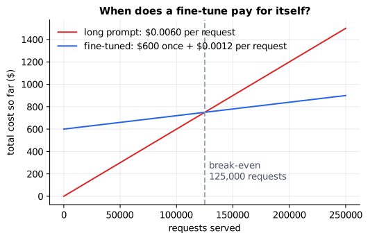
Reading it: the x-axis counts requests served and the y-axis is the total money spent so far. The prompted line starts at zero but climbs steeply, because every request pays for 3,000 tokens. The fine-tuned line starts at \$600 (the one-off cost) and climbs slowly. Left of the dashed line, prompting is cheaper; right of it, the fine-tune is. If the tuned model cost as much per request as the prompt, the two lines would never cross, and the only reason left to fine-tune would be quality.
In code: per_request_cost prices one request and
break_even_requests returns $N^\star$, or infinity when the tuned model
saves nothing per request.
Why it matters in practice. Three costs hide outside this formula.
Every new base model means repeating the fine-tune, so $C_{\text{once}}$
recurs. Facts learned by fine-tuning go stale and are hard to update, which
is why knowledge belongs in retrieval (primer.agents.rag). And the
engineering time to build an eval is spent whichever way you go, which is
why it comes first.
2. Preparing the data
Everyday picture. Before the course, someone writes the course book. Every recipe must be written in the same layout, no recipe may appear five times, some recipes are locked in a drawer for the final exam before the cook ever sees the book, and the recipes must actually be right. Most fine-tuning failures are course-book failures.
flowchart LR
  RAW[Raw examples<br/>logs, experts, drafts] --> FMT[Format as chat<br/>messages]
  FMT --> VAL[Validate<br/>roles, empty turns]
  VAL --> DD[Deduplicate<br/>near-copies]
  DD --> SPLIT[Set aside the<br/>held-out set, frozen]
  SPLIT --> LEAK[Drop training examples<br/>that copy held-out ones]
  LEAK --> AUDIT[Audit a sample<br/>of the labels]
  AUDIT --> TRAIN[Training set]
  SPLIT --> EVAL[Held-out set]
Reading it: raw examples enter on the left and pass through five filters. The branch at "Set aside the held-out set" is the important one: the held-out examples leave the pipeline before anything is trained or tuned, and the step after it removes any training example that nearly copies one of them. The subsections below build each box.
2a. Formatting chat examples
Everyday picture. A play script: every line starts with who speaks it. The model learns the play by reading scripts, and it is graded only on the lines of the character it will play, the assistant.
Tiny worked example. One example as a list of role-tagged messages:
| Turn | Role | Content | Trained on? |
|---|---|---|---|
| 1 | system | Be brief. | no |
| 2 | user | Capital of France? | no |
| 3 | assistant | Paris. | yes |
Rendered into text, it becomes
<|system|>Be brief.<|end|><|user|>Capital of France?<|end|><|assistant|>Paris.<|end|>,
and only the last segment counts towards the loss.
flowchart LR
  S["system: Be brief."] --> U["user: Capital of France?"] --> A["assistant: Paris."]
  S -.->|"context only, no loss"| L[Loss]
  U -.->|"context only, no loss"| L
  A ==>|"every token scored"| L
Reading it: the solid arrows are the order the model reads the turns.
The dotted arrows carry no training signal: the system and user turns are
context the model conditions on. Only the thick arrow feeds the loss, so the
model learns to answer, not to write questions. This is the loss mask from
primer.ml.training_stages, section 2.
The rules that matter. Use the exact chat template the base model was trained with; the role markers above are illustrative, and each model family has its own. Train with the same system prompt you will deploy with. Reject examples whose last turn is not the assistant's (nothing to learn), whose turns are empty, or whose roles are unknown.
In code: chat_example builds the message list, render_chat flattens
it into (segment, trained?) pairs, and validate_chat lists every problem
with an example.
Why it matters in practice. A template mismatch is silent: training succeeds, the loss falls, and the deployed model sees markers it never learned, so it behaves like the base model or worse.
2b. Deduplication
Everyday picture. A flashcard deck with the same card in it five times. You study that card five times as often, and you start answering every question with it.
Tiny worked example. Compare questions by their word pairs (two neighbouring words; a window of k words is called a shingle), after lowercasing and dropping punctuation:
| Text | Word pairs |
|---|---|
| "How do I reset my password?" | how do, do i, i reset, reset my, my password |
| "how do I reset my password, please" | the same 5, plus password please |
| "How do I change my email?" | how do, do i, i change, change my, my email |
The first two share 5 of the 6 distinct pairs between them: a near-duplicate. The first and third share 2 of 8: different questions.
Level 3: the formula and its symbols
$$ J(A, B) = \frac{|A \cap B|}{|A \cup B|} $$
Symbols
| Symbol | Meaning here | In the example |
|---|---|---|
| $A, B$ | the sets of word pairs of two texts | 5 pairs and 6 pairs |
| $\cap$ | intersection: pairs in both sets | 5 shared pairs |
| $\cup$ | union: pairs in either set, each counted once | 6 distinct pairs |
| $\lvert \cdot \rvert$ | the number of items in a set | |
| $J(A, B)$ | Jaccard similarity, from 0 (nothing shared) to 1 (identical) | 0.83 |
In words: "count the pairs the two texts share, and divide by the number of distinct pairs they have between them."
With the numbers: J = 5 / 6 = 0.83 for the two password questions and 2 / 8 = 0.25 for password against email. A threshold of 0.7 keeps the first password question, drops its rewording, and keeps the email question.
Level 3: in Python
In Python:
def pairs(text):
    words = text.lower().replace("?", "").replace(",", "").split()
    return {(a, b) for a, b in zip(words, words[1:])}
A = pairs("How do I reset my password?")
B = pairs("how do I reset my password, please")
C = pairs("How do I change my email?")
# |A ∩ B| and |A ∪ B|
len(A & B), len(A | B)  # → (5, 6)
# J(A, B)
round(len(A & B) / len(A | B), 2)  # → 0.83
# J(A, C)
len(A & C) / len(A | C)  # → 0.25
flowchart LR
  T[Next example] --> CMP{Jaccard with any<br/>kept example ≥ 0.7?}
  CMP -->|yes| DROP[Drop it:<br/>a near-copy]
  CMP -->|no| KEEP[Keep it]
  KEEP --> T
  DROP --> T
Reading it: examples arrive one at a time and are compared against everything already kept. A match above the threshold is dropped; anything else joins the kept list. The first copy of each group survives, so the order of the data decides which wording you keep.
In code: normalize lowercases and strips punctuation, shingles
collects the word pairs, jaccard scores two texts and deduplicate
returns the indices worth keeping. Comparing every pair is fine for
thousands of examples; at web scale, MinHash estimates the same Jaccard
without comparing every pair.
Why it matters in practice. Duplicates overweight a few examples, so the model parrots them. Worse, a near-copy of an eval question in the training set lets the model recite the answer, and the eval score becomes a memory test. Lee et al. found training sets with thousands of near-duplicates, and removing them made models memorise less.
2c. The held-out set comes first
Everyday picture. A good teacher writes the final exam before teaching the course and locks it in a drawer. If the exam were written afterwards, it would drift towards what the class happened to practise.
Tiny worked example. Fifty support questions are deduplicated, shuffled with a fixed seed, and 10 (20%) go in the drawer. Only then are the other 40 used, and any of the 40 that nearly copies one of the 10 is removed. Every later choice (prompt wording, learning rate, which checkpoint to ship) is scored on those 10. But how much can 10, or even 100, questions tell you?
Level 3: the formula and its symbols
$$ \text{margin} = z \sqrt{\frac{a\,(1 - a)}{n}} $$
Symbols
| Symbol | Meaning here | In the example |
|---|---|---|
| $a$ | the accuracy measured on the held-out set | 0.8 |
| $n$ | the number of held-out examples | 100 |
| $\sqrt{a(1-a)/n}$ | the standard error: how much the measured accuracy would wobble if you drew a different held-out set of the same size | 0.04 |
| $z$ | how many standard errors to allow; 1.96 covers 95% of the wobble | 1.96 |
| margin | the true accuracy is probably within ± this of the measured one | 0.078 |
In words: "the measured accuracy is uncertain by about two standard errors, and the standard error shrinks with the square root of the number of examples."
With the numbers: with 100 examples at 80%, the margin is 1.96 × √(0.8 × 0.2 / 100) = 1.96 × 0.04 = 0.078, so "80%" means "somewhere from about 72% to 88%". A fine-tune that scores 83% has not been shown to beat a prompt that scores 80%. With 400 examples the margin halves to 0.039.
Level 3: in Python
In Python:
import math
a, n, z = 0.8, 100, 1.96
# the standard error sqrt(a(1 − a)/n)
round(math.sqrt(a * (1 - a) / n), 4)  # → 0.04
# the 95% margin
round(z * math.sqrt(a * (1 - a) / n), 4)  # → 0.0784
# four times as many examples halves it
round(z * math.sqrt(a * (1 - a) / 400), 4)  # → 0.0392
flowchart LR
  ALL[All examples,<br/>deduplicated] --> SH[Shuffle with<br/>a fixed seed]
  SH --> EV[20% held out<br/>frozen, never trained on]
  SH --> TR[80% training]
  EV --> CHK{Training example<br/>near-copies one?}
  TR --> CHK
  CHK -->|yes| X[Remove from training]
  CHK -->|no| OK[Keep for training]
Reading it: the fixed seed makes the split repeatable, so everyone on a team scores against the same held-out set. The held-out branch is frozen the moment it is made. Both branches then meet in the leak check, which only ever removes examples from the training side.
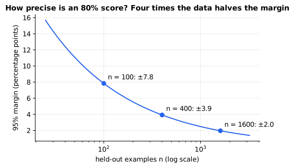
Reading it: the x-axis is the number of held-out examples (log scale) and the y-axis is the ± margin, in percentage points, around a measured 80%. The marked points show the square-root law: 100 examples give ±7.8 points, 400 give ±3.9 and 1,600 give ±2.0. Each halving of the margin costs four times the examples, which is why held-out sets of a few hundred are common and a few dozen can only detect big differences.
In code: split_before_training deduplicates, shuffles with a seed,
freezes the held-out set and removes leaks with remove_leaks;
margin_of_error gives the ± for any accuracy and size.
Why it matters in practice. Every time you look at held-out scores and
change something, the held-out set leaks a little into your decisions. A
held-out set built first and used sparingly is the only honest measure of
whether the fine-tune helped. See primer.ml.regularization for train,
validation and test splits, and primer.agents.evals for building evals.
2d. Label quality
Everyday picture. An answer key with typos. A student who gets every question right is marked wrong wherever the key is wrong, and a student who makes the same mistake as the key is marked right.
Tiny worked example. A model is truly right 90% of the time, and 10% of the reference labels are wrong. It scores a point when it is right on a right label (0.9 × 0.9 = 0.81), or when it is wrong on a wrong label and the two mistakes cancel (0.1 × 0.1 = 0.01). The eval reports 82%, not 90%.
Level 3: the formula and its symbols
$$ a_{\text{measured}} = a\,(1 - \varepsilon) + (1 - a)\,\varepsilon $$
Symbols
| Symbol | Meaning here | In the example |
|---|---|---|
| $a$ | the model's true accuracy | 0.9 |
| $\varepsilon$ | epsilon: the share of reference labels that are wrong | 0.1 |
| $a(1-\varepsilon)$ | right answer, right label | 0.81 |
| $(1-a)\varepsilon$ | wrong answer on a wrong label (yes/no labels only, so the two errors agree) | 0.01 |
| $a_{\text{measured}}$ | what the eval reports | 0.82 |
In words: "the eval gives credit for being right on a correct label, and by accident for being wrong on a wrong one."
With the numbers: 0.9 × 0.9 + 0.1 × 0.1 = 0.82. A perfect model ($a = 1$) scores only 1 − ε = 0.9: noisy labels put a ceiling on what the eval can show.
Level 3: in Python
In Python:
a, eps = 0.9, 0.1
# right on a right label, plus wrong on a wrong label
round(a * (1 - eps) + (1 - a) * eps, 2)  # → 0.82
# even a perfect model scores only 1 − ε
round(1.0 * (1 - eps), 2)  # → 0.9
# two labelers, five items: how often do they agree?
labeler_1 = ["yes", "no", "yes", "yes", "no"]
labeler_2 = ["yes", "no", "no", "yes", "no"]
sum(p == q for p, q in zip(labeler_1, labeler_2)) / len(labeler_1)  # → 0.8
flowchart TD
  X[One eval item] --> R{Model right?}
  R -->|"yes, 0.9"| LR{Label right?}
  R -->|"no, 0.1"| LW{Label right?}
  LR -->|"yes, 0.9"| P1["scored right: 0.81"]
  LR -->|"no, 0.1"| P2["scored wrong: 0.09"]
  LW -->|"yes, 0.9"| P3["scored wrong: 0.09"]
  LW -->|"no, 0.1"| P4["scored right: 0.01"]
Reading it: each item takes two coin flips: is the model right, and is the label right? Multiply along a path to get its share. Two paths are scored as right, 0.81 and 0.01, which add up to the 0.82 the eval reports. The 0.09 on the second path is a correct answer marked wrong by a bad label.
How to check label quality. Have two people label the same sample independently and measure how often they agree. Above, they agree on 4 of 5 items, 80%: one item in five is ambiguous or mislabelled, and your eval can't resolve differences smaller than that noise. Read every disagreement; they are usually unclear instructions, not careless labelers.
In code: measured_accuracy applies the formula and label_agreement
compares two labelers.
Why it matters in practice. Bad training labels teach the model the mistakes (section 4 shows a small model memorising three of them). Bad eval labels hide real improvements. Zhou et al. (LIMA) fine-tuned a large model on just 1,000 carefully chosen examples and got a strong assistant: quality of examples beats quantity.
2e. How many examples?
Everyday picture. Teaching a house style is not teaching a language. A new cook learns how you plate a dish from a few dozen good examples; they don't need ten thousand.
Tiny worked example. Fine-tuning teaches a behaviour the base model can almost do already, so the useful sizes are small: a few dozen examples to show a format, hundreds for a consistent style or a narrow task, thousands for a harder specialised skill. Section 4 fine-tunes on 16 examples and shows the other side: with so few, the model soon memorises them, noise included.
flowchart LR
  S[Start with 50 to 100<br/>high-quality examples] --> T[Fine-tune]
  T --> E[Score on the<br/>held-out set]
  E --> Q{Gained more than<br/>the margin of error?}
  Q -->|yes| D[Double the data] --> T
  Q -->|no| STOP[Stop adding data:<br/>fix quality or approach]
Reading it: the loop grows the dataset only while each doubling still buys a real improvement, meaning one larger than the held-out margin from section 2c. When a doubling stops paying, more of the same data won't help; the fix is better examples or a different approach.
Why it matters in practice. Labelled data is the expensive part of fine-tuning. Doubling until the gains flatten spends it where it helps, and the held-out set tells you when to stop.
3. Catastrophic forgetting
Everyday picture. Someone who learned to drive in Britain, keeping left, moves to the United States and practises keeping right every day for a month. The new habit wins, and on a trip home they drift to the wrong side of the road. Nobody told them to forget the old rule; the new practice simply rewrote the reflex both rules use. Neural networks do this to an extreme: train on a new task alone and an old one can vanish. This is catastrophic forgetting.
The model we'll fine-tune. To watch it happen, we need a model small enough to train instantly. Each example is four numbers, and the answer is yes or no:
| Task | Inputs it uses | Rule | Plays the role of |
|---|---|---|---|
| general | all four, anywhere in [−3, 3] | yes when x₁ + x₃ > 0 | the base model's pretraining |
| A | x₁ in [−3, −1], x₂ in [−2, 2] | yes when x₂ > 0 | keep left in Britain |
| B | x₁ in [1, 3], x₂ in [−2, 2] | yes when x₂ < 0 | keep right in the US |
| C | x₃, x₄ in [−2, 2] | yes when x₃ + x₄ > 0 | an unrelated skill |
A and B read the same two inputs and apply opposite rules in different regions, so one model can learn both, but only by paying attention to the region. C reads inputs that A and B never touch.
flowchart LR
  X["4 inputs<br/>x1 x2 x3 x4"] --> H["16 hidden units<br/>tanh"]
  H --> O["1 output<br/>probability of yes"]
  TH["θ: all 97 weights<br/>in one vector"] -.-> H
  TH -.-> O
Reading it: four numbers go in, 16 hidden units each mix all of them,
and one output unit turns the hidden units into a probability. Every weight
(64 in the first layer, 16 hidden biases, 16 output weights and one output
bias) sits in a single vector θ of 97 numbers. Every task flows through the
same hidden units, which is exactly why one task's training can damage
another. primer.ml.neural_net builds this kind of network from scratch.
The base model is this network trained on the general task (99% accuracy on held-out examples). Every fine-tune below starts from it and runs plain gradient descent on 200 examples.
In code: TinyNet holds θ and computes predictions, loss and
TinyNet.gradient; make_task draws examples for each of the TASKS;
base_model pretrains the base and fine_tune trains a copy, leaving the
starting model untouched.
3a. The general skill fades while you teach a new one
Everyday picture. A month of drilling one cuisine makes the cook a little rusty at everything else, and a second month of drilling it makes them rustier still, even though they had mastered the cuisine in the first week.
Tiny worked example. Fine-tune the base on task A (learning rate 0.5) and check both skills on held-out examples:
| After step | Accuracy on A | General skill | Distance from base |
|---|---|---|---|
| 0 (the base) | 0.53 | 0.99 | 0 |
| 5 | 0.975 | 0.825 | 2.60 |
| 10 | 0.995 | 0.79 | 2.83 |
| 300 | 0.98 | 0.655 | 5.19 |
Task A is learned in 5 steps. The next 295 steps teach nothing new about A but keep eroding the general skill, from 0.825 to 0.655. The last column explains why: the weights keep travelling away from the base.
Level 3: the formula and its symbols
$$ d_t = \lVert \theta_t - \theta_{\text{base}} \rVert = \sqrt{\sum_{i=1}^{P} \left(\theta_{t,i} - \theta_{\text{base},i}\right)^2} $$
Symbols
| Symbol | Meaning here | In the example |
|---|---|---|
| $\theta_{\text{base}}$ | theta: every weight of the base model, as one vector | 97 numbers |
| $\theta_t$ | every weight after $t$ fine-tuning steps | |
| $P$ | the number of weights | 97 (3 in the hand example) |
| $i$ | a counter over the weights | 1 … P |
| $\theta_{t,i}$ | the $i$-th weight after $t$ steps | |
| $\lVert v \rVert$ | the length of vector $v$: square each entry, add, take the square root | |
| $d_t$ | how far fine-tuning has moved the model | 5.19 after 300 steps |
In words: "the distance travelled is the length of the change in the weights: square every weight's change, add them up, take the square root."
With the numbers: for a three-weight model moving from (1, 0, 2) to (1.5, −1, 2), the changes are (0.5, −1, 0), and d = √(0.25 + 1 + 0) = √1.25 = 1.118.
Level 3: in Python
In Python:
import math
theta_base = [1.0, 0.0, 2.0]
theta_t = [1.5, -1.0, 2.0]
# each weight's change
[t - b for t, b in zip(theta_t, theta_base)]  # → [0.5, -1.0, 0.0]
# ‖θ_t − θ_base‖
round(math.sqrt(sum((t - b) ** 2 for t, b in zip(theta_t, theta_base))), 3)  # → 1.118
flowchart LR
  DA[Task A examples] -->|gradient| W["Shared weights θ"]
  W --> SA[Answers on task A]
  W --> SG[Answers on the<br/>general skill]
  SG -.->|"no examples,<br/>no gradient"| W
Reading it: the gradient from task A's examples moves the shared weights, and both skills read those same weights. The dotted arrow is what is missing: the general skill has no examples in this training run, so nothing pushes back when a change that helps A hurts it. Forgetting is not an event; it is the absence of a counterweight.
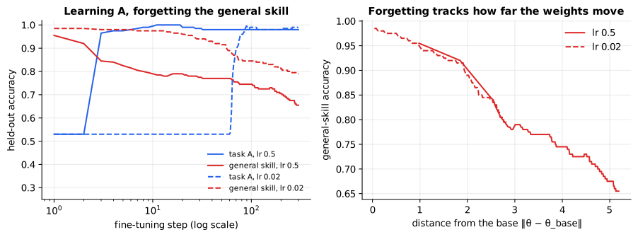
Reading it: on the left, the x-axis is the training step (log scale). Blue lines are accuracy on task A, red lines the general skill; solid is learning rate 0.5, dashed is 0.02. With the big rate, A is learned within a few steps and the general skill then slides for the rest of the run. With the small rate, A is learned later (around step 70) and the general skill ends at 0.79 instead of 0.655, with A just as good. On the right, every step of both runs is plotted as distance from the base against the general skill: the points fall along one downward curve. Forgetting tracks how far the weights move.
Mitigations that shorten the trip. Three knobs limit the distance, and the toy measures two of them:
- Fewer steps. Stop once the held-out score on the new task stops improving. Here, stopping at step 10 keeps the general skill at 0.79 instead of 0.655, with A at 0.995.
- A lower learning rate. Smaller steps travel less far for the same result: 0.79 instead of 0.655 after 300 steps.
- A smaller update. LoRA (
primer.ml.training_stages, section 4) freezes the base weights and allows only a low-rank change. Biderman et al. measured this on real language models and summed it up in their title: LoRA learns less and forgets less.
In code: general_skill_run fine-tunes on A and records, after every
step, accuracy on A, the general skill and the distance from the base.
Why it matters in practice. A fine-tuned assistant that has become worse at everything outside its narrow task is the most common fine-tuning disappointment. Always score the general skills you care about alongside the new task, and prefer the earliest checkpoint that has learned the task.
3b. A new task that contradicts an old one
Everyday picture. Back to the driver. Practising "keep right" does not merely add a skill; it pushes directly against "keep left", because both use the same reflex.
Tiny worked example. Take the model fine-tuned on A (98% on A), then fine-tune it on B alone for 300 steps:
| Second fine-tune | A before | A after | New task after |
|---|---|---|---|
| on B (contradicts A) | 0.98 | 0.025 | 1.00 |
| on C (separate inputs) | 0.98 | 0.97 | 0.98 |
After B, the model does not merely forget A; it answers A's questions backwards, because it learned "yes when x₂ < 0" everywhere. After C, A is barely touched: C's inputs never flowed through the weights A relies on most.
Level 3: the formula and its symbols
$$ F = \text{acc}_{\text{old}}^{\text{before}} - \text{acc}_{\text{old}}^{\text{after}} $$
Symbols
| Symbol | Meaning here | In the example |
|---|---|---|
| $\text{acc}_{\text{old}}^{\text{before}}$ | held-out accuracy on the old task before the new fine-tune | 0.98 |
| $\text{acc}_{\text{old}}^{\text{after}}$ | the same, after the new fine-tune | 0.025 |
| $F$ | forgetting: accuracy lost on the old task | 0.955 |
In words: "forgetting is how much accuracy the old task lost."
With the numbers: F = 0.98 − 0.025 = 0.955 after B, and 0.98 − 0.97 = 0.01 after C.
Level 3: in Python
In Python:
acc_before, acc_after_B, acc_after_C = 0.98, 0.025, 0.97
# F after the contradicting task B
round(acc_before - acc_after_B, 3)  # → 0.955
# F after task C, on separate inputs
round(acc_before - acc_after_C, 3)  # → 0.01
flowchart LR
  BASE[Base] -->|fine-tune on A| MA["Model knows A<br/>A: 0.98"]
  MA -->|fine-tune on B only| MB["Model knows B<br/>A: 0.025, B: 1.00"]
  MA -->|fine-tune on C only| MC["Model knows A and C<br/>A: 0.97, C: 0.98"]
Reading it: both second fine-tunes start from the same model. The only difference is which weights the new task needs: B needs the very ones A uses, in the opposite direction; C mostly needs others. How much a model forgets depends less on how long you train than on how much the new task overlaps and conflicts with the old one.
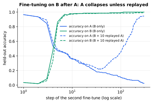
Reading it: the x-axis is the step of the second fine-tune (log scale), the y-axis held-out accuracy. Solid lines are plain fine-tuning on B: B (green) climbs to 1 while A (blue) falls to about half in the same few steps, and A keeps sliding towards zero for as long as training continues. Dashed lines add 10 replayed A examples (section 3c): A still dips at first (to about 0.2 around step 40), then climbs back to 0.945 while B reaches 0.99.
Does a lower learning rate help here? Only in the sense of slowing the slide. At learning rate 0.02, or stopping after 10 steps, B reaches 0.975 and A still drops to 0.355.
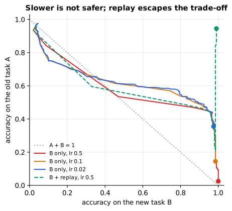
Reading it: each line traces one run: x is accuracy on B, y is accuracy on A, and each run starts at the top left (knows A, not B). The three learning rates (0.5, 0.1, 0.02) take very different numbers of steps but trace the same curve, close to the dotted line where A + B = 1: every point of B they gain costs about a point of A, and once B is learned, further steps slide A down the right edge towards zero. The replay run (dashed) follows the same curve at first, then climbs the right edge and ends in the top-right corner, knowing both. When the new data contradicts the old skill, slowing down can't help, because nothing in B's data says A still matters.
In code: sequential_run starts from the A fine-tune, trains on a new
task (optionally with replay), and records both accuracies at every step;
forgetting computes F.
Why it matters in practice. Real fine-tunes contradict the base model more often than you'd think: "always answer in JSON" contradicts "chat naturally"; "be terse" contradicts "explain in detail". Expect the old behaviour to vanish wherever your data overrides it, and test for it.
3c. Replay: keep practising the old skill
Everyday picture. A pianist learning a new piece plays one old piece at the start of every practice session. It costs a few minutes and keeps the old repertoire alive.
Tiny worked example. Add just 10 of task A's 200 training examples to B's 200: under 5% of the mix. The result: A 0.945, B 0.99 (up from A 0.025 without replay). Why can so few examples do so much? Look at the loss. Suppose that early in training the model already scores B well (loss 0.05 per example) but has started forgetting A (loss 3.0 on each replayed example):
Level 3: the formula and its symbols
$$ \mathcal{L}_{\text{mix}} = \frac{n_{\text{new}}\,\mathcal{L}_{\text{new}} + n_{\text{old}}\,\mathcal{L}_{\text{old}}}{n_{\text{new}} + n_{\text{old}}} $$
Symbols
| Symbol | Meaning here | In the example |
|---|---|---|
| $n_{\text{new}}$ | examples of the new task | 200 |
| $n_{\text{old}}$ | replayed examples of the old task | 10 |
| $\mathcal{L}_{\text{new}}$ | average loss on the new examples | 0.05 |
| $\mathcal{L}_{\text{old}}$ | average loss on the replayed examples | 3.0 |
| $\mathcal{L}_{\text{mix}}$ | the loss training actually minimises: the average over every example in the mix | 0.19 |
In words: "the loss on a mixed dataset is the average over all its examples, so each group counts in proportion to its size times its loss."
With the numbers: (200 × 0.05 + 10 × 3.0) / 210 = (10 + 30) / 210 = 0.19. The 10 replayed examples are under 5% of the data but contribute 0.143 of the 0.19: three quarters of the loss, and so most of the gradient. The old examples shout loudest exactly when they are being forgotten.
Level 3: in Python
In Python:
n_new, L_new = 200, 0.05
n_old, L_old = 10, 3.0
# the replayed share of the data
round(n_old / (n_new + n_old), 3)  # → 0.048
# each group's contribution to the average loss
round(n_new * L_new / 210, 3), round(n_old * L_old / 210, 3)  # → (0.048, 0.143)
# L_mix
round((n_new * L_new + n_old * L_old) / (n_new + n_old), 2)  # → 0.19
flowchart LR
  NB["New task B<br/>200 examples"] --> MIX[Shuffle together<br/>210 examples]
  OA["Old task A<br/>10 kept examples"] --> MIX
  MIX --> FT[Fine-tune]
  FT --> BOTH["Knows B: 0.99<br/>and A: 0.945"]
Reading it: the old task's small sample joins the new data before training, so every gradient step sees both. This supplies exactly the counterweight that was missing in section 3a's diagram: when a change that helps B starts hurting A, the replayed examples' loss rises and pushes back.
In code: replay_mix appends the old examples, mixed_loss is the
formula, and sequential_run with n_replay=10 runs the experiment.
Why it matters in practice. When fine-tuning a language model, mix some general instruction-following data into your task data, so the model keeps being a good assistant while it learns your task. When you can't replay (the old data is gone or private), methods such as elastic weight consolidation (Kirkpatrick et al.) instead penalise changes to the weights the old task relied on most.
4. Overfitting a small dataset
Everyday picture. A student with only 16 flashcards, three of which
have the wrong answer on the back. For a while, studying teaches the
pattern. Keep drilling and the student memorises every card word for word,
including the three wrong answers, and gets worse on new questions.
primer.ml.regularization builds this idea from scratch; here it is in a
fine-tune.
Tiny worked example. Fine-tune the base on only 16 examples of task A, 3 of them deliberately mislabelled, for 1,500 epochs. (With full-batch training, one step is one pass over the data, one epoch.)
| At the best epoch (71) | At the end (1,500 epochs) | |
|---|---|---|
| training loss | 0.373 | 0.005 |
| validation loss | 0.319 | 1.277 |
At the best epoch, training loss is higher than validation loss: the model is refusing to fit the three wrong labels, which is exactly right. By the end, training loss is nearly zero, so the wrong labels have been memorised, and validation loss has quadrupled.
Level 3: the formula and its symbols
$$ g(t) = \mathcal{L}_{\text{val}}(t) - \mathcal{L}_{\text{train}}(t) $$
Symbols
| Symbol | Meaning here | In the example |
|---|---|---|
| $t$ | the epoch | 71, then 1,500 |
| $\mathcal{L}_{\text{train}}(t)$ | average loss on the 16 training examples | 0.373, then 0.005 |
| $\mathcal{L}_{\text{val}}(t)$ | average loss on 200 held-out examples | 0.319, then 1.277 |
| $g(t)$ | the generalisation gap: how much worse the model does on data it hasn't seen | −0.054, then 1.272 |
In words: "the gap is held-out loss minus training loss; a gap that keeps growing means the model is memorising rather than learning."
With the numbers: 0.319 − 0.373 = −0.054 at epoch 71; 1.277 − 0.005 = 1.272 at the end.
Level 3: in Python
In Python:
L_train = {"best": 0.373, "end": 0.005}
L_val = {"best": 0.319, "end": 1.277}
# g = L_val − L_train at each point
{t: round(L_val[t] - L_train[t], 3) for t in L_val}  # → {'best': -0.054, 'end': 1.272}
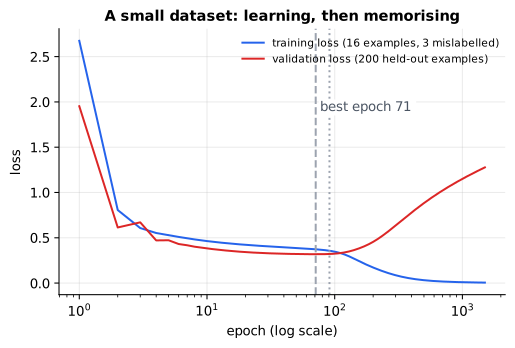
Reading it: the x-axis is the epoch (log scale), the y-axis the loss. Both curves fall at first while the model learns the real rule. At epoch 71 (the dashed line) validation loss bottoms out; after that the training curve keeps falling as the model memorises the three wrong labels, and the validation curve climbs. The dotted line is where early stopping with a patience of 20 epochs would end the run, keeping the weights from epoch 71.
flowchart LR
  EP[Train one epoch] --> SV[Save a checkpoint]
  SV --> SC[Score it on the<br/>held-out set]
  SC --> Q{Best so far?}
  Q -->|yes| MARK[Mark it best] --> EP
  Q -->|"no, patience used up"| SHIP[Ship the best checkpoint,<br/>not the last]
  Q -->|"no, patience left"| EP
Reading it: every epoch ends with a checkpoint and a held-out score. The loop keeps going while scores improve or patience remains, and when it stops, the checkpoint that ships is the marked best, not whatever the last epoch left behind.
In code: overfitting_run fine-tunes on the 16 examples and records
both losses every epoch; primer.ml.regularization.early_stopping replays
the validation curve and returns the best epoch and the stopping epoch.
Why it matters in practice. Fine-tuning datasets are small compared to pretraining, and big models memorise quickly, so fine-tunes typically run for only a few epochs. Save checkpoints, score each on the held-out set, and ship the best one.
5. Model merging
5a. Weight averaging and task arithmetic
Everyday picture. Two editors each take a copy of the same draft and make tracked changes: one fixes the grammar, the other tightens the argument. You can apply both sets of changes to the original. If instead you "average" the two edited copies, each change is applied at half strength: half the grammar fixed, half the argument tightened.
Tiny worked example. A three-weight base (1, 0, 2). One fine-tune moves it to (1.5, 0, 2); another to (1, −1, 2).
| Weights | Change from the base | |
|---|---|---|
| base | (1, 0, 2) | |
| fine-tune on A | (1.5, 0, 2) | τ_A = (0.5, 0, 0) |
| fine-tune on C | (1, −1, 2) | τ_C = (0, −1, 0) |
| base + τ_A + τ_C | (1.5, −1, 2) | both changes in full |
| average of the two fine-tunes | (1.25, −0.5, 2) | both changes at half strength |
The change a fine-tune made, θ_ft − θ_base, is its task vector. Adding task vectors to the base is task arithmetic.
Level 3: the formula and its symbols
$$ \tau_t = \theta_t - \theta_{\text{base}}, \qquad \theta_{\text{merged}} = \theta_{\text{base}} + \lambda \sum_{t=1}^{T} \tau_t $$
Symbols
| Symbol | Meaning here | In the example |
|---|---|---|
| $t$ | which task: a counter over the fine-tunes | A, C |
| $T$ | how many fine-tunes are merged | 2 |
| $\theta_t$ | all the weights of the model fine-tuned on task $t$ | (1.5, 0, 2) |
| $\theta_{\text{base}}$ | the weights they all started from | (1, 0, 2) |
| $\tau_t$ | tau: task $t$'s task vector, everything its fine-tune changed | (0.5, 0, 0) |
| $\sum_{t=1}^{T}$ | add up the task vectors | τ_A + τ_C = (0.5, −1, 0) |
| $\lambda$ | lambda: how strongly to apply the combined changes | 1 |
| $\theta_{\text{merged}}$ | the merged model's weights | (1.5, −1, 2) |
In words: "each task vector is what its fine-tune changed; add the changes up, scale them by λ, and apply them to the base."
With the numbers: θ_merged = (1, 0, 2) + 1 × (0.5, −1, 0) = (1.5, −1, 2). With λ = 1/2: (1, 0, 2) + 0.5 × (0.5, −1, 0) = (1.25, −0.5, 2), which is exactly the average of the two fine-tunes. Averaging T fine-tunes is task arithmetic with λ = 1/T.
Level 3: in Python
In Python:
theta_base = [1.0, 0.0, 2.0]
theta_A = [1.5, 0.0, 2.0]
theta_C = [1.0, -1.0, 2.0]
# τ_t = θ_t − θ_base
tau_A = [a - b for a, b in zip(theta_A, theta_base)]
tau_C = [c - b for c, b in zip(theta_C, theta_base)]
tau_A, tau_C  # → ([0.5, 0.0, 0.0], [0.0, -1.0, 0.0])
# θ_merged at λ = 1
[b + 1.0 * (a + c) for b, a, c in zip(theta_base, tau_A, tau_C)]  # → [1.5, -1.0, 2.0]
# λ = 1/2 ...
[b + 0.5 * (a + c) for b, a, c in zip(theta_base, tau_A, tau_C)]  # → [1.25, -0.5, 2.0]
# ... is the plain average of the two fine-tunes
[(a + c) / 2 for a, c in zip(theta_A, theta_C)]  # → [1.25, -0.5, 2.0]
flowchart LR
  B[Base θ] -->|fine-tune on A| FA[θ_A]
  B -->|fine-tune on C| FC[θ_C]
  FA --> TA["τ_A = θ_A − θ_base"]
  FC --> TC["τ_C = θ_C − θ_base"]
  TA --> SUM["λ × (τ_A + τ_C)"]
  TC --> SUM
  B --> ADD((+))
  SUM --> ADD
  ADD --> M[Merged model:<br/>no extra training]
Reading it: both fine-tunes start from the same base; that shared start is what makes their changes comparable. Subtracting the base turns each fine-tuned model into a task vector, the arrows are added and scaled, and the result is added back to the base. No data and no gradient steps are involved: merging is arithmetic on weights, and the merged model is the same size and speed as the base.
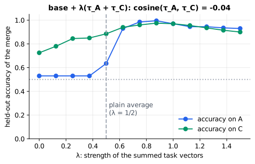
Reading it: the x-axis is λ and the y-axis held-out accuracy of the merged model on A (blue) and on C (green); the dotted line is 0.5, a coin flip. At λ = 1/2, which is plain averaging, each skill is diluted: 0.635 on A. Around λ = 1 the merged model does both tasks at 0.97, as well as either specialist on its own task. Push λ further and the changes overshoot. Their task vectors are nearly perpendicular (cosine −0.04), so adding one barely disturbs the other.
In code: task_vector subtracts the base, merge adds scaled task
vectors back, and merge_run merges two fine-tunes at several λ and scores
the result.
Why it matters in practice. Merging combines skills trained separately, by different teams or on data that can't be pooled, without any further training and at no extra inference cost. Averaging several fine-tunes of the same task ("model soups", Wortsman et al.) often beats the best single one. Task vectors can also be subtracted: Ilharco et al. negated a task vector learned from toxic text to make a model less toxic.
5b. Interference: when task vectors collide
Everyday picture. Two editors rewrote the same sentence in opposite directions, one making it warmer and one making it colder. Applying both sets of tracked changes gives a sentence neither intended.
Tiny worked example. Our three-weight changes again, plus a new one: τ_A = (0.5, 0, 0), τ_C = (0, −1, 0) and τ_B = (−0.4, 0, 0.3). τ_A and τ_C touch different weights: no conflict. τ_B pulls the first weight the other way from τ_A. The cosine measures how aligned two changes are:
Level 3: the formula and its symbols
$$ \cos(\tau_A, \tau_B) = \frac{\tau_A \cdot \tau_B}{\lVert \tau_A \rVert \, \lVert \tau_B \rVert} $$
Symbols
| Symbol | Meaning here | In the example |
|---|---|---|
| $\tau_A \cdot \tau_B$ | dot product: multiply matching entries, then add | 0.5 × (−0.4) = −0.2 |
| $\lVert \tau \rVert$ | a vector's length | 0.5 and 0.5 |
| $\cos$ | the cosine of the angle between the two changes: 1 same direction, 0 unrelated, −1 opposite | −0.8 |
In words: "multiply the changes weight by weight and add, then divide by both lengths, so only the direction counts."
With the numbers: τ_A · τ_B = 0.5 × (−0.4) + 0 + 0 = −0.2; ‖τ_A‖ = 0.5,
‖τ_B‖ = √(0.16 + 0.09) = 0.5; cos = −0.2 / 0.25 = −0.8: strongly
opposed. cos(τ_A, τ_C) = 0: independent. See primer.ml.embeddings.similarity
for the cosine from scratch.
Level 3: in Python
In Python:
import math
tau_A = [0.5, 0.0, 0.0]
tau_B = [-0.4, 0.0, 0.3]
tau_C = [0.0, -1.0, 0.0]
def cos(u, v):
    dot = sum(a * b for a, b in zip(u, v))
    return dot / (math.sqrt(sum(a * a for a in u)) * math.sqrt(sum(b * b for b in v)))
# opposed changes
round(cos(tau_A, tau_B), 2)  # → -0.8
# changes to different weights
cos(tau_A, tau_C)  # → 0.0
In the toy, the fine-tunes on A and on B (which reverses A's rule) have task vectors with cosine −0.25, against −0.04 for A and C. Each fine-tune learned its rule everywhere, not just in its own region, so the two vectors rewrite the same weights in opposite directions.
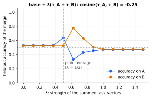
Reading it: the same axes as the previous figure, now merging A with B. No value of λ lifts both lines: wherever one task improves, the other sits near or below a coin flip, and from λ = 1 on both stay there, because the two changes cancel. A model can do both tasks (replay in section 3c got 0.945 and 0.99), but this merge can't reach it: that model needs to tell the regions apart, and neither fine-tune learned to.
flowchart TD
  TV[Task vectors from<br/>the same base] --> COS{Cosine between them}
  COS -->|"near 0: separate weights"| ADD[Add them:<br/>task arithmetic]
  COS -->|"clearly negative: conflict"| FIX{Can you retrain?}
  FIX -->|yes| JOINT[Train one model on<br/>both datasets, or replay]
  FIX -->|no| TIES["Resolve conflicts:<br/>trim small changes,<br/>agree on a sign per weight"]
  ADD --> EV[Score the merge on<br/>every task's held-out set]
  TIES --> EV
  JOINT --> EV
Reading it: a cheap check before merging is the cosine between task vectors. Near zero, the changes live in different weights and adding them usually works. Clearly negative, they fight: train on both datasets together if you can; if you can't, conflict-resolving merges such as TIES-merging (Yadav et al.) drop each task's smallest changes and, for each weight, keep only the changes that agree with the majority sign. Every path ends at the same place: score the merge on every task's held-out set.
In code: cosine measures the angle between two task vectors, and
merge_run reports it alongside the merged accuracies.
Why it matters in practice. Merges are free to try, which makes them tempting to trust. A merged model can quietly lose a skill both parents had, so it is evaluated like any new model. The cosine tells you in advance which merges to be nervous about.
In 20 seconds
- Decide with an eval: build a held-out set first; try prompting, then retrieval, and fine-tune only for behaviour a prompt can't pin down. It pays off after C / (c_prompt − c_tuned) requests.
- Data: use the model's chat template and train only on assistant turns; deduplicate (Jaccard on word shingles); freeze the held-out set before training and remove near-copies of it; audit labels, because wrong labels cap what the eval can show. Quality beats quantity.
- Forgetting: every weight is shared, so learning a new task erodes old ones, in proportion to how far the weights move and how much the tasks conflict. Fewer steps, a lower learning rate and LoRA shorten the trip; replaying a little old data is what keeps a contradicted skill.
- Overfitting: on small data, validation loss bottoms out early; ship the best checkpoint, not the last.
- Merging: a task vector is θ_ft − θ_base. Adding task vectors combines skills without training; averaging is λ = 1/T and dilutes them; vectors that point in opposite directions interfere.
Self-test questions
When is fine-tuning the wrong tool, and what should you try first? When the model lacks facts, or the facts change: retrieval supplies them and is easy to update. When a clearer prompt with a few examples fixes the behaviour: that is cheaper and survives a base-model upgrade. Fine-tuning earns its cost when behaviour stays inconsistent under the best prompt, or when a long prompt sent millions of times costs more than the fine-tune.
Why build the held-out set before training, and why check it against the training set? So that no choice (prompt, learning rate, checkpoint) is made by looking at it, and it stays an honest measure. A training example that nearly copies a held-out one lets the model recite the answer, turning the eval into a memory test; deduplicating across the split prevents it.
A held-out set has 100 examples and the fine-tune scores 83% against the prompt's 80%. Has it won? Not yet. At 80% on 100 examples the 95% margin is about ±7.8 points, so a 3-point difference is well inside the noise. You need a larger held-out set (400 examples halve the margin) or a bigger difference.
If 10% of the eval's labels are wrong, what is the best score a perfect model can get? 90%, because it is marked wrong on every mislabelled item. A 90%-accurate model would score 0.9 × 0.9 + 0.1 × 0.1 = 82%. Noisy labels shrink and blur the differences you are trying to measure.
What is catastrophic forgetting, and why does it happen? Training on a new task alone erodes, or wipes out, skills the model had. Every weight is shared between tasks, and only the new task's examples produce gradients, so nothing pushes back when a change that helps the new task hurts an old one. It grows with how far the weights move and with how much the new task conflicts with the old.
Lowering the learning rate did not stop task A being forgotten. Why not, and what works? Task B contradicts A on the same inputs, so any progress on B costs A; a lower rate only walks the same trade-off more slowly. Replay works: mixing even 5% of A's examples into B's data gives the model a reason to keep A, and those few examples carry most of the loss exactly when A is slipping.
Training loss keeps falling, but validation loss has risen since epoch 71. What is happening, and which checkpoint do you ship? The model has stopped learning the general rule and is memorising the training set, including its mislabelled examples. Ship the checkpoint from epoch 71, the best on the held-out set; early stopping automates exactly this.
What is a task vector, and why is averaging two fine-tunes the same as task arithmetic with λ = 1/2? A task vector is everything a fine-tune changed: θ_ft − θ_base. The average of two fine-tunes is (θ_base + τ_1 + θ_base + τ_2) / 2 = θ_base + ½(τ_1 + τ_2), which is task arithmetic with λ = 1/2, so each skill arrives at half strength.
When does merging fail, and how can you see it coming? When the task vectors change the same weights in opposite directions, so adding them cancels both skills. A clearly negative cosine between task vectors is the warning; the remedy is joint training or replay, or a conflict-resolving merge such as TIES, and a held-out check on every task either way.
The papers behind this lesson
- Ilharco et al., Editing Models with Task Arithmetic (2022): https://arxiv.org/abs/2212.04089. Defined task vectors as fine-tuned minus pretrained weights and showed that adding them combines skills, and negating them removes a behaviour. Annotated companion
- Wortsman et al., Model soups: averaging weights of multiple fine-tuned models improves accuracy without increasing inference time (2022): https://arxiv.org/abs/2203.05482. Showed that averaging the weights of several fine-tunes of one base often beats the best single fine-tune.
- Yadav et al., TIES-Merging: Resolving Interference When Merging Models (2023): https://arxiv.org/abs/2306.01708. Traced failed merges to small redundant changes and sign conflicts, and fixed both by trimming and electing a sign per weight.
- Kirkpatrick et al., Overcoming catastrophic forgetting in neural networks (2017): https://arxiv.org/abs/1612.00796. Introduced elastic weight consolidation, which slows learning on the weights most important to earlier tasks.
- Biderman et al., LoRA Learns Less and Forgets Less (2024): https://arxiv.org/abs/2405.09673. Measured on real language models that LoRA keeps more of the base model's abilities than full fine-tuning, at the price of learning the new task less completely.
- Zhou et al., LIMA: Less Is More for Alignment (2023): https://arxiv.org/abs/2305.11206. Fine-tuned a large base model on 1,000 carefully curated examples and got a strong assistant, evidence that example quality matters more than quantity. Annotated companion
- Lee et al., Deduplicating Training Data Makes Language Models Better (2021): https://arxiv.org/abs/2107.06499. Found widespread near-duplicates in standard datasets, including between training and test sets, and showed that removing them reduces memorisation.
Further reading
- Goodfellow et al., An Empirical Investigation of Catastrophic Forgetting in Gradient-Based Neural Networks (2013): https://arxiv.org/abs/1312.6211
- Hu et al., LoRA: Low-Rank Adaptation of Large Language Models (2021): https://arxiv.org/abs/2106.09685
- Ilharco et al., Editing Models with Task Arithmetic (2022): https://arxiv.org/abs/2212.04089
- Yadav et al., TIES-Merging (2023): https://arxiv.org/abs/2306.01708
- Hugging Face TRL, supervised fine-tuning trainer: https://huggingface.co/docs/trl/sft_trainer
- Hugging Face PEFT, parameter-efficient fine-tuning (LoRA and friends): https://huggingface.co/docs/peft/index
- mergekit, an open-source toolkit for merging models: https://github.com/arcee-ai/mergekit
1r""" 2# Fine-tuning in practice: preparing data, forgetting old skills, merging models 3 4Run: `python -m primer.ml.fine_tuning` 5 6New to the notation? `primer.notation` explains every symbol used here 7(Σ, ‖x‖, λ, subscripts, and so on) from zero. 8 9This lesson builds on `primer.ml.training_stages`, which explains *what* 10supervised fine-tuning (SFT), preference tuning and LoRA are. Here we deal 11with what happens when you actually do it: deciding whether to fine-tune at 12all, preparing the data, the old skills the model loses along the way, the 13small dataset it memorises, and how two fine-tuned models can be merged into 14one by plain arithmetic on their weights. 15 16## Level 1: The practitioner's guide 17 18**In one sentence.** Fine-tuning in practice is the work around the training 19run: deciding with an evaluation set whether to train at all, preparing 20examples that teach what you mean, keeping the skills the model already had, 21stopping before it memorises your data, and sometimes combining two 22fine-tunes by arithmetic on their weights instead of training a third. 23 24**When you need it.** You need this lesson when a fine-tune is on the table: 25a behaviour the best prompt cannot make consistent, or a long prompt sent so 26often that its tokens are most of the bill. The tell for the first is an 27eval score that stops improving however the prompt is reworded; the tell for 28the second is arithmetic. In this lesson's worked example, a 3,000-token 29prompt at \$2 per million tokens costs \$0.0060 per request, a tuned model 30that needs 300 tokens at \$4 per million costs \$0.0012, and a \$600 31fine-tune pays for itself after 125,000 requests (25 days at 5,000 a day; 32the prices are illustrative). You don't need fine-tuning to add facts, 33which go stale the day they change and belong in retrieval, and you don't 34need it while a clearer instruction with two examples still moves the eval. 35Nothing in this lesson matters until the eval exists: it is the first box of 36the decision, before any model. 37 38**Your options.** From the cheapest to the most committed: 39 40| Option | What it does | What it guarantees | What it costs | Where it lives | 41|---|---|---|---|---| 42| The best prompt, scored on the eval | Instructions and examples in the prompt, measured on a frozen held-out set | A baseline every other option must beat; survives a base-model upgrade | Tokens on every call | Your prompt | 43| Hosted supervised fine-tuning | Upload chat examples; the vendor applies the chat template, masks the user turns, trains and hosts | Consistent format and style without the long prompt | Curated examples, a training job, often a higher per-token price | The vendor's fine-tuning API | 44| LoRA on an open model | Train a small adapter beside frozen weights on your examples | Learns the task with less forgetting of the base model's skills (Biderman et al., 2024) | A GPU, data, a serving stack; may learn a hard new domain less completely | Your training stack | 45| Full fine-tune, with replay | Update every weight on your task mixed with a little general data | The largest change the model can make, and the old skills kept if you replay them | Multi-GPU training, the most forgetting when you don't replay, a copy of the model per variant | Your training stack | 46| Merge existing fine-tunes | Add each fine-tune's task vector (its change from the base) to the base, no training | Two separable skills in one model at no extra inference cost | An eval on every task; fails when the two changes fight | Your weights, with a merging toolkit | 47 48**How to choose.** Climb down only when the eval proves the rung above 49falls short. 50 51- A format or a house style: a few dozen to a few hundred excellent 52 examples, hosted or LoRA. Start with 50 to 100 and double only while a 53 doubling still beats the eval's margin of error (section 2e). 54- A behaviour that contradicts the base model ("always JSON" against "chat 55 naturally", "be terse" against "explain"): expect the old behaviour to 56 vanish wherever your data overrides it, and mix in general 57 instruction-following data so the model stays an assistant (section 3c). 58- A harder specialised skill: thousands of examples, and consider a full 59 fine-tune with replay, since LoRA learns less on a demanding domain. 60- Two skills trained separately, by different teams or on data that cannot 61 be pooled: try a merge first, and check the cosine between the task 62 vectors before you trust it (section 5b). 63- Whatever you pick, the fine-tune ships only if it beats the prompt on the 64 same held-out set by more than that set's margin of error, and a general 65 eval sits beside the task eval. 66 67**What it costs.** Money is the one-off cost of writing and checking data 68plus the run, against a per-request saving that may be zero if the tuned 69model is priced like the base one; the break-even rule in section 1 puts a 70number on it. Every new base model repeats the one-off cost. Data is the 71expensive part, and the eval is dearer than people expect: 100 held-out 72examples measured at 80% mean "somewhere between 72% and 88%", and it takes 73400 to halve that margin to ±3.9 points (this lesson's `margin_of_error`). 74Labels cost accuracy too: with 10% of reference labels wrong, a perfect 75model scores 90% and a 90% model scores 82%. Training itself is short. 76In the lesson's toy the new task is learned in 5 steps and every step after 77only erodes the general skill, and fine-tunes on small data run for a few 78epochs, with the best checkpoint shipped rather than the last. 79 80**What breaks.** 81 82- **The wrong chat template.** Training succeeds, the loss falls, and the 83 deployed model sees role markers it never learned. Use the exact template 84 the base model was trained with, and the system prompt you will deploy. 85- **Training on the user's turns.** Forget the loss mask and the model 86 learns to write questions. Hosted APIs mask for you; `render_chat` shows 87 which segments count. 88- **A leaking eval.** A training example that nearly copies a held-out one 89 turns the eval into a memory test. Freeze the held-out set first and 90 remove near-copies from training (Jaccard on word pairs, threshold 0.7 in 91 the toy). 92- **Forgetting.** Fine-tuning on one task takes the toy's general skill 93 from 0.99 to 0.655, and a task that contradicts an earlier one takes the 94 earlier one from 0.98 to 0.025. A lower learning rate only slows the 95 slide; 10 replayed examples in 210 bring it back to 0.945. 96- **Memorising a small dataset.** On 16 examples with 3 wrong labels, 97 validation loss bottoms out at epoch 71 (0.319) and has quadrupled 98 (1.277) by epoch 1,500. Checkpoint every epoch and ship the best. 99- **A merge that cancels.** Task vectors with a clearly negative cosine 100 (−0.25 in the toy) leave at least one skill at a coin flip whatever the 101 scale. Retrain jointly, or use a conflict-resolving merge. 102 103**In the wild.** Hosted fine-tuning APIs take chat-formatted examples and 104handle the template and the mask; OpenAI's model optimization guide lists 105supervised fine-tuning, DPO and reinforcement fine-tuning. For open models, 106Hugging Face TRL's SFTTrainer runs the supervised loop and PEFT supplies 107LoRA. Merging has its own toolkit: mergekit implements linear averaging, 108SLERP, task arithmetic, TIES, DARE and more. The evidence behind the advice 109is in the papers at the end of the lesson: LIMA's 1,000 curated examples, 110model soups for averaging fine-tunes of one task, task arithmetic for adding 111and subtracting them, TIES for resolving interference, elastic weight 112consolidation for when the old data is gone, and Biderman et al. on LoRA 113learning less and forgetting less. 114 115**Go deeper.** Level 2 puts every claim above on a 97-weight model you can 116train in a fraction of a second: the break-even formula, the chat mask, 117Jaccard deduplication, the margin of error and the label-noise ceiling, 118forgetting measured as distance from the base, the overfitting curve with 119early stopping, and task vectors merged at every scale. If you only needed 120to decide whether and how to fine-tune, you are done. 121 122## Level 2: How it works, from scratch 123 124Picture a skilled cook who joins your restaurant. They already know how to 125cook (that is the pretrained model). You want them to cook *your* menu, *your* 126way. You can hand them a note with every order (a prompt), give them the 127recipe binder to look things up in (retrieval, RAG), or send them on a course 128about your kitchen (fine-tuning). The course is the only option that changes 129the cook, and it comes with the risks every teacher knows: the lessons can 130be badly written, the cook can cram the practice exam instead of learning, 131and a month of drilling one cuisine can make them rusty at everything else. 132 133Everything below is one of those risks, measured on a model small enough to 134train in a fraction of a second. 135 136## 1. Should you fine-tune at all? 137 138**Everyday picture.** Giving the cook a note with every order costs a 139little each time. The course costs a lot once, and it has to be repeated 140whenever you hire a new cook (switch to a newer base model). The course pays 141off only when the notes would otherwise be long, sent millions of times, or 142simply not enough to make the cook consistent. 143 144**Tiny worked example.** A support bot sends a 3,000-token prompt full of 145instructions and examples on every request. A fine-tuned model has learned 146that behaviour and needs only 300 tokens of prompt. Take these illustrative 147prices (real ones vary by provider and change often): \$2 per million input 148tokens for the general model, \$4 per million for the tuned one, because 149hosting a custom model usually costs more per token. 150 151| | Tokens per request | Price per million | Cost per request | 152|---|---|---|---| 153| prompted | 3,000 | \$2 | 3,000 × 2 / 1,000,000 = **\$0.0060** | 154| fine-tuned | 300 | \$4 | 300 × 4 / 1,000,000 = **\$0.0012** | 155 156Each request saves \$0.0048. Writing and checking 1,000 training examples 157plus the training run costs, say, \$600 once. After 600 / 0.0048 = **125,000 158requests** the course has paid for itself: 25 days at 5,000 requests a day. 159 160```mermaid 161flowchart TD 162 E[Build the eval set first] --> P[Best prompt you can write] 163 P --> M1{Good enough<br/>on the eval?} 164 M1 -->|yes| SHIP[Ship the prompt] 165 M1 -->|"no: missing facts"| R[Add retrieval, RAG] 166 R --> M2{Good enough<br/>on the eval?} 167 M2 -->|yes| SHIP 168 M2 -->|"no: wrong behaviour, format or style"| FT[Fine-tune, often with LoRA] 169 FT --> M3{Beats the prompt<br/>on the SAME eval?} 170 M3 -->|yes, and pays off| SHIPFT[Ship the fine-tune] 171 M3 -->|no| P 172``` 173 174**Reading it:** start at the top, and notice that the first box is not a 175model at all: it is the evaluation set, the fixed exam every option is 176scored on. Each rung is cheaper and faster to change than the one below it, 177so you climb down only when the eval proves the rung above falls short. 178Missing knowledge goes to retrieval, because fine-tuning is a poor way to 179add facts; wrong behaviour that no prompt can pin down goes to fine-tuning. 180The last diamond matters most: a fine-tune ships only if it beats the prompt 181on the same eval. `primer.ml.training_stages` has the same decision as a 182flowchart of approaches; this one adds the measurement at every step. 183 184$$ 185N^\star = \frac{C_{\text{once}}}{c_{\text{prompt}} - c_{\text{tuned}}}, 186\qquad c = \frac{t \cdot p}{10^6} 187$$ 188 189**Symbols** 190 191| Symbol | Meaning here | In the example | 192|---|---|---| 193| $N^\star$ | "N-star": the break-even number of requests | 125,000 | 194| $C_{\text{once}}$ | one-off cost: writing and checking data, the training run | \$600 | 195| $c$ | cost of one request | | 196| $c_{\text{prompt}}, c_{\text{tuned}}$ | cost of one request with the long prompt, and with the fine-tuned model | \$0.0060, \$0.0012 | 197| $t$ | input tokens sent per request | 3,000 and 300 | 198| $p$ | price in dollars per million input tokens | \$2 and \$4 | 199| $10^6$ | one million: prices are quoted per million tokens | | 200 201**In words:** "divide what the course costs once by what it saves on each 202request; that is how many requests it takes to earn the cost back." 203 204**With the numbers:** $c_{\text{prompt}}$ = 3,000 × 2 / 10⁶ = 0.006, 205$c_{\text{tuned}}$ = 300 × 4 / 10⁶ = 0.0012, so $N^\star$ = 600 / 0.0048 = 206125,000. 207 208**In Python:** 209 210```python 211# c = t·p / 1,000,000 for each option 212c_prompt = 3000 * 2.0 / 1_000_000 213c_tuned = 300 * 4.0 / 1_000_000 214c_prompt, c_tuned # → (0.006, 0.0012) 215C_once = 600 216# N* = C_once / (c_prompt − c_tuned) 217N_star = C_once / (c_prompt - c_tuned) 218round(N_star) # → 125000 219# days to break even at 5,000 requests a day 220round(N_star / 5000, 1) # → 25.0 221``` 222 223 224 225**Reading it:** the x-axis counts requests served and the y-axis is the 226total money spent so far. The prompted line starts at zero but climbs 227steeply, because every request pays for 3,000 tokens. The fine-tuned line 228starts at \$600 (the one-off cost) and climbs slowly. Left of the dashed 229line, prompting is cheaper; right of it, the fine-tune is. If the tuned 230model cost as much per request as the prompt, the two lines would never 231cross, and the only reason left to fine-tune would be quality. 232 233**In code:** `per_request_cost` prices one request and 234`break_even_requests` returns $N^\star$, or infinity when the tuned model 235saves nothing per request. 236 237**Why it matters in practice.** Three costs hide outside this formula. 238Every new base model means repeating the fine-tune, so $C_{\text{once}}$ 239recurs. Facts learned by fine-tuning go stale and are hard to update, which 240is why knowledge belongs in retrieval (`primer.agents.rag`). And the 241engineering time to build an eval is spent whichever way you go, which is 242why it comes first. 243 244## 2. Preparing the data 245 246**Everyday picture.** Before the course, someone writes the course book. 247Every recipe must be written in the same layout, no recipe may appear five 248times, some recipes are locked in a drawer for the final exam *before* the 249cook ever sees the book, and the recipes must actually be right. Most 250fine-tuning failures are course-book failures. 251 252```mermaid 253flowchart LR 254 RAW[Raw examples<br/>logs, experts, drafts] --> FMT[Format as chat<br/>messages] 255 FMT --> VAL[Validate<br/>roles, empty turns] 256 VAL --> DD[Deduplicate<br/>near-copies] 257 DD --> SPLIT[Set aside the<br/>held-out set, frozen] 258 SPLIT --> LEAK[Drop training examples<br/>that copy held-out ones] 259 LEAK --> AUDIT[Audit a sample<br/>of the labels] 260 AUDIT --> TRAIN[Training set] 261 SPLIT --> EVAL[Held-out set] 262``` 263 264**Reading it:** raw examples enter on the left and pass through five 265filters. The branch at "Set aside the held-out set" is the important one: 266the held-out examples leave the pipeline *before* anything is trained or 267tuned, and the step after it removes any training example that nearly 268copies one of them. The subsections below build each box. 269 270### 2a. Formatting chat examples 271 272**Everyday picture.** A play script: every line starts with who speaks it. 273The model learns the play by reading scripts, and it is graded only on the 274lines of the character it will play, the assistant. 275 276**Tiny worked example.** One example as a list of role-tagged messages: 277 278| Turn | Role | Content | Trained on? | 279|---|---|---|---| 280| 1 | system | Be brief. | no | 281| 2 | user | Capital of France? | no | 282| 3 | assistant | Paris. | **yes** | 283 284Rendered into text, it becomes 285`<|system|>Be brief.<|end|><|user|>Capital of France?<|end|><|assistant|>Paris.<|end|>`, 286and only the last segment counts towards the loss. 287 288```mermaid 289flowchart LR 290 S["system: Be brief."] --> U["user: Capital of France?"] --> A["assistant: Paris."] 291 S -.->|"context only, no loss"| L[Loss] 292 U -.->|"context only, no loss"| L 293 A ==>|"every token scored"| L 294``` 295 296**Reading it:** the solid arrows are the order the model reads the turns. 297The dotted arrows carry no training signal: the system and user turns are 298context the model conditions on. Only the thick arrow feeds the loss, so the 299model learns to *answer*, not to write questions. This is the loss mask from 300`primer.ml.training_stages`, section 2. 301 302**The rules that matter.** Use the exact chat template the base model was 303trained with; the role markers above are illustrative, and each model family 304has its own. Train with the same system prompt you will deploy with. Reject 305examples whose last turn is not the assistant's (nothing to learn), whose 306turns are empty, or whose roles are unknown. 307 308**In code:** `chat_example` builds the message list, `render_chat` flattens 309it into (segment, trained?) pairs, and `validate_chat` lists every problem 310with an example. 311 312**Why it matters in practice.** A template mismatch is silent: training 313succeeds, the loss falls, and the deployed model sees markers it never 314learned, so it behaves like the base model or worse. 315 316### 2b. Deduplication 317 318**Everyday picture.** A flashcard deck with the same card in it five times. 319You study that card five times as often, and you start answering every 320question with it. 321 322**Tiny worked example.** Compare questions by their **word pairs** (two 323neighbouring words; a window of k words is called a **shingle**), after 324lowercasing and dropping punctuation: 325 326| Text | Word pairs | 327|---|---| 328| "How do I reset my password?" | how do, do i, i reset, reset my, my password | 329| "how do I reset my password, please" | the same 5, plus password please | 330| "How do I change my email?" | how do, do i, i change, change my, my email | 331 332The first two share 5 of the 6 distinct pairs between them: a 333near-duplicate. The first and third share 2 of 8: different questions. 334 335$$ 336J(A, B) = \frac{|A \cap B|}{|A \cup B|} 337$$ 338 339**Symbols** 340 341| Symbol | Meaning here | In the example | 342|---|---|---| 343| $A, B$ | the sets of word pairs of two texts | 5 pairs and 6 pairs | 344| $\cap$ | intersection: pairs in both sets | 5 shared pairs | 345| $\cup$ | union: pairs in either set, each counted once | 6 distinct pairs | 346| $\lvert \cdot \rvert$ | the number of items in a set | | 347| $J(A, B)$ | Jaccard similarity, from 0 (nothing shared) to 1 (identical) | 0.83 | 348 349**In words:** "count the pairs the two texts share, and divide by the number 350of distinct pairs they have between them." 351 352**With the numbers:** J = 5 / 6 = 0.83 for the two password questions and 3532 / 8 = 0.25 for password against email. A threshold of 0.7 keeps the first 354password question, drops its rewording, and keeps the email question. 355 356**In Python:** 357 358```python 359def pairs(text): 360 words = text.lower().replace("?", "").replace(",", "").split() 361 return {(a, b) for a, b in zip(words, words[1:])} 362A = pairs("How do I reset my password?") 363B = pairs("how do I reset my password, please") 364C = pairs("How do I change my email?") 365# |A ∩ B| and |A ∪ B| 366len(A & B), len(A | B) # → (5, 6) 367# J(A, B) 368round(len(A & B) / len(A | B), 2) # → 0.83 369# J(A, C) 370len(A & C) / len(A | C) # → 0.25 371``` 372 373```mermaid 374flowchart LR 375 T[Next example] --> CMP{Jaccard with any<br/>kept example ≥ 0.7?} 376 CMP -->|yes| DROP[Drop it:<br/>a near-copy] 377 CMP -->|no| KEEP[Keep it] 378 KEEP --> T 379 DROP --> T 380``` 381 382**Reading it:** examples arrive one at a time and are compared against 383everything already kept. A match above the threshold is dropped; anything 384else joins the kept list. The first copy of each group survives, so the 385order of the data decides which wording you keep. 386 387**In code:** `normalize` lowercases and strips punctuation, `shingles` 388collects the word pairs, `jaccard` scores two texts and `deduplicate` 389returns the indices worth keeping. Comparing every pair is fine for 390thousands of examples; at web scale, MinHash estimates the same Jaccard 391without comparing every pair. 392 393**Why it matters in practice.** Duplicates overweight a few examples, so the 394model parrots them. Worse, a near-copy of an eval question in the training 395set lets the model recite the answer, and the eval score becomes a memory 396test. Lee et al. found training sets with thousands of near-duplicates, and 397removing them made models memorise less. 398 399### 2c. The held-out set comes first 400 401**Everyday picture.** A good teacher writes the final exam before teaching 402the course and locks it in a drawer. If the exam were written afterwards, 403it would drift towards what the class happened to practise. 404 405**Tiny worked example.** Fifty support questions are deduplicated, shuffled 406with a fixed seed, and 10 (20%) go in the drawer. Only then are the other 40 407used, and any of the 40 that nearly copies one of the 10 is removed. Every 408later choice (prompt wording, learning rate, which checkpoint to ship) is 409scored on those 10. But how much can 10, or even 100, questions tell you? 410 411$$ 412\text{margin} = z \sqrt{\frac{a\,(1 - a)}{n}} 413$$ 414 415**Symbols** 416 417| Symbol | Meaning here | In the example | 418|---|---|---| 419| $a$ | the accuracy measured on the held-out set | 0.8 | 420| $n$ | the number of held-out examples | 100 | 421| $\sqrt{a(1-a)/n}$ | the **standard error**: how much the measured accuracy would wobble if you drew a different held-out set of the same size | 0.04 | 422| $z$ | how many standard errors to allow; 1.96 covers 95% of the wobble | 1.96 | 423| margin | the true accuracy is probably within ± this of the measured one | 0.078 | 424 425**In words:** "the measured accuracy is uncertain by about two standard 426errors, and the standard error shrinks with the square root of the number of 427examples." 428 429**With the numbers:** with 100 examples at 80%, the margin is 4301.96 × √(0.8 × 0.2 / 100) = 1.96 × 0.04 = 0.078, so "80%" means "somewhere 431from about 72% to 88%". A fine-tune that scores 83% has not been shown to 432beat a prompt that scores 80%. With 400 examples the margin halves to 0.039. 433 434**In Python:** 435 436```python 437import math 438a, n, z = 0.8, 100, 1.96 439# the standard error sqrt(a(1 − a)/n) 440round(math.sqrt(a * (1 - a) / n), 4) # → 0.04 441# the 95% margin 442round(z * math.sqrt(a * (1 - a) / n), 4) # → 0.0784 443# four times as many examples halves it 444round(z * math.sqrt(a * (1 - a) / 400), 4) # → 0.0392 445``` 446 447```mermaid 448flowchart LR 449 ALL[All examples,<br/>deduplicated] --> SH[Shuffle with<br/>a fixed seed] 450 SH --> EV[20% held out<br/>frozen, never trained on] 451 SH --> TR[80% training] 452 EV --> CHK{Training example<br/>near-copies one?} 453 TR --> CHK 454 CHK -->|yes| X[Remove from training] 455 CHK -->|no| OK[Keep for training] 456``` 457 458**Reading it:** the fixed seed makes the split repeatable, so everyone on a 459team scores against the same held-out set. The held-out branch is frozen the 460moment it is made. Both branches then meet in the leak check, which only 461ever removes examples from the *training* side. 462 463 464 465**Reading it:** the x-axis is the number of held-out examples (log scale) 466and the y-axis is the ± margin, in percentage points, around a measured 80%. 467The marked points show the square-root law: 100 examples give ±7.8 points, 468400 give ±3.9 and 1,600 give ±2.0. Each halving of the margin costs four 469times the examples, which is why held-out sets of a few hundred are common 470and a few dozen can only detect big differences. 471 472**In code:** `split_before_training` deduplicates, shuffles with a seed, 473freezes the held-out set and removes leaks with `remove_leaks`; 474`margin_of_error` gives the ± for any accuracy and size. 475 476**Why it matters in practice.** Every time you look at held-out scores and 477change something, the held-out set leaks a little into your decisions. A 478held-out set built first and used sparingly is the only honest measure of 479whether the fine-tune helped. See `primer.ml.regularization` for train, 480validation and test splits, and `primer.agents.evals` for building evals. 481 482### 2d. Label quality 483 484**Everyday picture.** An answer key with typos. A student who gets every 485question right is marked wrong wherever the key is wrong, and a student who 486makes the *same* mistake as the key is marked right. 487 488**Tiny worked example.** A model is truly right 90% of the time, and 10% of 489the reference labels are wrong. It scores a point when it is right on a 490right label (0.9 × 0.9 = 0.81), or when it is wrong on a wrong label and the 491two mistakes cancel (0.1 × 0.1 = 0.01). The eval reports **82%**, not 90%. 492 493$$ 494a_{\text{measured}} = a\,(1 - \varepsilon) + (1 - a)\,\varepsilon 495$$ 496 497**Symbols** 498 499| Symbol | Meaning here | In the example | 500|---|---|---| 501| $a$ | the model's true accuracy | 0.9 | 502| $\varepsilon$ | epsilon: the share of reference labels that are wrong | 0.1 | 503| $a(1-\varepsilon)$ | right answer, right label | 0.81 | 504| $(1-a)\varepsilon$ | wrong answer on a wrong label (yes/no labels only, so the two errors agree) | 0.01 | 505| $a_{\text{measured}}$ | what the eval reports | 0.82 | 506 507**In words:** "the eval gives credit for being right on a correct label, and 508by accident for being wrong on a wrong one." 509 510**With the numbers:** 0.9 × 0.9 + 0.1 × 0.1 = 0.82. A perfect model 511($a = 1$) scores only 1 − ε = 0.9: noisy labels put a ceiling on what the 512eval can show. 513 514**In Python:** 515 516```python 517a, eps = 0.9, 0.1 518# right on a right label, plus wrong on a wrong label 519round(a * (1 - eps) + (1 - a) * eps, 2) # → 0.82 520# even a perfect model scores only 1 − ε 521round(1.0 * (1 - eps), 2) # → 0.9 522# two labelers, five items: how often do they agree? 523labeler_1 = ["yes", "no", "yes", "yes", "no"] 524labeler_2 = ["yes", "no", "no", "yes", "no"] 525sum(p == q for p, q in zip(labeler_1, labeler_2)) / len(labeler_1) # → 0.8 526``` 527 528```mermaid 529flowchart TD 530 X[One eval item] --> R{Model right?} 531 R -->|"yes, 0.9"| LR{Label right?} 532 R -->|"no, 0.1"| LW{Label right?} 533 LR -->|"yes, 0.9"| P1["scored right: 0.81"] 534 LR -->|"no, 0.1"| P2["scored wrong: 0.09"] 535 LW -->|"yes, 0.9"| P3["scored wrong: 0.09"] 536 LW -->|"no, 0.1"| P4["scored right: 0.01"] 537``` 538 539**Reading it:** each item takes two coin flips: is the model right, and is 540the label right? Multiply along a path to get its share. Two paths are 541scored as right, 0.81 and 0.01, which add up to the 0.82 the eval reports. 542The 0.09 on the second path is a correct answer marked wrong by a bad label. 543 544**How to check label quality.** Have two people label the same sample 545independently and measure how often they agree. Above, they agree on 4 of 5465 items, 80%: one item in five is ambiguous or mislabelled, and your eval 547can't resolve differences smaller than that noise. Read every disagreement; 548they are usually unclear instructions, not careless labelers. 549 550**In code:** `measured_accuracy` applies the formula and `label_agreement` 551compares two labelers. 552 553**Why it matters in practice.** Bad training labels teach the model the 554mistakes (section 4 shows a small model memorising three of them). Bad eval 555labels hide real improvements. Zhou et al. (LIMA) fine-tuned a large model 556on just 1,000 carefully chosen examples and got a strong assistant: quality 557of examples beats quantity. 558 559### 2e. How many examples? 560 561**Everyday picture.** Teaching a house style is not teaching a language. 562A new cook learns how you plate a dish from a few dozen good examples; they 563don't need ten thousand. 564 565**Tiny worked example.** Fine-tuning teaches a *behaviour* the base model 566can almost do already, so the useful sizes are small: a few dozen examples 567to show a format, hundreds for a consistent style or a narrow task, 568thousands for a harder specialised skill. Section 4 fine-tunes on 16 569examples and shows the other side: with so few, the model soon memorises 570them, noise included. 571 572```mermaid 573flowchart LR 574 S[Start with 50 to 100<br/>high-quality examples] --> T[Fine-tune] 575 T --> E[Score on the<br/>held-out set] 576 E --> Q{Gained more than<br/>the margin of error?} 577 Q -->|yes| D[Double the data] --> T 578 Q -->|no| STOP[Stop adding data:<br/>fix quality or approach] 579``` 580 581**Reading it:** the loop grows the dataset only while each doubling still 582buys a real improvement, meaning one larger than the held-out margin from 583section 2c. When a doubling stops paying, more of the same data won't help; 584the fix is better examples or a different approach. 585 586**Why it matters in practice.** Labelled data is the expensive part of 587fine-tuning. Doubling until the gains flatten spends it where it helps, and 588the held-out set tells you when to stop. 589 590## 3. Catastrophic forgetting 591 592**Everyday picture.** Someone who learned to drive in Britain, keeping 593left, moves to the United States and practises keeping right every day for 594a month. The new habit wins, and on a trip home they drift to the wrong side 595of the road. Nobody told them to forget the old rule; the new practice 596simply rewrote the reflex both rules use. Neural networks do this to an 597extreme: train on a new task alone and an old one can vanish. This is 598**catastrophic forgetting**. 599 600**The model we'll fine-tune.** To watch it happen, we need a model small 601enough to train instantly. Each example is four numbers, and the answer is 602yes or no: 603 604| Task | Inputs it uses | Rule | Plays the role of | 605|---|---|---|---| 606| general | all four, anywhere in [−3, 3] | yes when x₁ + x₃ > 0 | the base model's pretraining | 607| A | x₁ in [−3, −1], x₂ in [−2, 2] | yes when x₂ > 0 | keep left in Britain | 608| B | x₁ in [1, 3], x₂ in [−2, 2] | yes when x₂ < 0 | keep right in the US | 609| C | x₃, x₄ in [−2, 2] | yes when x₃ + x₄ > 0 | an unrelated skill | 610 611A and B read the same two inputs and apply opposite rules in different 612regions, so one model can learn both, but only by paying attention to the 613region. C reads inputs that A and B never touch. 614 615```mermaid 616flowchart LR 617 X["4 inputs<br/>x1 x2 x3 x4"] --> H["16 hidden units<br/>tanh"] 618 H --> O["1 output<br/>probability of yes"] 619 TH["θ: all 97 weights<br/>in one vector"] -.-> H 620 TH -.-> O 621``` 622 623**Reading it:** four numbers go in, 16 hidden units each mix all of them, 624and one output unit turns the hidden units into a probability. Every weight 625(64 in the first layer, 16 hidden biases, 16 output weights and one output 626bias) sits in a single vector θ of 97 numbers. Every task flows through the 627same hidden units, which is exactly why one task's training can damage 628another. `primer.ml.neural_net` builds this kind of network from scratch. 629 630The base model is this network trained on the general task (99% accuracy 631on held-out examples). Every fine-tune below starts from it and runs plain 632gradient descent on 200 examples. 633 634**In code:** `TinyNet` holds θ and computes predictions, loss and 635`TinyNet.gradient`; `make_task` draws examples for each of the `TASKS`; 636`base_model` pretrains the base and `fine_tune` trains a copy, leaving the 637starting model untouched. 638 639### 3a. The general skill fades while you teach a new one 640 641**Everyday picture.** A month of drilling one cuisine makes the cook a 642little rusty at everything else, and a second month of drilling it makes 643them rustier still, even though they had mastered the cuisine in the first 644week. 645 646**Tiny worked example.** Fine-tune the base on task A (learning rate 0.5) 647and check both skills on held-out examples: 648 649| After step | Accuracy on A | General skill | Distance from base | 650|---|---|---|---| 651| 0 (the base) | 0.53 | 0.99 | 0 | 652| 5 | 0.975 | 0.825 | 2.60 | 653| 10 | 0.995 | 0.79 | 2.83 | 654| 300 | 0.98 | 0.655 | 5.19 | 655 656Task A is learned in 5 steps. The next 295 steps teach nothing new about A 657but keep eroding the general skill, from 0.825 to 0.655. The last column 658explains why: the weights keep travelling away from the base. 659 660$$ 661d_t = \lVert \theta_t - \theta_{\text{base}} \rVert = \sqrt{\sum_{i=1}^{P} \left(\theta_{t,i} - \theta_{\text{base},i}\right)^2} 662$$ 663 664**Symbols** 665 666| Symbol | Meaning here | In the example | 667|---|---|---| 668| $\theta_{\text{base}}$ | theta: every weight of the base model, as one vector | 97 numbers | 669| $\theta_t$ | every weight after $t$ fine-tuning steps | | 670| $P$ | the number of weights | 97 (3 in the hand example) | 671| $i$ | a counter over the weights | 1 … P | 672| $\theta_{t,i}$ | the $i$-th weight after $t$ steps | | 673| $\lVert v \rVert$ | the length of vector $v$: square each entry, add, take the square root | | 674| $d_t$ | how far fine-tuning has moved the model | 5.19 after 300 steps | 675 676**In words:** "the distance travelled is the length of the change in the 677weights: square every weight's change, add them up, take the square root." 678 679**With the numbers:** for a three-weight model moving from (1, 0, 2) to 680(1.5, −1, 2), the changes are (0.5, −1, 0), and 681d = √(0.25 + 1 + 0) = √1.25 = 1.118. 682 683**In Python:** 684 685```python 686import math 687theta_base = [1.0, 0.0, 2.0] 688theta_t = [1.5, -1.0, 2.0] 689# each weight's change 690[t - b for t, b in zip(theta_t, theta_base)] # → [0.5, -1.0, 0.0] 691# ‖θ_t − θ_base‖ 692round(math.sqrt(sum((t - b) ** 2 for t, b in zip(theta_t, theta_base))), 3) # → 1.118 693``` 694 695```mermaid 696flowchart LR 697 DA[Task A examples] -->|gradient| W["Shared weights θ"] 698 W --> SA[Answers on task A] 699 W --> SG[Answers on the<br/>general skill] 700 SG -.->|"no examples,<br/>no gradient"| W 701``` 702 703**Reading it:** the gradient from task A's examples moves the shared 704weights, and both skills read those same weights. The dotted arrow is what 705is missing: the general skill has no examples in this training run, so 706nothing pushes back when a change that helps A hurts it. Forgetting is not 707an event; it is the absence of a counterweight. 708 709 710 711**Reading it:** on the left, the x-axis is the training step (log scale). 712Blue lines are accuracy on task A, red lines the general skill; solid is 713learning rate 0.5, dashed is 0.02. With the big rate, A is learned within a 714few steps and the general skill then slides for the rest of the run. With 715the small rate, A is learned later (around step 70) and the general skill 716ends at 0.79 instead of 0.655, with A just as good. On the right, every 717step of both runs is plotted as distance from the base against the general 718skill: the points fall along one downward curve. **Forgetting tracks how 719far the weights move.** 720 721**Mitigations that shorten the trip.** Three knobs limit the distance, and 722the toy measures two of them: 723 724- **Fewer steps.** Stop once the held-out score on the new task stops 725 improving. Here, stopping at step 10 keeps the general skill at 0.79 726 instead of 0.655, with A at 0.995. 727- **A lower learning rate.** Smaller steps travel less far for the same 728 result: 0.79 instead of 0.655 after 300 steps. 729- **A smaller update.** LoRA (`primer.ml.training_stages`, section 4) 730 freezes the base weights and allows only a low-rank change. Biderman et 731 al. measured this on real language models and summed it up in their 732 title: LoRA learns less and forgets less. 733 734**In code:** `general_skill_run` fine-tunes on A and records, after every 735step, accuracy on A, the general skill and the distance from the base. 736 737**Why it matters in practice.** A fine-tuned assistant that has become 738worse at everything outside its narrow task is the most common 739fine-tuning disappointment. Always score the general skills you care about 740alongside the new task, and prefer the earliest checkpoint that has learned 741the task. 742 743### 3b. A new task that contradicts an old one 744 745**Everyday picture.** Back to the driver. Practising "keep right" does not 746merely add a skill; it pushes directly against "keep left", because both 747use the same reflex. 748 749**Tiny worked example.** Take the model fine-tuned on A (98% on A), then 750fine-tune it on B alone for 300 steps: 751 752| Second fine-tune | A before | A after | New task after | 753|---|---|---|---| 754| on B (contradicts A) | 0.98 | **0.025** | 1.00 | 755| on C (separate inputs) | 0.98 | 0.97 | 0.98 | 756 757After B, the model does not merely forget A; it answers A's questions 758backwards, because it learned "yes when x₂ < 0" everywhere. After C, A is 759barely touched: C's inputs never flowed through the weights A relies on 760most. 761 762$$ 763F = \text{acc}_{\text{old}}^{\text{before}} - \text{acc}_{\text{old}}^{\text{after}} 764$$ 765 766**Symbols** 767 768| Symbol | Meaning here | In the example | 769|---|---|---| 770| $\text{acc}_{\text{old}}^{\text{before}}$ | held-out accuracy on the old task before the new fine-tune | 0.98 | 771| $\text{acc}_{\text{old}}^{\text{after}}$ | the same, after the new fine-tune | 0.025 | 772| $F$ | forgetting: accuracy lost on the old task | 0.955 | 773 774**In words:** "forgetting is how much accuracy the old task lost." 775 776**With the numbers:** F = 0.98 − 0.025 = 0.955 after B, and 7770.98 − 0.97 = 0.01 after C. 778 779**In Python:** 780 781```python 782acc_before, acc_after_B, acc_after_C = 0.98, 0.025, 0.97 783# F after the contradicting task B 784round(acc_before - acc_after_B, 3) # → 0.955 785# F after task C, on separate inputs 786round(acc_before - acc_after_C, 3) # → 0.01 787``` 788 789```mermaid 790flowchart LR 791 BASE[Base] -->|fine-tune on A| MA["Model knows A<br/>A: 0.98"] 792 MA -->|fine-tune on B only| MB["Model knows B<br/>A: 0.025, B: 1.00"] 793 MA -->|fine-tune on C only| MC["Model knows A and C<br/>A: 0.97, C: 0.98"] 794``` 795 796**Reading it:** both second fine-tunes start from the same model. The only 797difference is which weights the new task needs: B needs the very ones A 798uses, in the opposite direction; C mostly needs others. How much a model 799forgets depends less on how long you train than on how much the new task 800overlaps and conflicts with the old one. 801 802 803 804**Reading it:** the x-axis is the step of the second fine-tune (log scale), 805the y-axis held-out accuracy. Solid lines are plain fine-tuning on B: B 806(green) climbs to 1 while A (blue) falls to about half in the same few 807steps, and A keeps sliding towards zero for as long as training continues. 808Dashed lines add 10 replayed A examples (section 3c): A still dips 809at first (to about 0.2 around step 40), then climbs back to 0.945 while B 810reaches 0.99. 811 812**Does a lower learning rate help here?** Only in the sense of slowing the 813slide. At learning rate 0.02, or stopping after 10 steps, B reaches 0.975 814and A still drops to 0.355. 815 816 817 818**Reading it:** each line traces one run: x is accuracy on B, y is accuracy 819on A, and each run starts at the top left (knows A, not B). The three 820learning rates (0.5, 0.1, 0.02) take very different numbers of steps but 821trace the same curve, close to the dotted line where A + B = 1: every point 822of B they gain costs about a point of A, and once B is learned, further 823steps slide A down the right edge towards zero. The replay run (dashed) 824follows the same curve at first, then climbs the right edge and ends in 825the top-right corner, knowing both. When the new data 826contradicts the old skill, slowing down can't help, because nothing in B's 827data says A still matters. 828 829**In code:** `sequential_run` starts from the A fine-tune, trains on a new 830task (optionally with replay), and records both accuracies at every step; 831`forgetting` computes F. 832 833**Why it matters in practice.** Real fine-tunes contradict the base model 834more often than you'd think: "always answer in JSON" contradicts "chat 835naturally"; "be terse" contradicts "explain in detail". Expect the old 836behaviour to vanish wherever your data overrides it, and test for it. 837 838### 3c. Replay: keep practising the old skill 839 840**Everyday picture.** A pianist learning a new piece plays one old piece 841at the start of every practice session. It costs a few minutes and keeps 842the old repertoire alive. 843 844**Tiny worked example.** Add just 10 of task A's 200 training examples to 845B's 200: under 5% of the mix. The result: A **0.945**, B 0.99 (up from A 8460.025 without replay). Why can so few examples do so much? Look at the loss. 847Suppose that early in training the model already scores B well (loss 0.05 848per example) but has started forgetting A (loss 3.0 on each replayed 849example): 850 851$$ 852\mathcal{L}_{\text{mix}} = \frac{n_{\text{new}}\,\mathcal{L}_{\text{new}} + n_{\text{old}}\,\mathcal{L}_{\text{old}}}{n_{\text{new}} + n_{\text{old}}} 853$$ 854 855**Symbols** 856 857| Symbol | Meaning here | In the example | 858|---|---|---| 859| $n_{\text{new}}$ | examples of the new task | 200 | 860| $n_{\text{old}}$ | replayed examples of the old task | 10 | 861| $\mathcal{L}_{\text{new}}$ | average loss on the new examples | 0.05 | 862| $\mathcal{L}_{\text{old}}$ | average loss on the replayed examples | 3.0 | 863| $\mathcal{L}_{\text{mix}}$ | the loss training actually minimises: the average over every example in the mix | 0.19 | 864 865**In words:** "the loss on a mixed dataset is the average over all its 866examples, so each group counts in proportion to its size times its loss." 867 868**With the numbers:** (200 × 0.05 + 10 × 3.0) / 210 = (10 + 30) / 210 = 8690.19. The 10 replayed examples are under 5% of the data but contribute 8700.143 of the 0.19: three quarters of the loss, and so most of the gradient. 871The old examples shout loudest exactly when they are being forgotten. 872 873**In Python:** 874 875```python 876n_new, L_new = 200, 0.05 877n_old, L_old = 10, 3.0 878# the replayed share of the data 879round(n_old / (n_new + n_old), 3) # → 0.048 880# each group's contribution to the average loss 881round(n_new * L_new / 210, 3), round(n_old * L_old / 210, 3) # → (0.048, 0.143) 882# L_mix 883round((n_new * L_new + n_old * L_old) / (n_new + n_old), 2) # → 0.19 884``` 885 886```mermaid 887flowchart LR 888 NB["New task B<br/>200 examples"] --> MIX[Shuffle together<br/>210 examples] 889 OA["Old task A<br/>10 kept examples"] --> MIX 890 MIX --> FT[Fine-tune] 891 FT --> BOTH["Knows B: 0.99<br/>and A: 0.945"] 892``` 893 894**Reading it:** the old task's small sample joins the new data before 895training, so every gradient step sees both. This supplies exactly the 896counterweight that was missing in section 3a's diagram: when a change that 897helps B starts hurting A, the replayed examples' loss rises and pushes back. 898 899**In code:** `replay_mix` appends the old examples, `mixed_loss` is the 900formula, and `sequential_run` with `n_replay=10` runs the experiment. 901 902**Why it matters in practice.** When fine-tuning a language model, mix some 903general instruction-following data into your task data, so the model keeps 904being a good assistant while it learns your task. When you can't replay 905(the old data is gone or private), methods such as elastic weight 906consolidation (Kirkpatrick et al.) instead penalise changes to the weights 907the old task relied on most. 908 909## 4. Overfitting a small dataset 910 911**Everyday picture.** A student with only 16 flashcards, three of which 912have the wrong answer on the back. For a while, studying teaches the 913pattern. Keep drilling and the student memorises every card word for word, 914including the three wrong answers, and gets worse on new questions. 915`primer.ml.regularization` builds this idea from scratch; here it is in a 916fine-tune. 917 918**Tiny worked example.** Fine-tune the base on only 16 examples of task A, 9193 of them deliberately mislabelled, for 1,500 epochs. (With full-batch 920training, one step is one pass over the data, one **epoch**.) 921 922| | At the best epoch (71) | At the end (1,500 epochs) | 923|---|---|---| 924| training loss | 0.373 | 0.005 | 925| validation loss | **0.319** | 1.277 | 926 927At the best epoch, training loss is *higher* than validation loss: the 928model is refusing to fit the three wrong labels, which is exactly right. By 929the end, training loss is nearly zero, so the wrong labels have been 930memorised, and validation loss has quadrupled. 931 932$$ 933g(t) = \mathcal{L}_{\text{val}}(t) - \mathcal{L}_{\text{train}}(t) 934$$ 935 936**Symbols** 937 938| Symbol | Meaning here | In the example | 939|---|---|---| 940| $t$ | the epoch | 71, then 1,500 | 941| $\mathcal{L}_{\text{train}}(t)$ | average loss on the 16 training examples | 0.373, then 0.005 | 942| $\mathcal{L}_{\text{val}}(t)$ | average loss on 200 held-out examples | 0.319, then 1.277 | 943| $g(t)$ | the **generalisation gap**: how much worse the model does on data it hasn't seen | −0.054, then 1.272 | 944 945**In words:** "the gap is held-out loss minus training loss; a gap that 946keeps growing means the model is memorising rather than learning." 947 948**With the numbers:** 0.319 − 0.373 = −0.054 at epoch 71; 1.277 − 0.005 = 9491.272 at the end. 950 951**In Python:** 952 953```python 954L_train = {"best": 0.373, "end": 0.005} 955L_val = {"best": 0.319, "end": 1.277} 956# g = L_val − L_train at each point 957{t: round(L_val[t] - L_train[t], 3) for t in L_val} # → {'best': -0.054, 'end': 1.272} 958``` 959 960 961 962**Reading it:** the x-axis is the epoch (log scale), the y-axis the loss. 963Both curves fall at first while the model learns the real rule. At epoch 71 964(the dashed line) validation loss bottoms out; after that the training 965curve keeps falling as the model memorises the three wrong labels, and the 966validation curve climbs. The dotted line is where early stopping with a 967patience of 20 epochs would end the run, keeping the weights from epoch 71. 968 969```mermaid 970flowchart LR 971 EP[Train one epoch] --> SV[Save a checkpoint] 972 SV --> SC[Score it on the<br/>held-out set] 973 SC --> Q{Best so far?} 974 Q -->|yes| MARK[Mark it best] --> EP 975 Q -->|"no, patience used up"| SHIP[Ship the best checkpoint,<br/>not the last] 976 Q -->|"no, patience left"| EP 977``` 978 979**Reading it:** every epoch ends with a checkpoint and a held-out score. 980The loop keeps going while scores improve or patience remains, and when it 981stops, the checkpoint that ships is the marked best, not whatever the last 982epoch left behind. 983 984**In code:** `overfitting_run` fine-tunes on the 16 examples and records 985both losses every epoch; `primer.ml.regularization.early_stopping` replays 986the validation curve and returns the best epoch and the stopping epoch. 987 988**Why it matters in practice.** Fine-tuning datasets are small compared to 989pretraining, and big models memorise quickly, so fine-tunes typically run 990for only a few epochs. Save checkpoints, score each on the held-out set, 991and ship the best one. 992 993## 5. Model merging 994 995### 5a. Weight averaging and task arithmetic 996 997**Everyday picture.** Two editors each take a copy of the same draft and 998make tracked changes: one fixes the grammar, the other tightens the 999argument. You can apply both sets of changes to the original. If instead 1000you "average" the two edited copies, each change is applied at half 1001strength: half the grammar fixed, half the argument tightened. 1002 1003**Tiny worked example.** A three-weight base (1, 0, 2). One fine-tune 1004moves it to (1.5, 0, 2); another to (1, −1, 2). 1005 1006| | Weights | Change from the base | 1007|---|---|---| 1008| base | (1, 0, 2) | | 1009| fine-tune on A | (1.5, 0, 2) | τ_A = (0.5, 0, 0) | 1010| fine-tune on C | (1, −1, 2) | τ_C = (0, −1, 0) | 1011| base + τ_A + τ_C | **(1.5, −1, 2)** | both changes in full | 1012| average of the two fine-tunes | (1.25, −0.5, 2) | both changes at half strength | 1013 1014The change a fine-tune made, θ_ft − θ_base, is its **task vector**. Adding 1015task vectors to the base is **task arithmetic**. 1016 1017$$ 1018\tau_t = \theta_t - \theta_{\text{base}}, \qquad 1019\theta_{\text{merged}} = \theta_{\text{base}} + \lambda \sum_{t=1}^{T} \tau_t 1020$$ 1021 1022**Symbols** 1023 1024| Symbol | Meaning here | In the example | 1025|---|---|---| 1026| $t$ | which task: a counter over the fine-tunes | A, C | 1027| $T$ | how many fine-tunes are merged | 2 | 1028| $\theta_t$ | all the weights of the model fine-tuned on task $t$ | (1.5, 0, 2) | 1029| $\theta_{\text{base}}$ | the weights they all started from | (1, 0, 2) | 1030| $\tau_t$ | tau: task $t$'s task vector, everything its fine-tune changed | (0.5, 0, 0) | 1031| $\sum_{t=1}^{T}$ | add up the task vectors | τ_A + τ_C = (0.5, −1, 0) | 1032| $\lambda$ | lambda: how strongly to apply the combined changes | 1 | 1033| $\theta_{\text{merged}}$ | the merged model's weights | (1.5, −1, 2) | 1034 1035**In words:** "each task vector is what its fine-tune changed; add the 1036changes up, scale them by λ, and apply them to the base." 1037 1038**With the numbers:** θ_merged = (1, 0, 2) + 1 × (0.5, −1, 0) = (1.5, −1, 2). 1039With λ = 1/2: (1, 0, 2) + 0.5 × (0.5, −1, 0) = (1.25, −0.5, 2), which is 1040exactly the average of the two fine-tunes. **Averaging T fine-tunes is task 1041arithmetic with λ = 1/T.** 1042 1043**In Python:** 1044 1045```python 1046theta_base = [1.0, 0.0, 2.0] 1047theta_A = [1.5, 0.0, 2.0] 1048theta_C = [1.0, -1.0, 2.0] 1049# τ_t = θ_t − θ_base 1050tau_A = [a - b for a, b in zip(theta_A, theta_base)] 1051tau_C = [c - b for c, b in zip(theta_C, theta_base)] 1052tau_A, tau_C # → ([0.5, 0.0, 0.0], [0.0, -1.0, 0.0]) 1053# θ_merged at λ = 1 1054[b + 1.0 * (a + c) for b, a, c in zip(theta_base, tau_A, tau_C)] # → [1.5, -1.0, 2.0] 1055# λ = 1/2 ... 1056[b + 0.5 * (a + c) for b, a, c in zip(theta_base, tau_A, tau_C)] # → [1.25, -0.5, 2.0] 1057# ... is the plain average of the two fine-tunes 1058[(a + c) / 2 for a, c in zip(theta_A, theta_C)] # → [1.25, -0.5, 2.0] 1059``` 1060 1061```mermaid 1062flowchart LR 1063 B[Base θ] -->|fine-tune on A| FA[θ_A] 1064 B -->|fine-tune on C| FC[θ_C] 1065 FA --> TA["τ_A = θ_A − θ_base"] 1066 FC --> TC["τ_C = θ_C − θ_base"] 1067 TA --> SUM["λ × (τ_A + τ_C)"] 1068 TC --> SUM 1069 B --> ADD((+)) 1070 SUM --> ADD 1071 ADD --> M[Merged model:<br/>no extra training] 1072``` 1073 1074**Reading it:** both fine-tunes start from the same base; that shared start 1075is what makes their changes comparable. Subtracting the base turns each 1076fine-tuned model into a task vector, the arrows are added and scaled, and 1077the result is added back to the base. No data and no gradient steps are 1078involved: merging is arithmetic on weights, and the merged model is the same 1079size and speed as the base. 1080 1081 1082 1083**Reading it:** the x-axis is λ and the y-axis held-out accuracy of the 1084merged model on A (blue) and on C (green); the dotted line is 0.5, a coin 1085flip. At λ = 1/2, which is plain averaging, each skill is diluted: 0.635 on 1086A. Around λ = 1 the merged model does both tasks at 0.97, as well as either 1087specialist on its own task. Push λ further and the changes overshoot. Their 1088task vectors are nearly perpendicular (cosine −0.04), so adding one barely 1089disturbs the other. 1090 1091**In code:** `task_vector` subtracts the base, `merge` adds scaled task 1092vectors back, and `merge_run` merges two fine-tunes at several λ and scores 1093the result. 1094 1095**Why it matters in practice.** Merging combines skills trained separately, 1096by different teams or on data that can't be pooled, without any further 1097training and at no extra inference cost. Averaging several fine-tunes of the 1098same task ("model soups", Wortsman et al.) often beats the best single one. 1099Task vectors can also be *subtracted*: Ilharco et al. negated a task vector 1100learned from toxic text to make a model less toxic. 1101 1102### 5b. Interference: when task vectors collide 1103 1104**Everyday picture.** Two editors rewrote the *same* sentence in opposite 1105directions, one making it warmer and one making it colder. Applying both 1106sets of tracked changes gives a sentence neither intended. 1107 1108**Tiny worked example.** Our three-weight changes again, plus a new one: 1109τ_A = (0.5, 0, 0), τ_C = (0, −1, 0) and τ_B = (−0.4, 0, 0.3). τ_A and τ_C 1110touch different weights: no conflict. τ_B pulls the first weight the other 1111way from τ_A. The **cosine** measures how aligned two changes are: 1112 1113$$ 1114\cos(\tau_A, \tau_B) = \frac{\tau_A \cdot \tau_B}{\lVert \tau_A \rVert \, \lVert \tau_B \rVert} 1115$$ 1116 1117**Symbols** 1118 1119| Symbol | Meaning here | In the example | 1120|---|---|---| 1121| $\tau_A \cdot \tau_B$ | dot product: multiply matching entries, then add | 0.5 × (−0.4) = −0.2 | 1122| $\lVert \tau \rVert$ | a vector's length | 0.5 and 0.5 | 1123| $\cos$ | the cosine of the angle between the two changes: 1 same direction, 0 unrelated, −1 opposite | −0.8 | 1124 1125**In words:** "multiply the changes weight by weight and add, then divide by 1126both lengths, so only the direction counts." 1127 1128**With the numbers:** τ_A · τ_B = 0.5 × (−0.4) + 0 + 0 = −0.2; ‖τ_A‖ = 0.5, 1129‖τ_B‖ = √(0.16 + 0.09) = 0.5; cos = −0.2 / 0.25 = **−0.8**: strongly 1130opposed. cos(τ_A, τ_C) = 0: independent. See `primer.ml.embeddings.similarity` 1131for the cosine from scratch. 1132 1133**In Python:** 1134 1135```python 1136import math 1137tau_A = [0.5, 0.0, 0.0] 1138tau_B = [-0.4, 0.0, 0.3] 1139tau_C = [0.0, -1.0, 0.0] 1140def cos(u, v): 1141 dot = sum(a * b for a, b in zip(u, v)) 1142 return dot / (math.sqrt(sum(a * a for a in u)) * math.sqrt(sum(b * b for b in v))) 1143# opposed changes 1144round(cos(tau_A, tau_B), 2) # → -0.8 1145# changes to different weights 1146cos(tau_A, tau_C) # → 0.0 1147``` 1148 1149In the toy, the fine-tunes on A and on B (which reverses A's rule) have task 1150vectors with cosine **−0.25**, against −0.04 for A and C. Each fine-tune 1151learned its rule everywhere, not just in its own region, so the two vectors 1152rewrite the same weights in opposite directions. 1153 1154 1155 1156**Reading it:** the same axes as the previous figure, now merging A with B. 1157No value of λ lifts both lines: wherever one task improves, the other 1158sits near or below a coin flip, and from λ = 1 on both stay there, because 1159the two changes cancel. A 1160model *can* do both tasks (replay in section 3c got 0.945 and 0.99), but 1161this merge can't reach it: that model needs to tell the regions apart, and 1162neither fine-tune learned to. 1163 1164```mermaid 1165flowchart TD 1166 TV[Task vectors from<br/>the same base] --> COS{Cosine between them} 1167 COS -->|"near 0: separate weights"| ADD[Add them:<br/>task arithmetic] 1168 COS -->|"clearly negative: conflict"| FIX{Can you retrain?} 1169 FIX -->|yes| JOINT[Train one model on<br/>both datasets, or replay] 1170 FIX -->|no| TIES["Resolve conflicts:<br/>trim small changes,<br/>agree on a sign per weight"] 1171 ADD --> EV[Score the merge on<br/>every task's held-out set] 1172 TIES --> EV 1173 JOINT --> EV 1174``` 1175 1176**Reading it:** a cheap check before merging is the cosine between task 1177vectors. Near zero, the changes live in different weights and adding them 1178usually works. Clearly negative, they fight: train on both datasets 1179together if you can; if you can't, conflict-resolving merges such as 1180TIES-merging (Yadav et al.) drop each task's smallest changes and, for each 1181weight, keep only the changes that agree with the majority sign. Every path 1182ends at the same place: score the merge on every task's held-out set. 1183 1184**In code:** `cosine` measures the angle between two task vectors, and 1185`merge_run` reports it alongside the merged accuracies. 1186 1187**Why it matters in practice.** Merges are free to try, which makes them 1188tempting to trust. A merged model can quietly lose a skill both parents 1189had, so it is evaluated like any new model. The cosine tells you in advance 1190which merges to be nervous about. 1191 1192## In 20 seconds 1193 1194- **Decide with an eval:** build a held-out set first; try prompting, then 1195 retrieval, and fine-tune only for behaviour a prompt can't pin down. It 1196 pays off after C / (c_prompt − c_tuned) requests. 1197- **Data:** use the model's chat template and train only on assistant turns; 1198 deduplicate (Jaccard on word shingles); freeze the held-out set before 1199 training and remove near-copies of it; audit labels, because wrong labels 1200 cap what the eval can show. Quality beats quantity. 1201- **Forgetting:** every weight is shared, so learning a new task erodes old 1202 ones, in proportion to how far the weights move and how much the tasks 1203 conflict. Fewer steps, a lower learning rate and LoRA shorten the trip; 1204 replaying a little old data is what keeps a contradicted skill. 1205- **Overfitting:** on small data, validation loss bottoms out early; ship 1206 the best checkpoint, not the last. 1207- **Merging:** a task vector is θ_ft − θ_base. Adding task vectors combines 1208 skills without training; averaging is λ = 1/T and dilutes them; vectors 1209 that point in opposite directions interfere. 1210 1211## Self-test questions 1212 1213**When is fine-tuning the wrong tool, and what should you try first?** 1214When the model lacks facts, or the facts change: retrieval supplies them and 1215is easy to update. When a clearer prompt with a few examples fixes the 1216behaviour: that is cheaper and survives a base-model upgrade. Fine-tuning 1217earns its cost when behaviour stays inconsistent under the best prompt, or 1218when a long prompt sent millions of times costs more than the fine-tune. 1219 1220**Why build the held-out set before training, and why check it against the training set?** 1221So that no choice (prompt, learning rate, checkpoint) is made by looking at 1222it, and it stays an honest measure. A training example that nearly copies a 1223held-out one lets the model recite the answer, turning the eval into a 1224memory test; deduplicating across the split prevents it. 1225 1226**A held-out set has 100 examples and the fine-tune scores 83% against the prompt's 80%. Has it won?** 1227Not yet. At 80% on 100 examples the 95% margin is about ±7.8 points, so a 12283-point difference is well inside the noise. You need a larger held-out set 1229(400 examples halve the margin) or a bigger difference. 1230 1231**If 10% of the eval's labels are wrong, what is the best score a perfect model can get?** 123290%, because it is marked wrong on every mislabelled item. A 90%-accurate 1233model would score 0.9 × 0.9 + 0.1 × 0.1 = 82%. Noisy labels shrink and blur 1234the differences you are trying to measure. 1235 1236**What is catastrophic forgetting, and why does it happen?** 1237Training on a new task alone erodes, or wipes out, skills the model had. 1238Every weight is shared between tasks, and only the new task's examples 1239produce gradients, so nothing pushes back when a change that helps the new 1240task hurts an old one. It grows with how far the weights move and with how 1241much the new task conflicts with the old. 1242 1243**Lowering the learning rate did not stop task A being forgotten. Why not, and what works?** 1244Task B contradicts A on the same inputs, so any progress on B costs A; 1245a lower rate only walks the same trade-off more slowly. Replay works: mixing 1246even 5% of A's examples into B's data gives the model a reason to keep A, 1247and those few examples carry most of the loss exactly when A is slipping. 1248 1249**Training loss keeps falling, but validation loss has risen since epoch 71. What is happening, and which checkpoint do you ship?** 1250The model has stopped learning the general rule and is memorising the 1251training set, including its mislabelled examples. Ship the checkpoint from 1252epoch 71, the best on the held-out set; early stopping automates exactly 1253this. 1254 1255**What is a task vector, and why is averaging two fine-tunes the same as task arithmetic with λ = 1/2?** 1256A task vector is everything a fine-tune changed: θ_ft − θ_base. The average 1257of two fine-tunes is (θ_base + τ_1 + θ_base + τ_2) / 2 = θ_base + ½(τ_1 + τ_2), 1258which is task arithmetic with λ = 1/2, so each skill arrives at half 1259strength. 1260 1261**When does merging fail, and how can you see it coming?** 1262When the task vectors change the same weights in opposite directions, so 1263adding them cancels both skills. A clearly negative cosine between task 1264vectors is the warning; the remedy is joint training or replay, or a 1265conflict-resolving merge such as TIES, and a held-out check on every task 1266either way. 1267 1268## The papers behind this lesson 1269 1270- **Ilharco et al., *Editing Models with Task Arithmetic* (2022)**: 1271 https://arxiv.org/abs/2212.04089. Defined task vectors as fine-tuned 1272 minus pretrained weights and showed that adding them combines skills, 1273 and negating them removes a behaviour. 1274 [Annotated companion](../../papers/task-arithmetic.html) 1275- **Wortsman et al., *Model soups: averaging weights of multiple fine-tuned 1276 models improves accuracy without increasing inference time* (2022)**: 1277 https://arxiv.org/abs/2203.05482. Showed that averaging the weights of 1278 several fine-tunes of one base often beats the best single fine-tune. 1279- **Yadav et al., *TIES-Merging: Resolving Interference When Merging 1280 Models* (2023)**: https://arxiv.org/abs/2306.01708. Traced failed merges 1281 to small redundant changes and sign conflicts, and fixed both by trimming 1282 and electing a sign per weight. 1283- **Kirkpatrick et al., *Overcoming catastrophic forgetting in neural 1284 networks* (2017)**: https://arxiv.org/abs/1612.00796. Introduced elastic 1285 weight consolidation, which slows learning on the weights most important 1286 to earlier tasks. 1287- **Biderman et al., *LoRA Learns Less and Forgets Less* (2024)**: 1288 https://arxiv.org/abs/2405.09673. Measured on real language models that 1289 LoRA keeps more of the base model's abilities than full fine-tuning, at 1290 the price of learning the new task less completely. 1291- **Zhou et al., *LIMA: Less Is More for Alignment* (2023)**: 1292 https://arxiv.org/abs/2305.11206. Fine-tuned a large base model on 1,000 1293 carefully curated examples and got a strong assistant, evidence that 1294 example quality matters more than quantity. 1295 [Annotated companion](../../papers/lima.html) 1296- **Lee et al., *Deduplicating Training Data Makes Language Models Better* 1297 (2021)**: https://arxiv.org/abs/2107.06499. Found widespread near-duplicates 1298 in standard datasets, including between training and test sets, and 1299 showed that removing them reduces memorisation. 1300 1301## Further reading 1302 1303- Goodfellow et al., *An Empirical Investigation of Catastrophic Forgetting in Gradient-Based Neural Networks* (2013): https://arxiv.org/abs/1312.6211 1304- Hu et al., *LoRA: Low-Rank Adaptation of Large Language Models* (2021): https://arxiv.org/abs/2106.09685 1305- Ilharco et al., *Editing Models with Task Arithmetic* (2022): https://arxiv.org/abs/2212.04089 1306- Yadav et al., *TIES-Merging* (2023): https://arxiv.org/abs/2306.01708 1307- Hugging Face TRL, supervised fine-tuning trainer: https://huggingface.co/docs/trl/sft_trainer 1308- Hugging Face PEFT, parameter-efficient fine-tuning (LoRA and friends): https://huggingface.co/docs/peft/index 1309- mergekit, an open-source toolkit for merging models: https://github.com/arcee-ai/mergekit 1310""" 1311 1312from __future__ import annotations 1313 1314import re 1315from functools import lru_cache 1316 1317import numpy as np 1318 1319from primer._show import banner, say, table, takeaway 1320 1321# --------------------------------------------------------------------------- 1322# 1. Should you fine-tune? The cost arithmetic 1323# --------------------------------------------------------------------------- 1324 1325 1326def per_request_cost(tokens: int, price_per_million: float) -> float: 1327 """Dollars for one request that sends `tokens` input tokens at `price_per_million` dollars per million.""" 1328 return tokens * price_per_million / 1_000_000 1329 1330 1331def break_even_requests(fixed_cost: float, cost_prompted: float, cost_tuned: float) -> float: 1332 """How many requests before a fine-tune's one-off cost is paid back: C / (c_prompt - c_tuned). 1333 1334 If the tuned model is not cheaper per request, the saving never 1335 arrives, so the answer is infinity: fine-tune for quality, not cost. 1336 """ 1337 saving = cost_prompted - cost_tuned 1338 return fixed_cost / saving if saving > 0 else float("inf") 1339 1340 1341# --------------------------------------------------------------------------- 1342# 2. Preparing data: chat format, deduplication, held-out set, label quality 1343# --------------------------------------------------------------------------- 1344 1345ROLES = ("system", "user", "assistant") 1346 1347 1348def chat_example(system: str, user: str, assistant: str) -> dict: 1349 """One training example in the common chat format: a list of role-tagged messages.""" 1350 return { 1351 "messages": [ 1352 {"role": "system", "content": system}, 1353 {"role": "user", "content": user}, 1354 {"role": "assistant", "content": assistant}, 1355 ] 1356 } 1357 1358 1359def validate_chat(example: dict) -> list[str]: 1360 """Every problem that would make this example teach the wrong thing (empty list = fine).""" 1361 messages = example.get("messages", []) 1362 problems = [] 1363 for i, m in enumerate(messages, 1): 1364 if m.get("role") not in ROLES: 1365 problems.append(f"turn {i} has unknown role {m.get('role')!r}") 1366 elif not str(m.get("content", "")).strip(): 1367 problems.append(f"turn {i} ({m['role']}) is empty") 1368 # Training teaches the model to produce the final assistant turn; without one there is no target. 1369 if not messages or messages[-1].get("role") != "assistant": 1370 problems.append("the last turn must be the assistant's") 1371 return problems 1372 1373 1374def render_chat(example: dict) -> list[tuple[str, bool]]: 1375 """Flatten messages into the text the model sees, as (segment, trained?) pairs. 1376 1377 The role markers are illustrative; every model family has its own chat 1378 template, and you must use the one the base model was trained with. 1379 Only assistant segments are trained on: the loss mask of SFT (see 1380 `primer.ml.training_stages`). 1381 """ 1382 return [(f"<|{m['role']}|>{m['content']}<|end|>", m["role"] == "assistant") for m in example["messages"]] 1383 1384 1385def normalize(text: str) -> str: 1386 """Lowercase, drop punctuation, collapse spaces: so trivial differences don't hide a duplicate.""" 1387 return " ".join(re.sub(r"[^\w\s]", " ", text.lower()).split()) 1388 1389 1390def shingles(text: str, k: int = 2) -> set[tuple[str, ...]]: 1391 """The set of k-word windows ("shingles") in the normalized text.""" 1392 words = normalize(text).split() 1393 return {tuple(words[i : i + k]) for i in range(max(len(words) - k + 1, 1))} 1394 1395 1396def jaccard(a: str, b: str, k: int = 2) -> float: 1397 """|A ∩ B| / |A ∪ B| over word k-grams: 1 = same text, 0 = nothing shared.""" 1398 sa, sb = shingles(a, k), shingles(b, k) 1399 return len(sa & sb) / len(sa | sb) 1400 1401 1402def deduplicate(texts: list[str], threshold: float = 0.7) -> list[int]: 1403 """Indices of the texts to keep: the first of every group of near-duplicates. 1404 1405 All pairs are compared here, which is fine for thousands of examples; 1406 at web scale MinHash estimates the same Jaccard without comparing every pair. 1407 """ 1408 kept: list[int] = [] 1409 for i, t in enumerate(texts): 1410 if all(jaccard(t, texts[j]) < threshold for j in kept): 1411 kept.append(i) 1412 return kept 1413 1414 1415def remove_leaks(train: list[str], held_out: list[str], threshold: float = 0.7) -> list[int]: 1416 """Indices of training texts that do NOT nearly copy any held-out text.""" 1417 return [i for i, t in enumerate(train) if all(jaccard(t, e) < threshold for e in held_out)] 1418 1419 1420def split_before_training(texts: list[str], eval_fraction: float = 0.2, seed: int = 0) -> tuple[list[str], list[str]]: 1421 """Deduplicate, set aside a held-out set, then drop training texts that leak into it. 1422 1423 The held-out set is chosen first and frozen, before any training or 1424 prompt tuning, so no decision is ever made by looking at it. 1425 """ 1426 unique = [texts[i] for i in deduplicate(texts)] 1427 order = np.random.default_rng(seed).permutation(len(unique)) 1428 n_eval = round(eval_fraction * len(unique)) 1429 held_out = [unique[i] for i in order[:n_eval]] 1430 train = [unique[i] for i in order[n_eval:]] 1431 return [train[i] for i in remove_leaks(train, held_out)], held_out 1432 1433 1434def margin_of_error(accuracy: float, n: int, z: float = 1.96) -> float: 1435 """Half-width of the 95% interval around an accuracy measured on n examples: z·sqrt(a(1-a)/n).""" 1436 return z * np.sqrt(accuracy * (1 - accuracy) / n) 1437 1438 1439def measured_accuracy(true_accuracy: float, label_error: float) -> float: 1440 """What a yes/no eval reports when a fraction `label_error` of its reference labels are wrong. 1441 1442 The model scores a point when it is right on a right label, or wrong on 1443 a wrong label (the two mistakes cancel): a(1 - ε) + (1 - a)ε. 1444 """ 1445 a, e = true_accuracy, label_error 1446 return a * (1 - e) + (1 - a) * e 1447 1448 1449def label_agreement(labels_1: list, labels_2: list) -> float: 1450 """Share of items two labelers labelled the same way.""" 1451 return float(np.mean([p == q for p, q in zip(labels_1, labels_2)])) 1452 1453 1454# --------------------------------------------------------------------------- 1455# 3. A tiny model to fine-tune: 4 inputs -> 16 tanh units -> 1 probability 1456# --------------------------------------------------------------------------- 1457 1458N_IN, N_HIDDEN = 4, 16 1459# Where each weight lives in the flat parameter vector θ (task arithmetic needs one vector). 1460_SHAPES = (("W1", (N_IN, N_HIDDEN)), ("b1", (N_HIDDEN,)), ("w2", (N_HIDDEN,)), ("b2", (1,))) 1461N_PARAMS = sum(int(np.prod(s)) for _, s in _SHAPES) 1462 1463 1464def _unpack(theta: np.ndarray) -> dict[str, np.ndarray]: 1465 out, i = {}, 0 1466 for name, shape in _SHAPES: 1467 n = int(np.prod(shape)) 1468 out[name] = theta[i : i + n].reshape(shape) 1469 i += n 1470 return out 1471 1472 1473class TinyNet: 1474 """A two-layer network whose every weight lives in one flat vector `theta`. 1475 1476 Keeping θ flat is what makes fine-tuning arithmetic literal: a task 1477 vector is `theta_tuned - theta_base`, and merging is vector addition. 1478 """ 1479 1480 def __init__(self, theta: np.ndarray): 1481 self.theta = np.asarray(theta, dtype=float) 1482 1483 @classmethod 1484 def random(cls, seed: int = 0) -> "TinyNet": 1485 rng = np.random.default_rng(seed) 1486 parts = { 1487 "W1": rng.normal(0, 1, (N_IN, N_HIDDEN)), 1488 "b1": np.zeros(N_HIDDEN), 1489 # 1/sqrt(fan-in) keeps the output's starting scale near 1 (see primer.ml.deep_nets). 1490 "w2": rng.normal(0, 1 / np.sqrt(N_HIDDEN), N_HIDDEN), 1491 "b2": np.zeros(1), 1492 } 1493 return cls(np.concatenate([parts[name].ravel() for name, _ in _SHAPES])) 1494 1495 def _forward(self, X: np.ndarray) -> tuple[np.ndarray, np.ndarray]: 1496 p = _unpack(self.theta) 1497 h = np.tanh(X @ p["W1"] + p["b1"]) # (n, 16) 1498 z = h @ p["w2"] + p["b2"][0] # (n,) 1499 return h, 1 / (1 + np.exp(-z)) 1500 1501 def predict(self, X: np.ndarray) -> np.ndarray: 1502 """Probability of "yes" for each row of X (shape (n, 4)).""" 1503 return self._forward(X)[1] 1504 1505 def accuracy(self, X: np.ndarray, y: np.ndarray) -> float: 1506 return float(np.mean((self.predict(X) > 0.5) == y)) 1507 1508 def loss(self, X: np.ndarray, y: np.ndarray) -> float: 1509 """Average cross-entropy: -log of the probability given to the right answer.""" 1510 q = np.clip(self.predict(X), 1e-12, 1 - 1e-12) 1511 return float(-np.mean(y * np.log(q) + (1 - y) * np.log(1 - q))) 1512 1513 def gradient(self, X: np.ndarray, y: np.ndarray) -> np.ndarray: 1514 """d loss / d θ by backpropagation, flattened like θ.""" 1515 p = _unpack(self.theta) 1516 h, q = self._forward(X) 1517 dz = (q - y) / len(y) # (n,): sigmoid + cross-entropy gives this simple error 1518 dh = np.outer(dz, p["w2"]) * (1 - h**2) # (n, 16): back through tanh 1519 grads = {"W1": X.T @ dh, "b1": dh.sum(0), "w2": h.T @ dz, "b2": np.array([dz.sum()])} 1520 return np.concatenate([grads[name].ravel() for name, _ in _SHAPES]) 1521 1522 1523def fine_tune(net: TinyNet, X: np.ndarray, y: np.ndarray, steps: int = 300, lr: float = 0.5, record=None): 1524 """Full-batch gradient descent from `net`, returning a NEW model (the start is untouched). 1525 1526 With full-batch training one step is one pass over the data: one epoch. 1527 If `record` is given, it is called on the model after every step and 1528 the list of its results is returned alongside the model. 1529 """ 1530 theta = net.theta.copy() 1531 history = [] 1532 for _ in range(steps): 1533 theta = theta - lr * TinyNet(theta).gradient(X, y) 1534 if record is not None: 1535 history.append(record(TinyNet(theta))) 1536 tuned = TinyNet(theta) 1537 return (tuned, history) if record is not None else tuned 1538 1539 1540# The tasks. Each example is four numbers; the answer is yes (1) or no (0). 1541TASKS = { 1542 "general": "the base model's broad skill: all four numbers anywhere in [-3, 3]; yes when x1 + x3 > 0", 1543 "A": "first pair only, left region (x1 in [-3, -1]); yes when x2 > 0", 1544 "B": "first pair only, right region (x1 in [1, 3]); yes when x2 < 0 (A's rule, reversed)", 1545 "C": "second pair only (x3, x4 in [-2, 2]); yes when x3 + x4 > 0", 1546} 1547TRAIN_SEEDS = {"A": 1, "B": 2, "C": 3, "general": 4} 1548EVAL_SEEDS = {name: seed + 10 for name, seed in TRAIN_SEEDS.items()} 1549 1550 1551def make_task(name: str, n: int = 200, seed: int | None = None) -> tuple[np.ndarray, np.ndarray]: 1552 """Examples (X of shape (n, 4), y of 0/1) for one of `TASKS`. Default seed = its training set.""" 1553 rng = np.random.default_rng(TRAIN_SEEDS[name] if seed is None else seed) 1554 X = np.zeros((n, N_IN)) 1555 s = rng.uniform(-2, 2, n) 1556 if name == "A": 1557 X[:, 0], X[:, 1], y = rng.uniform(-3, -1, n), s, s > 0 1558 elif name == "B": 1559 X[:, 0], X[:, 1], y = rng.uniform(1, 3, n), s, s < 0 1560 elif name == "C": 1561 X[:, 2], X[:, 3] = rng.uniform(-2, 2, n), s 1562 y = X[:, 2] + s > 0 1563 elif name == "general": 1564 X = rng.uniform(-3, 3, (n, N_IN)) 1565 y = X[:, 0] + X[:, 2] > 0 1566 else: 1567 raise ValueError(f"unknown task {name!r}; choose from {list(TASKS)}") 1568 return X, y.astype(float) 1569 1570 1571@lru_cache(maxsize=None) 1572def _eval_set(name: str) -> tuple[np.ndarray, np.ndarray]: 1573 # Held-out examples, drawn with their own seed and never trained on. 1574 return make_task(name, seed=EVAL_SEEDS[name]) 1575 1576 1577def eval_accuracy(net: TinyNet, name: str) -> float: 1578 """Accuracy on a task's held-out set.""" 1579 return net.accuracy(*_eval_set(name)) 1580 1581 1582@lru_cache(maxsize=1) 1583def base_model() -> TinyNet: 1584 """The "pretrained" base: a random network trained on the general skill.""" 1585 return fine_tune(TinyNet.random(seed=0), *make_task("general"), steps=300, lr=0.5) 1586 1587 1588@lru_cache(maxsize=None) 1589def fine_tuned(name: str, steps: int = 300, lr: float = 0.5) -> TinyNet: 1590 """The base model fine-tuned on one task's training set.""" 1591 return fine_tune(base_model(), *make_task(name), steps=steps, lr=lr) 1592 1593 1594# --------------------------------------------------------------------------- 1595# 4. Catastrophic forgetting and its mitigations 1596# --------------------------------------------------------------------------- 1597 1598 1599def forgetting(acc_before: float, acc_after: float) -> float: 1600 """How much accuracy on the old task was lost: F = acc_before - acc_after.""" 1601 return acc_before - acc_after 1602 1603 1604@lru_cache(maxsize=None) 1605def general_skill_run(lr: float = 0.5, steps: int = 300) -> dict[str, list[float]]: 1606 """Fine-tune the base on task A, recording after every step: accuracy on A, 1607 accuracy on the base's general skill, and distance travelled from the base.""" 1608 base = base_model() 1609 1610 def record(net: TinyNet): 1611 return eval_accuracy(net, "A"), eval_accuracy(net, "general"), float(np.linalg.norm(net.theta - base.theta)) 1612 1613 _, history = fine_tune(base, *make_task("A"), steps=steps, lr=lr, record=record) 1614 task, general, distance = (list(col) for col in zip(*history)) 1615 return {"task": task, "general": general, "distance": distance} 1616 1617 1618def replay_mix(new: tuple, old: tuple, n_old: int) -> tuple[np.ndarray, np.ndarray]: 1619 """The new task's examples plus the first `n_old` examples of an old task.""" 1620 (X_new, y_new), (X_old, y_old) = new, old 1621 return np.concatenate([X_new, X_old[:n_old]]), np.concatenate([y_new, y_old[:n_old]]) 1622 1623 1624def mixed_loss(loss_new: float, n_new: int, loss_old: float, n_old: int) -> float: 1625 """Average loss over a mixed dataset: (n_new·L_new + n_old·L_old) / (n_new + n_old).""" 1626 return (n_new * loss_new + n_old * loss_old) / (n_new + n_old) 1627 1628 1629@lru_cache(maxsize=None) 1630def sequential_run(new: str, lr: float = 0.5, steps: int = 300, n_replay: int = 0) -> dict: 1631 """Start from the task-A fine-tune, then fine-tune on `new` (optionally replaying A). 1632 1633 Returns accuracy on A before and after, accuracy on the new task after, 1634 and the (acc on A, acc on new) pair after every step. 1635 """ 1636 start = fine_tuned("A") 1637 data = make_task(new) 1638 if n_replay: 1639 data = replay_mix(data, make_task("A"), n_replay) 1640 end, path = fine_tune(start, *data, steps=steps, lr=lr, record=lambda net: (eval_accuracy(net, "A"), eval_accuracy(net, new))) 1641 return { 1642 "A_before": eval_accuracy(start, "A"), 1643 "A_after": eval_accuracy(end, "A"), 1644 f"{new}_after": eval_accuracy(end, new), 1645 "path": path, 1646 } 1647 1648 1649# --------------------------------------------------------------------------- 1650# 5. Overfitting a small dataset 1651# --------------------------------------------------------------------------- 1652 1653 1654@lru_cache(maxsize=None) 1655def overfitting_run(n: int = 16, n_wrong: int = 3, epochs: int = 1500, lr: float = 0.5, seed: int = 2) -> dict: 1656 """Fine-tune on n task-A examples, `n_wrong` of them mislabelled, for many epochs. 1657 1658 Records training loss and held-out (validation) loss after every epoch. 1659 """ 1660 X, y = make_task("A", n=n, seed=seed) 1661 wrong = np.random.default_rng(seed).choice(n, n_wrong, replace=False) 1662 y = y.copy() 1663 y[wrong] = 1 - y[wrong] # real datasets have some bad labels; a big enough model memorises them 1664 X_val, y_val = _eval_set("A") 1665 _, history = fine_tune(base_model(), X, y, steps=epochs, lr=lr, record=lambda net: (net.loss(X, y), net.loss(X_val, y_val))) 1666 train, val = (list(col) for col in zip(*history)) 1667 return {"train": train, "val": val, "best_epoch": int(np.argmin(val)) + 1} # counted from 1, like the 1,500 epochs 1668 1669 1670# --------------------------------------------------------------------------- 1671# 6. Model merging: weight averaging and task arithmetic 1672# --------------------------------------------------------------------------- 1673 1674 1675def task_vector(tuned: TinyNet, base: TinyNet) -> np.ndarray: 1676 """τ = θ_tuned - θ_base: everything the fine-tune changed, as one vector.""" 1677 return tuned.theta - base.theta 1678 1679 1680def merge(base: TinyNet, task_vectors: list[np.ndarray], lam: float = 1.0) -> TinyNet: 1681 """θ_base + λ·Σ τ. With λ = 1/T this is exactly the average of the T fine-tunes.""" 1682 return TinyNet(base.theta + lam * np.sum(task_vectors, axis=0)) 1683 1684 1685def cosine(a: np.ndarray, b: np.ndarray) -> float: 1686 """cos of the angle between two vectors: 1 same direction, 0 unrelated, -1 opposite.""" 1687 return float(a @ b / (np.linalg.norm(a) * np.linalg.norm(b))) 1688 1689 1690LAMBDAS = (0.25, 0.5, 0.75, 1.0, 1.25, 1.5) 1691 1692 1693@lru_cache(maxsize=None) 1694def merge_run(first: str, second: str, lambdas: tuple = LAMBDAS) -> dict: 1695 """Merge the fine-tunes on two tasks by task arithmetic at several λ. 1696 1697 Returns the cosine between their task vectors and, for each λ, the 1698 merged model's accuracy on (first, second). 1699 """ 1700 base = base_model() 1701 taus = [task_vector(fine_tuned(t), base) for t in (first, second)] 1702 by_lambda = {} 1703 for lam in lambdas: 1704 merged = merge(base, taus, lam) 1705 by_lambda[lam] = (eval_accuracy(merged, first), eval_accuracy(merged, second)) 1706 return {"cosine": cosine(*taus), "by_lambda": by_lambda} 1707 1708 1709# --------------------------------------------------------------------------- 1710# 7. Figures (rendered into the HTML docs by `make figures`) 1711# --------------------------------------------------------------------------- 1712 1713 1714def figures() -> dict: 1715 """Plot this lesson's data. matplotlib is imported here, and only here, 1716 so the lesson itself needs nothing beyond NumPy.""" 1717 import matplotlib 1718 1719 matplotlib.use("Agg") 1720 import matplotlib.pyplot as plt 1721 1722 BLUE, RED, GREEN, AMBER, MUTED = "#2563eb", "#dc2626", "#059669", "#d97706", "#9ca3af" 1723 figs = {} 1724 1725 # --- 1. Break-even: cumulative cost of prompting vs fine-tuning --------- 1726 c_prompt, c_tuned, fixed = per_request_cost(3000, 2.0), per_request_cost(300, 4.0), 600 1727 n = np.linspace(0, 250_000, 200) 1728 n_star = break_even_requests(fixed, c_prompt, c_tuned) 1729 fig, ax = plt.subplots(figsize=(6, 3.6)) 1730 ax.plot(n, c_prompt * n, color=RED, label=r"long prompt: \$0.0060 per request") 1731 ax.plot(n, fixed + c_tuned * n, color=BLUE, label=r"fine-tuned: \$600 once + \$0.0012 per request") 1732 ax.axvline(n_star, color=MUTED, ls="--") 1733 ax.text(n_star * 1.03, 150, f"break-even\n{n_star:,.0f} requests", color="#4b5563") 1734 ax.set_xlabel("requests served") 1735 ax.set_ylabel("total cost so far ($)") 1736 ax.set_title("When does a fine-tune pay for itself?") 1737 ax.legend(frameon=False, loc="upper left") 1738 figs["break_even"] = fig 1739 1740 # --- 2. Margin of error vs held-out set size ----------------------------- 1741 sizes = np.logspace(np.log10(25), np.log10(3200), 100) 1742 fig, ax = plt.subplots(figsize=(6, 3.4)) 1743 ax.plot(sizes, 100 * margin_of_error(0.8, sizes), color=BLUE) 1744 for size in (100, 400, 1600): 1745 m = 100 * margin_of_error(0.8, size) 1746 ax.plot(size, m, "o", color=BLUE) 1747 ax.annotate(f"n = {size}: ±{m:.1f}", (size, m), textcoords="offset points", xytext=(6, 6)) 1748 ax.set_xscale("log") 1749 ax.set_xlabel("held-out examples n (log scale)") 1750 ax.set_ylabel("95% margin (percentage points)") 1751 ax.set_title("How precise is an 80% score? Four times the data halves the margin") 1752 figs["eval_margin"] = fig 1753 1754 # --- 3. The general skill fades while task A is learned ----------------- 1755 runs = {lr: general_skill_run(lr=lr, steps=300) for lr in (0.5, 0.02)} 1756 steps = np.arange(1, 301) 1757 fig, (a1, a2) = plt.subplots(1, 2, figsize=(9.5, 3.6)) 1758 for lr, style in ((0.5, "-"), (0.02, "--")): 1759 a1.plot(steps, runs[lr]["task"], style, color=BLUE, label=f"task A, lr {lr}") 1760 a1.plot(steps, runs[lr]["general"], style, color=RED, label=f"general skill, lr {lr}") 1761 a2.plot(runs[lr]["distance"], runs[lr]["general"], style, color=RED, label=f"lr {lr}") 1762 a1.set_xscale("log") 1763 a1.set_xlabel("fine-tuning step (log scale)") 1764 a1.set_ylabel("held-out accuracy") 1765 a1.set_ylim(0.25, 1.02) 1766 a1.set_title("Learning A, forgetting the general skill") 1767 a1.legend(frameon=False, fontsize=8, loc="lower right") 1768 a2.set_xlabel("distance from the base ‖θ − θ_base‖") 1769 a2.set_ylabel("general-skill accuracy") 1770 a2.set_title("Forgetting tracks how far the weights move") 1771 a2.legend(frameon=False) 1772 fig.tight_layout() 1773 figs["general_skill"] = fig 1774 1775 # --- 4. Sequential fine-tuning: A then B, with and without replay ------- 1776 plain, replay = sequential_run("B"), sequential_run("B", n_replay=10) 1777 fig, ax = plt.subplots(figsize=(6, 3.6)) 1778 for run, style, tag in ((plain, "-", "B only"), (replay, "--", "B + 10 replayed A")): 1779 acc_a, acc_b = zip(*run["path"]) 1780 ax.plot(steps, acc_a, style, color=BLUE, label=f"accuracy on A ({tag})") 1781 ax.plot(steps, acc_b, style, color=GREEN, label=f"accuracy on B ({tag})") 1782 ax.set_xscale("log") 1783 ax.set_xlabel("step of the second fine-tune (log scale)") 1784 ax.set_ylabel("held-out accuracy") 1785 ax.set_title("Fine-tuning on B after A: A collapses unless replayed") 1786 ax.legend(frameon=False, fontsize=8, loc="center left", bbox_to_anchor=(0.3, 0.68)) 1787 figs["sequential"] = fig 1788 1789 # --- 5. The trade-off: learning rate only walks the diagonal ------------ 1790 fig, ax = plt.subplots(figsize=(5.2, 4.6)) 1791 ax.plot([0, 1], [1, 0], color=MUTED, ls=":", label="A + B = 1") 1792 for lr, color in ((0.5, RED), (0.1, AMBER), (0.02, BLUE)): 1793 acc_a, acc_b = zip(*sequential_run("B", lr=lr)["path"]) 1794 ax.plot(acc_b, acc_a, "-", color=color, label=f"B only, lr {lr}") 1795 ax.plot(acc_b[-1], acc_a[-1], "o", color=color) 1796 acc_a, acc_b = zip(*replay["path"]) 1797 ax.plot(acc_b, acc_a, "--", color=GREEN, label="B + replay, lr 0.5") 1798 ax.plot(acc_b[-1], acc_a[-1], "o", color=GREEN) 1799 ax.set_xlabel("accuracy on the new task B") 1800 ax.set_ylabel("accuracy on the old task A") 1801 ax.set_xlim(0, 1.03) 1802 ax.set_ylim(0, 1.03) 1803 ax.set_title("Slower is not safer; replay escapes the trade-off") 1804 ax.legend(frameon=False, fontsize=8, loc="lower left") 1805 figs["tradeoff"] = fig 1806 1807 # --- 6. Overfitting 16 examples -------------------------------------------- 1808 from primer.ml.regularization import early_stopping 1809 1810 run = overfitting_run() 1811 epochs = np.arange(1, len(run["train"]) + 1) 1812 best, stop = early_stopping(run["val"], patience=20) 1813 fig, ax = plt.subplots(figsize=(6, 3.6)) 1814 ax.plot(epochs, run["train"], color=BLUE, label="training loss (16 examples, 3 mislabelled)") 1815 ax.plot(epochs, run["val"], color=RED, label="validation loss (200 held-out examples)") 1816 ax.axvline(best + 1, color=MUTED, ls="--") 1817 ax.axvline(stop + 1, color=MUTED, ls=":") 1818 ax.text((best + 1) * 1.08, 1.9, f"best epoch {best + 1}", color="#4b5563", zorder=3, bbox=dict(facecolor="white", edgecolor="none", pad=1)) 1819 ax.set_xscale("log") 1820 ax.set_xlabel("epoch (log scale)") 1821 ax.set_ylabel("loss") 1822 ax.set_title("A small dataset: learning, then memorising") 1823 ax.legend(frameon=False, loc="upper right", fontsize=8) 1824 figs["overfitting"] = fig 1825 1826 # --- 7 and 8. Merging by task arithmetic, a λ sweep ----------------------- 1827 lams = tuple(float(x) for x in np.round(np.arange(0, 1.51, 0.125), 3)) 1828 for key, second, color in (("merge_separate", "C", GREEN), ("merge_conflict", "B", AMBER)): 1829 merged = merge_run("A", second, lambdas=lams) 1830 acc_first, acc_second = zip(*merged["by_lambda"].values()) 1831 fig, ax = plt.subplots(figsize=(6, 3.4)) 1832 ax.plot(lams, acc_first, "o-", color=BLUE, label="accuracy on A") 1833 ax.plot(lams, acc_second, "o-", color=color, label=f"accuracy on {second}") 1834 ax.axhline(0.5, color=MUTED, ls=":") 1835 ax.axvline(0.5, color=MUTED, ls="--") 1836 ax.text(0.52, 0.2, "plain average\n(λ = 1/2)", color="#4b5563") 1837 ax.set_ylim(0, 1.05) 1838 ax.set_xlabel("λ: strength of the summed task vectors") 1839 ax.set_ylabel("held-out accuracy of the merge") 1840 ax.set_title(f"base + λ(τ_A + τ_{second}): cosine(τ_A, τ_{second}) = {merged['cosine']:.2f}") 1841 ax.legend(frameon=False, loc="lower right") 1842 figs[key] = fig 1843 1844 return figs 1845 1846 1847# --------------------------------------------------------------------------- 1848# 8. Narrated walkthrough 1849# --------------------------------------------------------------------------- 1850 1851 1852def demo() -> None: 1853 banner("1. Should you fine-tune? Put numbers on it") 1854 c_prompt, c_tuned = per_request_cost(3000, 2.0), per_request_cost(300, 4.0) 1855 table( 1856 ["option", "tokens", "$ per million", "$ per request"], 1857 [("long prompt", 3000, 2.0, c_prompt), ("fine-tuned", 300, 4.0, c_tuned)], 1858 ) 1859 n_star = break_even_requests(600, c_prompt, c_tuned) 1860 say(f"A $600 fine-tune saves ${c_prompt - c_tuned:.4f} per request, so it pays off after {n_star:,.0f} requests.") 1861 takeaway("Build the eval first; prompt, then retrieve, and fine-tune only for behaviour a prompt can't pin down.") 1862 1863 banner("2. Preparing the data") 1864 example = chat_example("Be brief.", "Capital of France?", "Paris.") 1865 table(["segment", "trained on?"], [(seg, "yes" if trained else "no") for seg, trained in render_chat(example)]) 1866 say(f"Problems with an example that ends on the user's turn: {validate_chat({'messages': [{'role': 'user', 'content': 'Hi'}]})}") 1867 questions = ["How do I reset my password?", "how do I reset my password, please", "How do I change my email?"] 1868 table( 1869 ["pair", "Jaccard on word pairs"], 1870 [("password vs. its rewording", jaccard(questions[0], questions[1])), ("password vs. email", jaccard(questions[0], questions[2]))], 1871 floatfmt=".2f", 1872 ) 1873 say(f"Deduplicating at 0.7 keeps indices {deduplicate(questions)}: the rewording is dropped.") 1874 table( 1875 ["held-out examples", "95% margin at 80%"], 1876 [(size, f"±{100 * margin_of_error(0.8, size):.1f} points") for size in (25, 100, 400, 1600)], 1877 ) 1878 say( 1879 f""" 1880 With 10% wrong labels, a 90%-accurate model measures 1881 {measured_accuracy(0.9, 0.1):.0%}, and a perfect one only 1882 {measured_accuracy(1.0, 0.1):.0%}. 1883 """ 1884 ) 1885 takeaway("Freeze the held-out set first, keep its near-copies out of training, and check the labels.") 1886 1887 banner("3. Catastrophic forgetting") 1888 say(f"The base model knows its general skill: {eval_accuracy(base_model(), 'general'):.2f} on held-out examples.") 1889 run = general_skill_run(lr=0.5, steps=300) 1890 slow = general_skill_run(lr=0.02, steps=300) 1891 table( 1892 ["fine-tune on A", "accuracy on A", "general skill", "distance from base"], 1893 [ 1894 ("lr 0.5, after 5 steps", run["task"][4], run["general"][4], run["distance"][4]), 1895 ("lr 0.5, after 10 steps", run["task"][9], run["general"][9], run["distance"][9]), 1896 ("lr 0.5, after 300 steps", run["task"][-1], run["general"][-1], run["distance"][-1]), 1897 ("lr 0.02, after 300 steps", slow["task"][-1], slow["general"][-1], slow["distance"][-1]), 1898 ], 1899 floatfmt=".3f", 1900 ) 1901 say("Task A is learned within a few steps; every step after that only moves the weights further and erodes the general skill.") 1902 rows = [] 1903 for label, kwargs in ( 1904 ("then B (contradicts A)", dict(new="B")), 1905 ("then B at lr 0.02", dict(new="B", lr=0.02)), 1906 ("then B, 10 steps only", dict(new="B", steps=10)), 1907 ("then B + 10 replayed A", dict(new="B", n_replay=10)), 1908 ("then C (separate inputs)", dict(new="C")), 1909 ): 1910 r = sequential_run(**kwargs) 1911 rows.append((label, r["A_before"], r["A_after"], r[f"{kwargs['new']}_after"], forgetting(r["A_before"], r["A_after"]))) 1912 table(["after fine-tuning on A", "A before", "A after", "new task", "forgetting F"], rows, floatfmt=".3f") 1913 takeaway( 1914 "Forgetting grows with how far the weights move and how much the new task conflicts. " 1915 "Slowing down only walks the trade-off; replaying a little old data keeps both." 1916 ) 1917 1918 banner("4. Overfitting a small dataset") 1919 over = overfitting_run() 1920 best = over["best_epoch"] # counted from 1; lists are indexed from 0 1921 table( 1922 ["", "training loss", "validation loss"], 1923 [(f"best epoch ({best})", over["train"][best - 1], over["val"][best - 1]), ("last epoch", over["train"][-1], over["val"][-1])], 1924 floatfmt=".3f", 1925 ) 1926 takeaway("On 16 examples the model learns the rule, then memorises the 3 wrong labels. Ship the best checkpoint.") 1927 1928 banner("5. Merging models by task arithmetic") 1929 for second in ("C", "B"): 1930 merged = merge_run("A", second) 1931 say(f"A + {second}: cosine between task vectors = {merged['cosine']:.2f}") 1932 table( 1933 ["λ", "accuracy on A", f"accuracy on {second}"], 1934 [(lam, acc[0], acc[1]) for lam, acc in merged["by_lambda"].items()], 1935 floatfmt=".3f", 1936 ) 1937 takeaway( 1938 "Nearly perpendicular task vectors add into a model that does both (0.97 and 0.97 at λ = 1); " 1939 "opposed ones cancel. Averaging is λ = 1/2 and dilutes each skill." 1940 ) 1941 1942 1943if __name__ == "__main__": 1944 demo()
1327def per_request_cost(tokens: int, price_per_million: float) -> float:
1328    """Dollars for one request that sends `tokens` input tokens at `price_per_million` dollars per million."""
1329    return tokens * price_per_million / 1_000_000
Dollars for one request that sends tokens input tokens at price_per_million dollars per million.
1332def break_even_requests(fixed_cost: float, cost_prompted: float, cost_tuned: float) -> float:
1333    """How many requests before a fine-tune's one-off cost is paid back: C / (c_prompt - c_tuned).
1334
1335    If the tuned model is not cheaper per request, the saving never
1336    arrives, so the answer is infinity: fine-tune for quality, not cost.
1337    """
1338    saving = cost_prompted - cost_tuned
1339    return fixed_cost / saving if saving > 0 else float("inf")
How many requests before a fine-tune's one-off cost is paid back: C / (c_prompt - c_tuned).
If the tuned model is not cheaper per request, the saving never arrives, so the answer is infinity: fine-tune for quality, not cost.
1349def chat_example(system: str, user: str, assistant: str) -> dict:
1350    """One training example in the common chat format: a list of role-tagged messages."""
1351    return {
1352        "messages": [
1353            {"role": "system", "content": system},
1354            {"role": "user", "content": user},
1355            {"role": "assistant", "content": assistant},
1356        ]
1357    }
One training example in the common chat format: a list of role-tagged messages.
1360def validate_chat(example: dict) -> list[str]:
1361    """Every problem that would make this example teach the wrong thing (empty list = fine)."""
1362    messages = example.get("messages", [])
1363    problems = []
1364    for i, m in enumerate(messages, 1):
1365        if m.get("role") not in ROLES:
1366            problems.append(f"turn {i} has unknown role {m.get('role')!r}")
1367        elif not str(m.get("content", "")).strip():
1368            problems.append(f"turn {i} ({m['role']}) is empty")
1369    # Training teaches the model to produce the final assistant turn; without one there is no target.
1370    if not messages or messages[-1].get("role") != "assistant":
1371        problems.append("the last turn must be the assistant's")
1372    return problems
Every problem that would make this example teach the wrong thing (empty list = fine).
1375def render_chat(example: dict) -> list[tuple[str, bool]]:
1376    """Flatten messages into the text the model sees, as (segment, trained?) pairs.
1377
1378    The role markers are illustrative; every model family has its own chat
1379    template, and you must use the one the base model was trained with.
1380    Only assistant segments are trained on: the loss mask of SFT (see
1381    `primer.ml.training_stages`).
1382    """
1383    return [(f"<|{m['role']}|>{m['content']}<|end|>", m["role"] == "assistant") for m in example["messages"]]
Flatten messages into the text the model sees, as (segment, trained?) pairs.
The role markers are illustrative; every model family has its own chat
template, and you must use the one the base model was trained with.
Only assistant segments are trained on: the loss mask of SFT (see
primer.ml.training_stages).
1386def normalize(text: str) -> str:
1387    """Lowercase, drop punctuation, collapse spaces: so trivial differences don't hide a duplicate."""
1388    return " ".join(re.sub(r"[^\w\s]", " ", text.lower()).split())
Lowercase, drop punctuation, collapse spaces: so trivial differences don't hide a duplicate.
1391def shingles(text: str, k: int = 2) -> set[tuple[str, ...]]:
1392    """The set of k-word windows ("shingles") in the normalized text."""
1393    words = normalize(text).split()
1394    return {tuple(words[i : i + k]) for i in range(max(len(words) - k + 1, 1))}
The set of k-word windows ("shingles") in the normalized text.
1397def jaccard(a: str, b: str, k: int = 2) -> float:
1398    """|A ∩ B| / |A ∪ B| over word k-grams: 1 = same text, 0 = nothing shared."""
1399    sa, sb = shingles(a, k), shingles(b, k)
1400    return len(sa & sb) / len(sa | sb)
|A ∩ B| / |A ∪ B| over word k-grams: 1 = same text, 0 = nothing shared.
1403def deduplicate(texts: list[str], threshold: float = 0.7) -> list[int]:
1404    """Indices of the texts to keep: the first of every group of near-duplicates.
1405
1406    All pairs are compared here, which is fine for thousands of examples;
1407    at web scale MinHash estimates the same Jaccard without comparing every pair.
1408    """
1409    kept: list[int] = []
1410    for i, t in enumerate(texts):
1411        if all(jaccard(t, texts[j]) < threshold for j in kept):
1412            kept.append(i)
1413    return kept
Indices of the texts to keep: the first of every group of near-duplicates.
All pairs are compared here, which is fine for thousands of examples; at web scale MinHash estimates the same Jaccard without comparing every pair.
1416def remove_leaks(train: list[str], held_out: list[str], threshold: float = 0.7) -> list[int]:
1417    """Indices of training texts that do NOT nearly copy any held-out text."""
1418    return [i for i, t in enumerate(train) if all(jaccard(t, e) < threshold for e in held_out)]
Indices of training texts that do NOT nearly copy any held-out text.
1421def split_before_training(texts: list[str], eval_fraction: float = 0.2, seed: int = 0) -> tuple[list[str], list[str]]:
1422    """Deduplicate, set aside a held-out set, then drop training texts that leak into it.
1423
1424    The held-out set is chosen first and frozen, before any training or
1425    prompt tuning, so no decision is ever made by looking at it.
1426    """
1427    unique = [texts[i] for i in deduplicate(texts)]
1428    order = np.random.default_rng(seed).permutation(len(unique))
1429    n_eval = round(eval_fraction * len(unique))
1430    held_out = [unique[i] for i in order[:n_eval]]
1431    train = [unique[i] for i in order[n_eval:]]
1432    return [train[i] for i in remove_leaks(train, held_out)], held_out
Deduplicate, set aside a held-out set, then drop training texts that leak into it.
The held-out set is chosen first and frozen, before any training or prompt tuning, so no decision is ever made by looking at it.
1435def margin_of_error(accuracy: float, n: int, z: float = 1.96) -> float:
1436    """Half-width of the 95% interval around an accuracy measured on n examples: z·sqrt(a(1-a)/n)."""
1437    return z * np.sqrt(accuracy * (1 - accuracy) / n)
Half-width of the 95% interval around an accuracy measured on n examples: z·sqrt(a(1-a)/n).
1440def measured_accuracy(true_accuracy: float, label_error: float) -> float:
1441    """What a yes/no eval reports when a fraction `label_error` of its reference labels are wrong.
1442
1443    The model scores a point when it is right on a right label, or wrong on
1444    a wrong label (the two mistakes cancel): a(1 - ε) + (1 - a)ε.
1445    """
1446    a, e = true_accuracy, label_error
1447    return a * (1 - e) + (1 - a) * e
What a yes/no eval reports when a fraction label_error of its reference labels are wrong.
The model scores a point when it is right on a right label, or wrong on a wrong label (the two mistakes cancel): a(1 - ε) + (1 - a)ε.
1450def label_agreement(labels_1: list, labels_2: list) -> float:
1451    """Share of items two labelers labelled the same way."""
1452    return float(np.mean([p == q for p, q in zip(labels_1, labels_2)]))
Share of items two labelers labelled the same way.
1474class TinyNet:
1475    """A two-layer network whose every weight lives in one flat vector `theta`.
1476
1477    Keeping θ flat is what makes fine-tuning arithmetic literal: a task
1478    vector is `theta_tuned - theta_base`, and merging is vector addition.
1479    """
1480
1481    def __init__(self, theta: np.ndarray):
1482        self.theta = np.asarray(theta, dtype=float)
1483
1484    @classmethod
1485    def random(cls, seed: int = 0) -> "TinyNet":
1486        rng = np.random.default_rng(seed)
1487        parts = {
1488            "W1": rng.normal(0, 1, (N_IN, N_HIDDEN)),
1489            "b1": np.zeros(N_HIDDEN),
1490            # 1/sqrt(fan-in) keeps the output's starting scale near 1 (see primer.ml.deep_nets).
1491            "w2": rng.normal(0, 1 / np.sqrt(N_HIDDEN), N_HIDDEN),
1492            "b2": np.zeros(1),
1493        }
1494        return cls(np.concatenate([parts[name].ravel() for name, _ in _SHAPES]))
1495
1496    def _forward(self, X: np.ndarray) -> tuple[np.ndarray, np.ndarray]:
1497        p = _unpack(self.theta)
1498        h = np.tanh(X @ p["W1"] + p["b1"])  # (n, 16)
1499        z = h @ p["w2"] + p["b2"][0]  # (n,)
1500        return h, 1 / (1 + np.exp(-z))
1501
1502    def predict(self, X: np.ndarray) -> np.ndarray:
1503        """Probability of "yes" for each row of X (shape (n, 4))."""
1504        return self._forward(X)[1]
1505
1506    def accuracy(self, X: np.ndarray, y: np.ndarray) -> float:
1507        return float(np.mean((self.predict(X) > 0.5) == y))
1508
1509    def loss(self, X: np.ndarray, y: np.ndarray) -> float:
1510        """Average cross-entropy: -log of the probability given to the right answer."""
1511        q = np.clip(self.predict(X), 1e-12, 1 - 1e-12)
1512        return float(-np.mean(y * np.log(q) + (1 - y) * np.log(1 - q)))
1513
1514    def gradient(self, X: np.ndarray, y: np.ndarray) -> np.ndarray:
1515        """d loss / d θ by backpropagation, flattened like θ."""
1516        p = _unpack(self.theta)
1517        h, q = self._forward(X)
1518        dz = (q - y) / len(y)  # (n,): sigmoid + cross-entropy gives this simple error
1519        dh = np.outer(dz, p["w2"]) * (1 - h**2)  # (n, 16): back through tanh
1520        grads = {"W1": X.T @ dh, "b1": dh.sum(0), "w2": h.T @ dz, "b2": np.array([dz.sum()])}
1521        return np.concatenate([grads[name].ravel() for name, _ in _SHAPES])
A two-layer network whose every weight lives in one flat vector theta.
Keeping θ flat is what makes fine-tuning arithmetic literal: a task
vector is theta_tuned - theta_base, and merging is vector addition.
1484    @classmethod
1485    def random(cls, seed: int = 0) -> "TinyNet":
1486        rng = np.random.default_rng(seed)
1487        parts = {
1488            "W1": rng.normal(0, 1, (N_IN, N_HIDDEN)),
1489            "b1": np.zeros(N_HIDDEN),
1490            # 1/sqrt(fan-in) keeps the output's starting scale near 1 (see primer.ml.deep_nets).
1491            "w2": rng.normal(0, 1 / np.sqrt(N_HIDDEN), N_HIDDEN),
1492            "b2": np.zeros(1),
1493        }
1494        return cls(np.concatenate([parts[name].ravel() for name, _ in _SHAPES]))
1502    def predict(self, X: np.ndarray) -> np.ndarray:
1503        """Probability of "yes" for each row of X (shape (n, 4))."""
1504        return self._forward(X)[1]
Probability of "yes" for each row of X (shape (n, 4)).
1509    def loss(self, X: np.ndarray, y: np.ndarray) -> float:
1510        """Average cross-entropy: -log of the probability given to the right answer."""
1511        q = np.clip(self.predict(X), 1e-12, 1 - 1e-12)
1512        return float(-np.mean(y * np.log(q) + (1 - y) * np.log(1 - q)))
Average cross-entropy: -log of the probability given to the right answer.
1514    def gradient(self, X: np.ndarray, y: np.ndarray) -> np.ndarray:
1515        """d loss / d θ by backpropagation, flattened like θ."""
1516        p = _unpack(self.theta)
1517        h, q = self._forward(X)
1518        dz = (q - y) / len(y)  # (n,): sigmoid + cross-entropy gives this simple error
1519        dh = np.outer(dz, p["w2"]) * (1 - h**2)  # (n, 16): back through tanh
1520        grads = {"W1": X.T @ dh, "b1": dh.sum(0), "w2": h.T @ dz, "b2": np.array([dz.sum()])}
1521        return np.concatenate([grads[name].ravel() for name, _ in _SHAPES])
d loss / d θ by backpropagation, flattened like θ.
1524def fine_tune(net: TinyNet, X: np.ndarray, y: np.ndarray, steps: int = 300, lr: float = 0.5, record=None):
1525    """Full-batch gradient descent from `net`, returning a NEW model (the start is untouched).
1526
1527    With full-batch training one step is one pass over the data: one epoch.
1528    If `record` is given, it is called on the model after every step and
1529    the list of its results is returned alongside the model.
1530    """
1531    theta = net.theta.copy()
1532    history = []
1533    for _ in range(steps):
1534        theta = theta - lr * TinyNet(theta).gradient(X, y)
1535        if record is not None:
1536            history.append(record(TinyNet(theta)))
1537    tuned = TinyNet(theta)
1538    return (tuned, history) if record is not None else tuned
Full-batch gradient descent from net, returning a NEW model (the start is untouched).
With full-batch training one step is one pass over the data: one epoch.
If record is given, it is called on the model after every step and
the list of its results is returned alongside the model.
1552def make_task(name: str, n: int = 200, seed: int | None = None) -> tuple[np.ndarray, np.ndarray]:
1553    """Examples (X of shape (n, 4), y of 0/1) for one of `TASKS`. Default seed = its training set."""
1554    rng = np.random.default_rng(TRAIN_SEEDS[name] if seed is None else seed)
1555    X = np.zeros((n, N_IN))
1556    s = rng.uniform(-2, 2, n)
1557    if name == "A":
1558        X[:, 0], X[:, 1], y = rng.uniform(-3, -1, n), s, s > 0
1559    elif name == "B":
1560        X[:, 0], X[:, 1], y = rng.uniform(1, 3, n), s, s < 0
1561    elif name == "C":
1562        X[:, 2], X[:, 3] = rng.uniform(-2, 2, n), s
1563        y = X[:, 2] + s > 0
1564    elif name == "general":
1565        X = rng.uniform(-3, 3, (n, N_IN))
1566        y = X[:, 0] + X[:, 2] > 0
1567    else:
1568        raise ValueError(f"unknown task {name!r}; choose from {list(TASKS)}")
1569    return X, y.astype(float)
Examples (X of shape (n, 4), y of 0/1) for one of TASKS. Default seed = its training set.
1578def eval_accuracy(net: TinyNet, name: str) -> float:
1579    """Accuracy on a task's held-out set."""
1580    return net.accuracy(*_eval_set(name))
Accuracy on a task's held-out set.
1583@lru_cache(maxsize=1)
1584def base_model() -> TinyNet:
1585    """The "pretrained" base: a random network trained on the general skill."""
1586    return fine_tune(TinyNet.random(seed=0), *make_task("general"), steps=300, lr=0.5)
The "pretrained" base: a random network trained on the general skill.
1589@lru_cache(maxsize=None)
1590def fine_tuned(name: str, steps: int = 300, lr: float = 0.5) -> TinyNet:
1591    """The base model fine-tuned on one task's training set."""
1592    return fine_tune(base_model(), *make_task(name), steps=steps, lr=lr)
The base model fine-tuned on one task's training set.
1600def forgetting(acc_before: float, acc_after: float) -> float:
1601    """How much accuracy on the old task was lost: F = acc_before - acc_after."""
1602    return acc_before - acc_after
How much accuracy on the old task was lost: F = acc_before - acc_after.
1605@lru_cache(maxsize=None)
1606def general_skill_run(lr: float = 0.5, steps: int = 300) -> dict[str, list[float]]:
1607    """Fine-tune the base on task A, recording after every step: accuracy on A,
1608    accuracy on the base's general skill, and distance travelled from the base."""
1609    base = base_model()
1610
1611    def record(net: TinyNet):
1612        return eval_accuracy(net, "A"), eval_accuracy(net, "general"), float(np.linalg.norm(net.theta - base.theta))
1613
1614    _, history = fine_tune(base, *make_task("A"), steps=steps, lr=lr, record=record)
1615    task, general, distance = (list(col) for col in zip(*history))
1616    return {"task": task, "general": general, "distance": distance}
Fine-tune the base on task A, recording after every step: accuracy on A, accuracy on the base's general skill, and distance travelled from the base.
1619def replay_mix(new: tuple, old: tuple, n_old: int) -> tuple[np.ndarray, np.ndarray]:
1620    """The new task's examples plus the first `n_old` examples of an old task."""
1621    (X_new, y_new), (X_old, y_old) = new, old
1622    return np.concatenate([X_new, X_old[:n_old]]), np.concatenate([y_new, y_old[:n_old]])
The new task's examples plus the first n_old examples of an old task.
1625def mixed_loss(loss_new: float, n_new: int, loss_old: float, n_old: int) -> float:
1626    """Average loss over a mixed dataset: (n_new·L_new + n_old·L_old) / (n_new + n_old)."""
1627    return (n_new * loss_new + n_old * loss_old) / (n_new + n_old)
Average loss over a mixed dataset: (n_new·L_new + n_old·L_old) / (n_new + n_old).
1630@lru_cache(maxsize=None)
1631def sequential_run(new: str, lr: float = 0.5, steps: int = 300, n_replay: int = 0) -> dict:
1632    """Start from the task-A fine-tune, then fine-tune on `new` (optionally replaying A).
1633
1634    Returns accuracy on A before and after, accuracy on the new task after,
1635    and the (acc on A, acc on new) pair after every step.
1636    """
1637    start = fine_tuned("A")
1638    data = make_task(new)
1639    if n_replay:
1640        data = replay_mix(data, make_task("A"), n_replay)
1641    end, path = fine_tune(start, *data, steps=steps, lr=lr, record=lambda net: (eval_accuracy(net, "A"), eval_accuracy(net, new)))
1642    return {
1643        "A_before": eval_accuracy(start, "A"),
1644        "A_after": eval_accuracy(end, "A"),
1645        f"{new}_after": eval_accuracy(end, new),
1646        "path": path,
1647    }
Start from the task-A fine-tune, then fine-tune on new (optionally replaying A).
Returns accuracy on A before and after, accuracy on the new task after, and the (acc on A, acc on new) pair after every step.
1655@lru_cache(maxsize=None)
1656def overfitting_run(n: int = 16, n_wrong: int = 3, epochs: int = 1500, lr: float = 0.5, seed: int = 2) -> dict:
1657    """Fine-tune on n task-A examples, `n_wrong` of them mislabelled, for many epochs.
1658
1659    Records training loss and held-out (validation) loss after every epoch.
1660    """
1661    X, y = make_task("A", n=n, seed=seed)
1662    wrong = np.random.default_rng(seed).choice(n, n_wrong, replace=False)
1663    y = y.copy()
1664    y[wrong] = 1 - y[wrong]  # real datasets have some bad labels; a big enough model memorises them
1665    X_val, y_val = _eval_set("A")
1666    _, history = fine_tune(base_model(), X, y, steps=epochs, lr=lr, record=lambda net: (net.loss(X, y), net.loss(X_val, y_val)))
1667    train, val = (list(col) for col in zip(*history))
1668    return {"train": train, "val": val, "best_epoch": int(np.argmin(val)) + 1}  # counted from 1, like the 1,500 epochs
Fine-tune on n task-A examples, n_wrong of them mislabelled, for many epochs.
Records training loss and held-out (validation) loss after every epoch.
1676def task_vector(tuned: TinyNet, base: TinyNet) -> np.ndarray:
1677    """τ = θ_tuned - θ_base: everything the fine-tune changed, as one vector."""
1678    return tuned.theta - base.theta
τ = θ_tuned - θ_base: everything the fine-tune changed, as one vector.
1681def merge(base: TinyNet, task_vectors: list[np.ndarray], lam: float = 1.0) -> TinyNet:
1682    """θ_base + λ·Σ τ. With λ = 1/T this is exactly the average of the T fine-tunes."""
1683    return TinyNet(base.theta + lam * np.sum(task_vectors, axis=0))
θ_base + λ·Σ τ. With λ = 1/T this is exactly the average of the T fine-tunes.
1686def cosine(a: np.ndarray, b: np.ndarray) -> float:
1687    """cos of the angle between two vectors: 1 same direction, 0 unrelated, -1 opposite."""
1688    return float(a @ b / (np.linalg.norm(a) * np.linalg.norm(b)))
cos of the angle between two vectors: 1 same direction, 0 unrelated, -1 opposite.
1694@lru_cache(maxsize=None)
1695def merge_run(first: str, second: str, lambdas: tuple = LAMBDAS) -> dict:
1696    """Merge the fine-tunes on two tasks by task arithmetic at several λ.
1697
1698    Returns the cosine between their task vectors and, for each λ, the
1699    merged model's accuracy on (first, second).
1700    """
1701    base = base_model()
1702    taus = [task_vector(fine_tuned(t), base) for t in (first, second)]
1703    by_lambda = {}
1704    for lam in lambdas:
1705        merged = merge(base, taus, lam)
1706        by_lambda[lam] = (eval_accuracy(merged, first), eval_accuracy(merged, second))
1707    return {"cosine": cosine(*taus), "by_lambda": by_lambda}
Merge the fine-tunes on two tasks by task arithmetic at several λ.
Returns the cosine between their task vectors and, for each λ, the merged model's accuracy on (first, second).
1715def figures() -> dict:
1716    """Plot this lesson's data. matplotlib is imported here, and only here,
1717    so the lesson itself needs nothing beyond NumPy."""
1718    import matplotlib
1719
1720    matplotlib.use("Agg")
1721    import matplotlib.pyplot as plt
1722
1723    BLUE, RED, GREEN, AMBER, MUTED = "#2563eb", "#dc2626", "#059669", "#d97706", "#9ca3af"
1724    figs = {}
1725
1726    # --- 1. Break-even: cumulative cost of prompting vs fine-tuning ---------
1727    c_prompt, c_tuned, fixed = per_request_cost(3000, 2.0), per_request_cost(300, 4.0), 600
1728    n = np.linspace(0, 250_000, 200)
1729    n_star = break_even_requests(fixed, c_prompt, c_tuned)
1730    fig, ax = plt.subplots(figsize=(6, 3.6))
1731    ax.plot(n, c_prompt * n, color=RED, label=r"long prompt: \$0.0060 per request")
1732    ax.plot(n, fixed + c_tuned * n, color=BLUE, label=r"fine-tuned: \$600 once + \$0.0012 per request")
1733    ax.axvline(n_star, color=MUTED, ls="--")
1734    ax.text(n_star * 1.03, 150, f"break-even\n{n_star:,.0f} requests", color="#4b5563")
1735    ax.set_xlabel("requests served")
1736    ax.set_ylabel("total cost so far ($)")
1737    ax.set_title("When does a fine-tune pay for itself?")
1738    ax.legend(frameon=False, loc="upper left")
1739    figs["break_even"] = fig
1740
1741    # --- 2. Margin of error vs held-out set size -----------------------------
1742    sizes = np.logspace(np.log10(25), np.log10(3200), 100)
1743    fig, ax = plt.subplots(figsize=(6, 3.4))
1744    ax.plot(sizes, 100 * margin_of_error(0.8, sizes), color=BLUE)
1745    for size in (100, 400, 1600):
1746        m = 100 * margin_of_error(0.8, size)
1747        ax.plot(size, m, "o", color=BLUE)
1748        ax.annotate(f"n = {size}: ±{m:.1f}", (size, m), textcoords="offset points", xytext=(6, 6))
1749    ax.set_xscale("log")
1750    ax.set_xlabel("held-out examples n (log scale)")
1751    ax.set_ylabel("95% margin (percentage points)")
1752    ax.set_title("How precise is an 80% score? Four times the data halves the margin")
1753    figs["eval_margin"] = fig
1754
1755    # --- 3. The general skill fades while task A is learned -----------------
1756    runs = {lr: general_skill_run(lr=lr, steps=300) for lr in (0.5, 0.02)}
1757    steps = np.arange(1, 301)
1758    fig, (a1, a2) = plt.subplots(1, 2, figsize=(9.5, 3.6))
1759    for lr, style in ((0.5, "-"), (0.02, "--")):
1760        a1.plot(steps, runs[lr]["task"], style, color=BLUE, label=f"task A, lr {lr}")
1761        a1.plot(steps, runs[lr]["general"], style, color=RED, label=f"general skill, lr {lr}")
1762        a2.plot(runs[lr]["distance"], runs[lr]["general"], style, color=RED, label=f"lr {lr}")
1763    a1.set_xscale("log")
1764    a1.set_xlabel("fine-tuning step (log scale)")
1765    a1.set_ylabel("held-out accuracy")
1766    a1.set_ylim(0.25, 1.02)
1767    a1.set_title("Learning A, forgetting the general skill")
1768    a1.legend(frameon=False, fontsize=8, loc="lower right")
1769    a2.set_xlabel("distance from the base  ‖θ − θ_base‖")
1770    a2.set_ylabel("general-skill accuracy")
1771    a2.set_title("Forgetting tracks how far the weights move")
1772    a2.legend(frameon=False)
1773    fig.tight_layout()
1774    figs["general_skill"] = fig
1775
1776    # --- 4. Sequential fine-tuning: A then B, with and without replay -------
1777    plain, replay = sequential_run("B"), sequential_run("B", n_replay=10)
1778    fig, ax = plt.subplots(figsize=(6, 3.6))
1779    for run, style, tag in ((plain, "-", "B only"), (replay, "--", "B + 10 replayed A")):
1780        acc_a, acc_b = zip(*run["path"])
1781        ax.plot(steps, acc_a, style, color=BLUE, label=f"accuracy on A ({tag})")
1782        ax.plot(steps, acc_b, style, color=GREEN, label=f"accuracy on B ({tag})")
1783    ax.set_xscale("log")
1784    ax.set_xlabel("step of the second fine-tune (log scale)")
1785    ax.set_ylabel("held-out accuracy")
1786    ax.set_title("Fine-tuning on B after A: A collapses unless replayed")
1787    ax.legend(frameon=False, fontsize=8, loc="center left", bbox_to_anchor=(0.3, 0.68))
1788    figs["sequential"] = fig
1789
1790    # --- 5. The trade-off: learning rate only walks the diagonal ------------
1791    fig, ax = plt.subplots(figsize=(5.2, 4.6))
1792    ax.plot([0, 1], [1, 0], color=MUTED, ls=":", label="A + B = 1")
1793    for lr, color in ((0.5, RED), (0.1, AMBER), (0.02, BLUE)):
1794        acc_a, acc_b = zip(*sequential_run("B", lr=lr)["path"])
1795        ax.plot(acc_b, acc_a, "-", color=color, label=f"B only, lr {lr}")
1796        ax.plot(acc_b[-1], acc_a[-1], "o", color=color)
1797    acc_a, acc_b = zip(*replay["path"])
1798    ax.plot(acc_b, acc_a, "--", color=GREEN, label="B + replay, lr 0.5")
1799    ax.plot(acc_b[-1], acc_a[-1], "o", color=GREEN)
1800    ax.set_xlabel("accuracy on the new task B")
1801    ax.set_ylabel("accuracy on the old task A")
1802    ax.set_xlim(0, 1.03)
1803    ax.set_ylim(0, 1.03)
1804    ax.set_title("Slower is not safer; replay escapes the trade-off")
1805    ax.legend(frameon=False, fontsize=8, loc="lower left")
1806    figs["tradeoff"] = fig
1807
1808    # --- 6. Overfitting 16 examples --------------------------------------------
1809    from primer.ml.regularization import early_stopping
1810
1811    run = overfitting_run()
1812    epochs = np.arange(1, len(run["train"]) + 1)
1813    best, stop = early_stopping(run["val"], patience=20)
1814    fig, ax = plt.subplots(figsize=(6, 3.6))
1815    ax.plot(epochs, run["train"], color=BLUE, label="training loss (16 examples, 3 mislabelled)")
1816    ax.plot(epochs, run["val"], color=RED, label="validation loss (200 held-out examples)")
1817    ax.axvline(best + 1, color=MUTED, ls="--")
1818    ax.axvline(stop + 1, color=MUTED, ls=":")
1819    ax.text((best + 1) * 1.08, 1.9, f"best epoch {best + 1}", color="#4b5563", zorder=3, bbox=dict(facecolor="white", edgecolor="none", pad=1))
1820    ax.set_xscale("log")
1821    ax.set_xlabel("epoch (log scale)")
1822    ax.set_ylabel("loss")
1823    ax.set_title("A small dataset: learning, then memorising")
1824    ax.legend(frameon=False, loc="upper right", fontsize=8)
1825    figs["overfitting"] = fig
1826
1827    # --- 7 and 8. Merging by task arithmetic, a λ sweep -----------------------
1828    lams = tuple(float(x) for x in np.round(np.arange(0, 1.51, 0.125), 3))
1829    for key, second, color in (("merge_separate", "C", GREEN), ("merge_conflict", "B", AMBER)):
1830        merged = merge_run("A", second, lambdas=lams)
1831        acc_first, acc_second = zip(*merged["by_lambda"].values())
1832        fig, ax = plt.subplots(figsize=(6, 3.4))
1833        ax.plot(lams, acc_first, "o-", color=BLUE, label="accuracy on A")
1834        ax.plot(lams, acc_second, "o-", color=color, label=f"accuracy on {second}")
1835        ax.axhline(0.5, color=MUTED, ls=":")
1836        ax.axvline(0.5, color=MUTED, ls="--")
1837        ax.text(0.52, 0.2, "plain average\n(λ = 1/2)", color="#4b5563")
1838        ax.set_ylim(0, 1.05)
1839        ax.set_xlabel("λ: strength of the summed task vectors")
1840        ax.set_ylabel("held-out accuracy of the merge")
1841        ax.set_title(f"base + λ(τ_A + τ_{second}):  cosine(τ_A, τ_{second}) = {merged['cosine']:.2f}")
1842        ax.legend(frameon=False, loc="lower right")
1843        figs[key] = fig
1844
1845    return figs
Plot this lesson's data. matplotlib is imported here, and only here, so the lesson itself needs nothing beyond NumPy.
1853def demo() -> None:
1854    banner("1. Should you fine-tune? Put numbers on it")
1855    c_prompt, c_tuned = per_request_cost(3000, 2.0), per_request_cost(300, 4.0)
1856    table(
1857        ["option", "tokens", "$ per million", "$ per request"],
1858        [("long prompt", 3000, 2.0, c_prompt), ("fine-tuned", 300, 4.0, c_tuned)],
1859    )
1860    n_star = break_even_requests(600, c_prompt, c_tuned)
1861    say(f"A $600 fine-tune saves ${c_prompt - c_tuned:.4f} per request, so it pays off after {n_star:,.0f} requests.")
1862    takeaway("Build the eval first; prompt, then retrieve, and fine-tune only for behaviour a prompt can't pin down.")
1863
1864    banner("2. Preparing the data")
1865    example = chat_example("Be brief.", "Capital of France?", "Paris.")
1866    table(["segment", "trained on?"], [(seg, "yes" if trained else "no") for seg, trained in render_chat(example)])
1867    say(f"Problems with an example that ends on the user's turn: {validate_chat({'messages': [{'role': 'user', 'content': 'Hi'}]})}")
1868    questions = ["How do I reset my password?", "how do I reset my password, please", "How do I change my email?"]
1869    table(
1870        ["pair", "Jaccard on word pairs"],
1871        [("password vs. its rewording", jaccard(questions[0], questions[1])), ("password vs. email", jaccard(questions[0], questions[2]))],
1872        floatfmt=".2f",
1873    )
1874    say(f"Deduplicating at 0.7 keeps indices {deduplicate(questions)}: the rewording is dropped.")
1875    table(
1876        ["held-out examples", "95% margin at 80%"],
1877        [(size, f"±{100 * margin_of_error(0.8, size):.1f} points") for size in (25, 100, 400, 1600)],
1878    )
1879    say(
1880        f"""
1881        With 10% wrong labels, a 90%-accurate model measures
1882        {measured_accuracy(0.9, 0.1):.0%}, and a perfect one only
1883        {measured_accuracy(1.0, 0.1):.0%}.
1884        """
1885    )
1886    takeaway("Freeze the held-out set first, keep its near-copies out of training, and check the labels.")
1887
1888    banner("3. Catastrophic forgetting")
1889    say(f"The base model knows its general skill: {eval_accuracy(base_model(), 'general'):.2f} on held-out examples.")
1890    run = general_skill_run(lr=0.5, steps=300)
1891    slow = general_skill_run(lr=0.02, steps=300)
1892    table(
1893        ["fine-tune on A", "accuracy on A", "general skill", "distance from base"],
1894        [
1895            ("lr 0.5, after 5 steps", run["task"][4], run["general"][4], run["distance"][4]),
1896            ("lr 0.5, after 10 steps", run["task"][9], run["general"][9], run["distance"][9]),
1897            ("lr 0.5, after 300 steps", run["task"][-1], run["general"][-1], run["distance"][-1]),
1898            ("lr 0.02, after 300 steps", slow["task"][-1], slow["general"][-1], slow["distance"][-1]),
1899        ],
1900        floatfmt=".3f",
1901    )
1902    say("Task A is learned within a few steps; every step after that only moves the weights further and erodes the general skill.")
1903    rows = []
1904    for label, kwargs in (
1905        ("then B (contradicts A)", dict(new="B")),
1906        ("then B at lr 0.02", dict(new="B", lr=0.02)),
1907        ("then B, 10 steps only", dict(new="B", steps=10)),
1908        ("then B + 10 replayed A", dict(new="B", n_replay=10)),
1909        ("then C (separate inputs)", dict(new="C")),
1910    ):
1911        r = sequential_run(**kwargs)
1912        rows.append((label, r["A_before"], r["A_after"], r[f"{kwargs['new']}_after"], forgetting(r["A_before"], r["A_after"])))
1913    table(["after fine-tuning on A", "A before", "A after", "new task", "forgetting F"], rows, floatfmt=".3f")
1914    takeaway(
1915        "Forgetting grows with how far the weights move and how much the new task conflicts. "
1916        "Slowing down only walks the trade-off; replaying a little old data keeps both."
1917    )
1918
1919    banner("4. Overfitting a small dataset")
1920    over = overfitting_run()
1921    best = over["best_epoch"]  # counted from 1; lists are indexed from 0
1922    table(
1923        ["", "training loss", "validation loss"],
1924        [(f"best epoch ({best})", over["train"][best - 1], over["val"][best - 1]), ("last epoch", over["train"][-1], over["val"][-1])],
1925        floatfmt=".3f",
1926    )
1927    takeaway("On 16 examples the model learns the rule, then memorises the 3 wrong labels. Ship the best checkpoint.")
1928
1929    banner("5. Merging models by task arithmetic")
1930    for second in ("C", "B"):
1931        merged = merge_run("A", second)
1932        say(f"A + {second}: cosine between task vectors = {merged['cosine']:.2f}")
1933        table(
1934            ["λ", "accuracy on A", f"accuracy on {second}"],
1935            [(lam, acc[0], acc[1]) for lam, acc in merged["by_lambda"].items()],
1936            floatfmt=".3f",
1937        )
1938    takeaway(
1939        "Nearly perpendicular task vectors add into a model that does both (0.97 and 0.97 at λ = 1); "
1940        "opposed ones cancel. Averaging is λ = 1/2 and dilutes each skill."
1941    )