primer.ml.training_stages
Training stages: how a text predictor becomes an assistant
Run: python -m primer.ml.training_stages
New to the notation? primer.notation explains every symbol used here
(Σ, log, σ, subscripts, ᵀ, and so on) from zero.
Level 1: The practitioner's guide
In one sentence. An assistant model is built in stages (pretraining for knowledge, supervised fine-tuning for the assistant format, preference tuning for tone and safety), and knowing which stage produced a behaviour tells you which lever (a prompt, retrieval, a small adapter, a full fine-tune) will change it.
When you need it. You need this map the first time a model does something you cannot fix by rewording the prompt, and the question becomes "do we fine-tune?". The tell: a behaviour that stays wrong across many prompt rewrites (the house style never quite lands, the output format is right 95 times in 100 and you need 100), or a system prompt so long that sending it with every call is most of your bill. You don't need training when the model lacks a fact: a base model's knowledge is frozen at its training date (the knowledge cutoff), so a product catalogue that changes weekly is a retrieval problem, not a training problem. You also don't need it when a clearer instruction or two examples in the prompt already fix the behaviour. Most production systems end up as retrieval plus a well-built prompt.
Your options. From the cheapest to the most committed:
| Option | What it does | What it guarantees | What it costs | Where it lives |
|---|---|---|---|---|
| Prompting and few-shot examples | Describe the behaviour, show one or two examples | Nothing; it raises the odds, and the vendor's SFT and preference tuning did the heavy lifting | Extra input tokens on every call | Your prompt |
| Retrieval (RAG) | Fetch the facts at request time and put them in the prompt | Current, citable knowledge | An index to build and keep fresh, longer prompts | Your code |
| Hosted supervised fine-tuning | Train the vendor's model on your prompt-and-reply pairs; only the reply is graded | Consistent format and style without the long prompt | Curated examples, a training job, sometimes a higher per-token price | The vendor's fine-tuning API |
| LoRA or QLoRA adapter | Train a small low-rank correction beside frozen weights of an open model | Same effect as a fine-tune while training a few percent of the parameters or less (0.39% of a layer at rank 8, 3.1% at rank 64); mergeable for no added latency | A GPU you rent or own, data, a model to serve | Your training and serving stack |
| Preference tuning (DPO) on your own pairs | Show chosen-versus-rejected pairs; the model learns to prefer the chosen kind | Shifts tone, verbosity and refusals that no single "correct answer" captures | Thousands of comparisons, a frozen reference copy, one training loop | Your training stack, or a hosted API that offers it |
| Full fine-tune | Update every weight on a large dataset | The largest possible shift: a new domain, a new language | Multi-GPU training, a copy of the whole model per variant, real risk of forgetting | Your training stack |
| Distillation | Train a small student to imitate a big teacher's full probability spread on your traffic | A cheaper, faster model for one narrow task | Millions of teacher outputs, a training run, an eval suite | Your training stack |
How to choose. The lesson's choose_adaptation walks this order,
cheapest first, and stops at the first lever that fits.
- Missing or changing knowledge, or answers that must cite a source: retrieval. Fine-tuned knowledge is stale the day the data changes and cannot point at where it came from.
- Wrong behaviour, format or tone: improve the prompt and add examples. Stop here if it works.
- Still inconsistent with a good prompt, or the prompt is too long to send every time: a LoRA adapter (or the hosted equivalent). A few thousand excellent examples beat a mountain of mediocre ones; LIMA (Zhou et al., 2023) fine-tuned a 65-billion-parameter model on 1,000 curated examples.
- A judgement no reference answer captures (which of two drafts is better): preference tuning with DPO, which needs no reward model and no reinforcement-learning loop.
- A genuine domain shift with millions of examples: a full fine-tune, and only then.
- Too expensive at volume: distil the working big model into a small one for that task.
- Whatever you pick, fine-tuning teaches behaviour and retrieval supplies knowledge. Hold an evaluation set out before you train anything, because every stage past prompting can quietly make something else worse.
What it costs. Prompting costs tokens, on every call, forever.
Retrieval costs an index and longer prompts. Fine-tuning costs data first:
supervised fine-tuning needs thousands to hundreds of thousands of examples
(this lesson), and each one must be an answer you would be happy to see a
thousand times. Compute is smaller than people expect once weights are
frozen: for one 4096 × 4096 layer, a full fine-tune trains 16,777,216
parameters, a rank-8 LoRA adapter trains 65,536 (0.39%), and the adapter is
megabytes rather than gigabytes (this lesson's lora_trainable_params).
The LoRA paper reports up to 10,000 times fewer trainable parameters and
three times less GPU memory than full fine-tuning at the same quality; QLoRA
stores the frozen base in 4 bits and fine-tunes a 65-billion-parameter model
on one 48 GB GPU in 24 hours. Merged, an adapter adds no serving latency.
Pretraining is the one stage you never pay for directly: months of
multi-GPU time, and a vendor's model card is how its cost reaches you as
knowledge cutoff, languages covered and coding ability.
What breaks.
- Training on the prompt. Forget the mask that grades only the reply and
the model learns to write user questions too. Hosted APIs mask for you; if
you write the loop,
response_maskis the whole difference. - Fine-tuning for facts. The model learns the phrasing of your documents more than their content, and is out of date at the next edit. Retrieve.
- A rank too small. In the lesson's toy, a rank-1 adapter plateaus on a task that needs rank 2 while ranks 2 and 4 drive the error to zero. If an adapter stalls, raise r before blaming the data.
- Preference tuning that collapses. The lesson's DPO toy pushes the top answer to 0.995 and everything else to nearly zero, because every pair the winner appears in keeps pushing it up. A larger β keeps the model closer to its starting point; watch for a model that says one thing every time.
- Forgetting. Any fine-tune shifts skills you did not train on. Keep a general evaluation beside your task evaluation.
- Base versus instruct. Fine-tuning a base model gives you a base model that continues text; start from the instruction-tuned checkpoint unless you are prepared to redo SFT yourself.
In the wild. The vendor's side of the pipeline is the InstructGPT recipe (Ouyang et al., 2022): supervised fine-tuning, a reward model, then reinforcement learning; that paper found a 1.3-billion-parameter model tuned this way preferred over the 175-billion-parameter GPT-3 it started from. Hosted fine-tuning APIs expose supervised fine-tuning and, at some vendors, DPO and reinforcement fine-tuning with a grader (OpenAI's model optimization guide lists all three). For open models, Hugging Face TRL provides SFTTrainer, RewardTrainer, DPOTrainer, GRPOTrainer and a DistillationTrainer; PEFT provides LoRA and its relatives; and vLLM serves many LoRA adapters on one base model, picking the adapter per request (a LoRARequest, bounded by max_loras), which is how one shared server carries a fine-tune per customer. The papers are linked at the end of the lesson.
Go deeper. Level 2 builds each stage in a few lines: the next-token loss and the one mask that turns it into SFT, a reward model as a taste test, DPO as the same loss read off the policy itself, a LoRA layer you can multiply out by hand, and distillation's softened targets, each with a figure you can rerun. If you only needed to choose a lever, you are done.
Level 2: How it works, from scratch
A chat assistant is built in layers, and each layer explains a different behaviour you see:
flowchart LR
  P[Pretraining<br/>guess the next token<br/>over web-scale text] --> B[Base model<br/>knows a lot, rambles]
  B --> S[SFT<br/>study examples of<br/>good answers]
  S --> PT[Preference tuning<br/>RLHF or DPO]
  PT --> A[Assistant model]
  A --> D[Your adaptation<br/>prompts, RAG, LoRA]
Reading it: read left to right; each box is a training stage and each arrow hands a model to the next stage. The model vendor runs the first three stages: pretraining (months, millions of dollars) gives a base model that knows facts but just continues text; supervised fine-tuning (SFT) teaches it the format of being an assistant; preference tuning shapes tone, helpfulness and safety. You work in the last box. When a model knows a fact it learned that in pretraining; when it answers in tidy bullet points it learned that in SFT and preference tuning.
This lesson builds a small, real version of every stage: the pretraining and SFT losses, a reward model, DPO, LoRA, the "which adaptation?" decision, and distillation.
1. Pretraining: guess the next word, a trillion times
Everyday picture. Imagine reading every book in a library with a card covering the next word, guessing it, then sliding the card to check. Do that trillions of times and you absorb grammar, facts, arithmetic habits and coding conventions, because every one of them helps you guess the next word.
Tiny worked example. A 5-token sequence gives 4 guesses (token 1 predicts token 2, and so on; the last token has nothing after it to check). Suppose the model gave the right next token probability 0.25, 0.25, 0.5 and 0.5. The penalty for each guess is −ln(probability): 1.386, 1.386, 0.693, 0.693. The pretraining loss is their average, 1.040.
flowchart LR
  T1[t1] --> G1{guess t2}
  T2[t2] --> G2{guess t3}
  T3[t3] --> G3{guess t4}
  T4[t4] --> G4{guess t5}
  G1 & G2 & G3 & G4 --> AVG[average of −ln p<br/>= the loss]
Reading it: every position makes one guess about the token that follows it, using only what came before. The model is scored on all guesses at once and the average penalty is the number training pushes down. One text sequence of n tokens therefore gives n − 1 training examples for free, which is why unlabeled text is such a rich training signal.
Level 3: the formula and its symbols
$$ \mathcal{L}_{\text{pretrain}} = -\frac{1}{n-1}\sum_{i=1}^{n-1} \log p_\theta(t_{i+1} \mid t_{1..i}) $$
Symbols
| Symbol | Meaning here | Shape / range |
|---|---|---|
| $\mathcal{L}_{\text{pretrain}}$ | the loss: one number, lower is better | ≥ 0 |
| $n$ | number of tokens in the sequence | integer |
| $\Sigma_{i=1}^{n-1}$ | add up the term for every position i from 1 to n−1 | |
| $t_{i}$ | the i-th token (an integer id) | 0 … vocab−1 |
| $t_{1..i}$ | all tokens up to and including position i (the context) | |
| $p_\theta(t_{i+1} \mid t_{1..i})$ | probability the model with weights θ gives the true next token, given the context. The bar "∣" reads "given" | 0 … 1 |
| $\theta$ | all the model's weights | millions to trillions of numbers |
| $\log$ | natural logarithm. ln 1 = 0 and ln of a small number is very negative, so −log turns "probability of being right" into "penalty" |
In words: the loss is the average, over every position, of minus the log of the probability the model gave to the token that actually came next.
On the worked example: n = 5, the four probabilities are 0.25, 0.25, 0.5, 0.5, so the loss is −(ln 0.25 + ln 0.25 + ln 0.5 + ln 0.5) / 4 = (1.386 + 1.386 + 0.693 + 0.693) / 4 = 1.040.
Level 3: in Python
In Python:
import math
# p_θ(t_{i+1} | t_{1..i}) for each of the guesses
p = [0.25, 0.25, 0.5, 0.5]
# 5 tokens give n − 1 = 4 guesses
n = len(p) + 1
[round(-math.log(p_i), 3) for p_i in p]  # → [1.386, 1.386, 0.693, 0.693]
L_pretrain = -sum(math.log(p_i) for p_i in p) / (n - 1)
print(f"{L_pretrain:.3f}")  # → 1.040
In code: per_position_losses computes −ln p for every next-token guess
(with a stable log_softmax), and next_token_loss averages them into the
pretraining loss.
Why it matters in practice. Pretraining is where knowledge comes from, and it is frozen at a date (the "knowledge cutoff"). A base model continues text instead of answering questions: ask "What is the capital of France?" and it may continue with "What is the capital of Spain?", because question lists are common on the web.
2. Supervised fine-tuning (SFT): study the answers, not the questions
Everyday picture. An apprentice studies a binder of worked examples: customer question, then the expert's reply. They read the question carefully, but they are graded only on writing the reply. Nobody marks them on reproducing the customer's typing.
Tiny worked example. Same 5 tokens, but the first 3 are the prompt and the last 2 are the reply. Only the 2 guesses whose target is a reply token count: penalties 0.693 and 0.693, average 0.693. The prompt guesses (1.386 each) are ignored.
flowchart LR
  subgraph Prompt["prompt: read, not graded"]
    P1[t1] --> P2[t2] --> P3[t3]
  end
  subgraph Reply["reply: graded"]
    R1[t4] --> R2[t5]
  end
  P3 --> R1
  R1 -.->|loss| L[average −ln p<br/>over reply tokens only]
  R2 -.->|loss| L
Reading it: the whole sequence flows through the model, so the reply is conditioned on the prompt. The dotted arrows show which predictions reach the loss: only those that produce reply tokens. That mask (a list of true/false per position) is the whole difference between pretraining code and SFT code.
Level 3: the formula and its symbols
$$ \mathcal{L}_{\text{SFT}} = -\frac{\sum_{i} m_i \,\log p_\theta(t_{i+1} \mid t_{1..i})}{\sum_i m_i} $$
Symbols
| Symbol | Meaning here | Shape / range |
|---|---|---|
| $m_i$ | the mask: 1 if token i+1 belongs to the reply, else 0 | 0 or 1 |
| $\sum_i m_i$ | how many predictions are graded (the reply length) | integer |
| everything else | as in the pretraining formula |
In words: average the next-token penalty over the reply tokens only.
On the worked example: m = (0, 0, 1, 1), so the loss is (0.693 + 0.693) / 2 = 0.693.
Level 3: in Python
In Python:
import math
p = [0.25, 0.25, 0.5, 0.5]
# 1 only where the target is a reply token
m = [0, 0, 1, 1]
L_SFT = -sum(m_i * math.log(p_i) for m_i, p_i in zip(m, p)) / sum(m)
round(L_SFT, 3)  # → 0.693
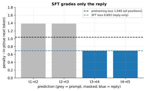
Reading it: each bar is one next-token prediction from the worked example, and its height is the penalty −ln p. Grey bars predict prompt tokens and are masked out of the SFT loss; blue bars predict reply tokens and are the only ones that count. The dashed lines mark the two averages: 1.040 over everything (pretraining) and 0.693 over the reply (SFT).
In code: response_mask builds the true/false list of graded
predictions, and sft_loss averages per_position_losses over only the
positions it marks.
Why it matters in practice. SFT needs far less data than pretraining (thousands to hundreds of thousands of examples) and quality beats quantity: a few thousand excellent examples outperform a mountain of mediocre ones. If you fine-tune your own model and forget the mask, it learns to write user prompts too.
3. Preference tuning: a taste test instead of a recipe
Everyday picture. It is hard to write down the perfect answer, but easy to taste two dishes and say which is better. Preference tuning collects exactly those judgements: people (or a model following written principles) compare two responses and pick one.
3a. RLHF: train a critic, then train the cook against it
A reward model learns to predict those judgements, giving each response a score. Reinforcement learning then tunes the language model to earn high scores. The link between scores and "which one wins" is the Bradley-Terry model, built on the sigmoid function σ(z) = 1 / (1 + e^−z), which squashes any number into a probability between 0 and 1 (σ(0) = 0.5, σ(2) = 0.881).
Tiny worked example. The reward model scores the chosen answer 3.0 and the rejected one 1.0. The gap is 2, so it predicts the chosen answer wins with probability σ(2) = 0.881, and its loss on this pair is −ln 0.881 = 0.127. Had it scored both 1.0, it would predict a coin flip (0.5) and pay ln 2 = 0.693.
flowchart LR
  PR[Prompt] --> LM[Language model]
  LM --> RA[Response A] & RB[Response B]
  RA & RB --> H[Human or AI labeler<br/>picks the better one]
  H --> RM[Reward model<br/>learns to score responses]
  RM --> RL[Reinforcement learning<br/>tune the LM to score high]
  RL --> LM
Reading it: the loop has two learners. First, labelers compare pairs and the reward model learns to agree with them. Second, the language model generates new responses, the reward model scores them, and reinforcement learning (usually PPO) nudges the language model towards higher scores, with a penalty for drifting far from where it started. Two models, two training runs, lots of moving parts.
Level 3: the formula and its symbols
$$ P(y_w \succ y_l) = \sigma\big(r(y_w) - r(y_l)\big) \qquad \mathcal{L}_{\text{RM}} = -\log \sigma\big(r(y_w) - r(y_l)\big) $$
Symbols
| Symbol | Meaning here | Shape / range |
|---|---|---|
| $y_w, y_l$ | the preferred ("winning") and rejected ("losing") responses | text |
| $\succ$ | "is preferred to" | |
| $r(y)$ | the reward model's score for response y | any real number |
| $\sigma(z)$ | sigmoid, $1/(1+e^{-z})$: turns a score gap into a probability | 0 … 1 |
| $e$ | Euler's number, 2.718…; $e^{-z}$ is "e to the power −z" | |
| $\mathcal{L}_{\text{RM}}$ | the reward model's loss on this pair | ≥ 0 |
In words: the chance the preferred answer wins is the sigmoid of the score gap, and the reward model is penalised by minus the log of the probability it gave to the choice people actually made.
On the worked example: r(y_w) = 3, r(y_l) = 1, gap 2, σ(2) = 0.881, loss −ln 0.881 = 0.127.
Level 3: in Python
In Python:
import math
def sigma(z):
    return 1 / (1 + math.exp(-z))
r_w, r_l = 3.0, 1.0
# P(y_w ≻ y_l)
round(sigma(r_w - r_l), 3)  # → 0.881
# L_RM
round(-math.log(sigma(r_w - r_l)), 3)  # → 0.127
# equal scores: a coin flip, ln 2
round(-math.log(sigma(1.0 - 1.0)), 3)  # → 0.693
In code: sigmoid squashes a score gap into a probability,
preference_probability applies it to two rewards (the Bradley-Terry
model), and reward_model_loss is minus the log of that probability.
3b. DPO: skip the critic
Everyday picture. Instead of hiring a food critic and cooking to please them, edit the recipe book directly from the taste-test results, while keeping a copy of the original book so you don't drift too far from it.
Tiny worked example. A log-probability is the log of the probability the model gives a whole response (a sum of per-token log probabilities; more negative means less likely). The frozen reference model gives both answers −11. After some training the policy gives the chosen answer −10 (more likely than before) and the rejected one −12 (less likely). With β = 0.1 the margin is 0.1 × ((−10 − −11) − (−12 − −11)) = 0.1 × (1 + 1) = 0.2; the loss is −ln σ(0.2) = 0.598, down from ln 2 = 0.693 when the policy still equalled the reference.
flowchart LR
  PAIR[Preference pair<br/>chosen, rejected] --> POL[Policy being trained<br/>log π of each]
  PAIR --> REF[Frozen reference<br/>log π_ref of each]
  POL --> M[Margin = β × how much more the policy<br/>boosted chosen than rejected]
  REF --> M
  M --> LOSS[−log σ margin]
  LOSS -->|gradient| POL
Reading it: each preference pair is scored twice: by the model being trained and by a frozen copy of where it started. The margin measures how much more the policy has boosted the chosen answer than the rejected one, relative to the reference. The loss is the reward-model loss again, but the "reward" is read straight off the policy's own probabilities, so there is no separate reward model and no reinforcement-learning loop.
Level 3: the formula and its symbols
$$ \mathcal{L}_{\text{DPO}} = -\log \sigma\Big(\beta\big[(\log\pi_\theta(y_w) - \log\pi_{\text{ref}}(y_w)) - (\log\pi_\theta(y_l) - \log\pi_{\text{ref}}(y_l))\big]\Big) $$
Symbols
| Symbol | Meaning here | Shape / range |
|---|---|---|
| $\pi_\theta(y)$ | the policy: the model being trained, with weights θ; π(y) is the probability it gives response y | 0 … 1 |
| $\pi_{\text{ref}}(y)$ | the frozen reference model (usually the SFT model) | 0 … 1 |
| $\log\pi_\theta(y) - \log\pi_{\text{ref}}(y)$ | the log-ratio: how much more likely training has made y. β times it is the implicit reward $\hat r(y)$, so the bracket scaled by β is $\hat r(y_w) - \hat r(y_l)$ | any real |
| $\beta$ | beta, the leash to the reference: it sets how much a change in log-probability counts, so a larger β satisfies the loss with a smaller departure and keeps the policy closer to the reference; a smaller β lets the preferences pull it further away | typically 0.1 to 0.5 |
| $\sigma$, $\log$ | sigmoid and natural log, as above |
In words: raise the probability of the chosen answer and lower the rejected one, measured relative to the frozen starting model, and penalise the model by minus the log-sigmoid of that scaled gap.
On the worked example: β = 0.1, log-ratios +1 (chosen) and −1 (rejected), so implicit rewards r̂ = 0.1 × 1 = +0.1 and 0.1 × (−1) = −0.1, margin 0.1 − (−0.1) = 0.2, σ(0.2) = 0.550, loss 0.598. The gradient's size is β × (1 − σ(margin)) = 0.1 × 0.450 = 0.045: pairs the policy already ranks correctly get gentle updates, and pairs it ranks the wrong way get strong ones.
Level 3: in Python
In Python:
import math
def sigma(z):
    return 1 / (1 + math.exp(-z))
beta = 0.1
# chosen answer: policy, reference
logpi_w, logpi_ref_w = -10.0, -11.0
# rejected answer: policy, reference
logpi_l, logpi_ref_l = -12.0, -11.0
# implicit rewards r̂ = β × log-ratio
r_w = beta * (logpi_w - logpi_ref_w)
r_l = beta * (logpi_l - logpi_ref_l)
print(f"{r_w:.1f} {r_l:.1f}")  # → 0.1 -0.1
margin = r_w - r_l
print(f"{margin:.1f} {sigma(margin):.3f}")  # → 0.2 0.550
# L_DPO
round(-math.log(sigma(margin)), 3)  # → 0.598
# how hard this pair pushes
round(beta * (1 - sigma(margin)), 3)  # → 0.045
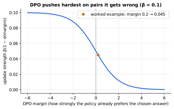
Reading it: the x-axis is the DPO margin (how strongly the policy already prefers the chosen answer, relative to the reference); the y-axis is how hard one gradient step pushes. Far left, the policy has the pair backwards and gets the full push, β. At zero (no preference yet) it gets half. Far right, the pair is learned and updates fade to nothing, so training effort flows automatically to the pairs still wrong.
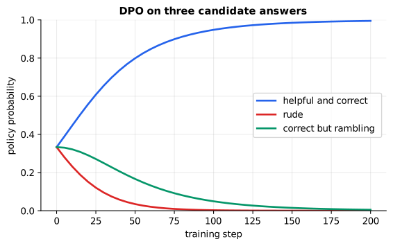
Reading it: a one-prompt toy policy starts uniform over three answers (1/3 each). The preference data says "helpful and correct" beats both others and "correct but rambling" beats "rude". As training steps pass (x-axis), probability (y-axis) flows to the top answer, the rude answer is pushed down fastest, and the rambling answer falls too but more slowly (0.166 at step 50, 0.005 by step 200), staying above rude the whole way: the ordering people expressed. Nothing here stops the top answer taking nearly everything, because every pair it appears in keeps pushing it up.
In code: dpo_margin computes the gap between implicit rewards
(β times each log-ratio), dpo_loss turns it into −log σ(margin), and dpo_update_strength
gives the push β × (1 − σ(margin)) plotted in the first figure;
train_toy_dpo trains the three-answer toy policy of the second.
Why it matters in practice. DPO is simpler and more stable than RLHF, which is why it is widely used in open-model fine-tuning. Constitutional AI and AI-feedback methods scale the labelling by having a model judge responses against written principles. This stage is where tone, helpfulness, refusals and safety behaviour mostly come from.
4. LoRA: sticky notes instead of reprinting the textbook
Everyday picture. You want to adapt a 1,000-page textbook for your class. Reprinting it is expensive. Instead you add a small stack of sticky notes with corrections. The book stays untouched; the notes are cheap to write, store and swap, and you can photocopy them into the book when you're done.
Tiny worked example. Frozen weights W = the 2×2 identity (it copies its input). Adapter B = (1, 0) as a column and A = (0, 1) as a row. For input x = (1, 2): the frozen path gives W·x = (1, 2). The adapter first squeezes x to one number, A·x = 2, then expands it back, B·2 = (2, 0). The output is (1, 2) + (2, 0) = (3, 2). Two small vectors changed the layer's behaviour without touching W.
flowchart LR
  X[input x<br/>d numbers] --> W[W, frozen<br/>d × d]
  X --> A[A, trainable<br/>squeeze to r numbers]
  A --> B[B, trainable, starts at 0<br/>expand back to d]
  W --> ADD((+))
  B --> ADD
  ADD --> Y[output y]
Reading it: the input takes two paths. The top path is the pretrained layer, which never changes. The bottom path is the adapter: A squeezes the d-dimensional input down to a tiny rank r (say 8), and B expands it back. Because B starts at zero, the bottom path adds nothing at first and the model starts exactly where pretraining left it. Only A and B are trained. Afterwards you can add B·A into W once ("merge") and serve the model at exactly the original speed.
Level 3: the formula and its symbols
$$ y = xW^\top + \frac{\alpha}{r}\, x A^\top B^\top \qquad \text{trainable parameters} = r\,d_{\text{in}} + d_{\text{out}}\,r $$
Symbols
| Symbol | Meaning here | Shape / range |
|---|---|---|
| $x$ | input row vector | (d_in,) |
| $W$ | frozen pretrained weight matrix | (d_out, d_in) |
| $^\top$ | transpose: flip rows and columns so the shapes line up for multiplication | |
| $A$ | trainable "down" matrix, random at start | (r, d_in) |
| $B$ | trainable "up" matrix, zero at start | (d_out, r) |
| $r$ | the rank: the width of the bottleneck | usually 4 to 64 |
| $\alpha$ | alpha, a scale knob; α/r keeps update size steady when you change r | often r or 2r |
In words: the output is what the frozen layer produces plus a scaled correction that passes through a narrow r-number bottleneck.
On the worked example: W = I, A = (0, 1), B = (1, 0)ᵀ, α/r = 1, x = (1, 2): xWᵀ = (1, 2), xAᵀ = 2, 2·Bᵀ = (2, 0), y = (3, 2).
Level 3: in Python
In Python:
# x Mᵀ: the dot product of x with each row of M
def times_transpose(x, M):
    return [sum(x_k * m_k for x_k, m_k in zip(x, row)) for row in M]
# frozen, d_out × d_in
W = [[1, 0], [0, 1]]
# r × d_in, with r = 1
A = [[0, 1]]
# d_out × r
B = [[1], [0]]
x, alpha_over_r = [1, 2], 1
# x Wᵀ
frozen = times_transpose(x, W)
# x Aᵀ: squeezed to r numbers
squeezed = times_transpose(x, A)
# (x Aᵀ) Bᵀ: expanded back
correction = times_transpose(squeezed, B)
frozen, squeezed, correction  # → ([1, 2], [2], [2, 0])
# y
[f_j + alpha_over_r * c_j for f_j, c_j in zip(frozen, correction)]  # → [3, 2]
d_in = d_out = 4096
# full, then LoRA at each rank
d_out * d_in, [r * d_in + d_out * r for r in (64, 16, 8)]  # → (16777216, [524288, 131072, 65536])
Parameter savings for one 4096 × 4096 layer:
| Method | Trainable parameters | Share of full |
|---|---|---|
| full fine-tune | 16,777,216 | 100% |
| LoRA r = 64 | 524,288 | 3.1% |
| LoRA r = 16 | 131,072 | 0.78% |
| LoRA r = 8 | 65,536 | 0.39% |
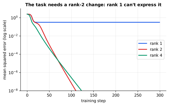
Reading it: the task needs a rank-2 change to a frozen 16 × 16 layer. The y-axis (log scale) is the training error; the x-axis is the training step. A rank-1 adapter plateaus: its bottleneck is too narrow to express the change. Ranks 2 and 4 drive the error to essentially zero. This is the LoRA bet: the change a fine-tune needs is low-rank even though the weights themselves are not.
In code: LoRALinear holds the frozen W beside the trainable A and B,
and LoRALinear.merged_weight folds the adapter into W for serving.
lora_trainable_params and full_trainable_params count the table's
parameters, and train_toy_lora trains the adapters in the figure.
QLoRA goes further: it stores the frozen base weights in 4 bits (a format called NF4) and trains LoRA adapters in 16-bit on top, which lets a 65-billion-parameter model be fine-tuned on a single 48 GB GPU.
Why it matters in practice. LoRA adapters are megabytes, not gigabytes. You can keep one per customer or task and hot-swap them on one shared base model, and training fits on far smaller hardware.
5. Which adaptation should you use?
Everyday picture. If a new employee doesn't know your product catalogue, you hand them the catalogue (retrieval); you don't send them back to school. If they know the facts but write emails in the wrong tone, you first give clearer instructions, then coach them, and only for a whole new profession do you retrain from scratch.
| Approach | Changes weights? | Use when |
|---|---|---|
| Prompting / few-shot | No | behaviour or format change |
| RAG | No | knowledge that changes or must be cited |
| LoRA / QLoRA | small adapters | style, domain vocabulary, consistent output format |
| Full fine-tune | yes, all | rarely: major domain shift with lots of data |
flowchart TD
  Q1{Missing knowledge,<br/>or facts that change?} -->|Yes| R[Use RAG]
  Q1 -->|No| Q2{Wrong behaviour,<br/>format or tone?}
  Q2 -->|No| N[No change needed]
  Q2 -->|Yes| P[Improve the prompt<br/>add examples]
  P -->|Still inconsistent<br/>or too costly| L[LoRA fine-tune]
  L -->|Major domain shift,<br/>lots of data| F[Full fine-tune]
Reading it: start at the top. Knowledge problems exit immediately to retrieval. Behaviour problems climb a ladder of cost and only go as far as they must: prompt first, a LoRA adapter if the prompt can't make the behaviour consistent (or the prompt is too long and costly to send every time), and a full fine-tune only for a genuine domain shift with lots of data.
In code: choose_adaptation walks this flowchart, cheapest option
first, and returns the approach it lands on.
The key line: fine-tuning teaches behaviour; RAG supplies knowledge. Most production systems end up as retrieval plus a well-built prompt.
6. Distillation: the apprentice learns how the master hesitates
Everyday picture. A master chef tastes a sauce and says "mostly thyme, a bit of rosemary, definitely not mint". An apprentice who only hears "thyme" learns less than one who hears the whole judgement. Distillation trains a small, cheap student model to match a big teacher's full probability spread, not just its top answer.
Tiny worked example. The teacher's raw scores (logits) for three answers are 2, 1, 0. Softmax at temperature T = 1 gives 0.665, 0.245, 0.090. Dividing the logits by T = 2 first gives softmax(1, 0.5, 0) = 0.506, 0.307, 0.186: flatter, so the student clearly sees that answer 2 is a much better runner-up than answer 3. That runner-up information is sometimes called "dark knowledge".
flowchart LR
  X[Same input] --> T[Big teacher model]
  X --> S[Small student model]
  T --> TS[softmax of logits / T<br/>soft targets]
  S --> SS[softmax of logits / T]
  TS --> KL[KL divergence<br/>how different are they?]
  SS --> KL
  KL -->|gradient| S
Reading it: both models see the same input. Each one's scores are softened by the same temperature, and the KL divergence measures how far the student's spread is from the teacher's. Only the student learns; the teacher is fixed. Typically this runs over large volumes of the exact traffic your product sees, so the student becomes an expert at your task.
Level 3: the formula and its symbols
$$ p_i^{(T)} = \frac{e^{z_i/T}}{\sum_j e^{z_j/T}} \qquad \mathrm{KL}(p \,\|\, q) = \sum_i p_i \ln\frac{p_i}{q_i} \qquad \mathcal{L} = \alpha\,T^2\,\mathrm{KL}\big(p^{(T)} \,\|\, q^{(T)}\big) + (1-\alpha)\,\mathrm{CE} $$
Symbols
| Symbol | Meaning here | Shape / range |
|---|---|---|
| $z_i$ | the teacher's logit (raw score) for answer i | any real |
| $T$ | temperature: divide scores by T before softmax; T > 1 flattens | > 0 |
| $p^{(T)}, q^{(T)}$ | teacher and student probabilities at temperature T | each sums to 1 |
| $\mathrm{KL}(p|q)$ | Kullback-Leibler divergence: the extra surprise from believing q when the truth is p. Zero only when they match | ≥ 0 |
| $\ln$ | natural logarithm | |
| $T^2$ | rescales the gradient, which softening shrinks by 1/T² | |
| $\alpha$ | mix between matching the teacher and matching the true label | 0 … 1 |
| CE | ordinary cross-entropy on the true label | ≥ 0 |
In words: the student is penalised by how far its softened spread is from the teacher's, scaled by T², optionally mixed with the usual penalty on the true answer.
On the worked example: with teacher (0.5, 0.5) and student (0.9, 0.1), KL = 0.5·ln(0.5/0.9) + 0.5·ln(0.5/0.1) = −0.294 + 0.805 = 0.511. When the student matches the teacher exactly, KL = 0. If those are the two spreads at T = 2 and α = 1 (learn from the teacher alone), the loss is 2² × 0.511 = 2.04.
Level 3: in Python
In Python:
import math
def soft_targets(z, T):
    # e^(z_i / T)
    exps = [math.exp(z_i / T) for z_i in z]
    # divided by Σ_j e^(z_j / T)
    return [e / sum(exps) for e in exps]
[round(p_i, 3) for p_i in soft_targets([2, 1, 0], T=2)]  # → [0.506, 0.307, 0.186]
# teacher, student
p, q = [0.5, 0.5], [0.9, 0.1]
KL = sum(p_i * math.log(p_i / q_i) for p_i, q_i in zip(p, q))
round(KL, 3)  # → 0.511
alpha, T = 1.0, 2
# the (1 − α)·CE term is zero at α = 1
round(alpha * T ** 2 * KL, 2)  # → 2.04
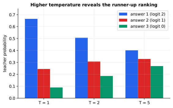
Reading it: the same three teacher logits (2, 1, 0) shown at three temperatures. At T = 1 (left group) the top answer dominates. At T = 2 and T = 5 the bars even out and the ranking of the wrong answers becomes visible to the student. Too high a temperature and everything flattens to a uniform guess, so T is tuned (2 to 5 is common).
In code: soft_targets divides logits by T and applies softmax,
kl_divergence measures how far apart two spreads are, and
distillation_loss combines them with the T² scale and the optional
cross-entropy on the true label.
Why it matters in practice. Distillation is often the biggest cost lever in production: a small student trained on a big model's outputs for one narrow task can be many times cheaper and faster with little quality loss on that task.
In 20 seconds
- Pretraining predicts the next token over huge text and gives knowledge; SFT teaches the assistant format; preference tuning shapes tone, helpfulness and safety.
- SFT is next-token loss with the prompt masked out.
- RLHF trains a reward model on pairwise preferences, then optimises the LM against it; DPO gets the same effect directly from preference pairs.
- LoRA trains a tiny low-rank correction B·A beside frozen weights: 0.39% of a layer's parameters at rank 8, 3.1% at rank 64, mergeable for zero added latency.
- Fine-tuning teaches behaviour; RAG supplies knowledge. Start with prompting and RAG.
- Distillation trains a small student on a big teacher's soft targets; it's a major cost lever.
Self-test questions
Q: Why does a base model ramble instead of answering? A: Pretraining only teaches it to continue text. Answering questions in a helpful format is learned later, in SFT and preference tuning.
Q: What is the one code difference between pretraining loss and SFT loss? A: A mask. SFT computes the same next-token cross-entropy but averages it only over the reply tokens, so the prompt is read but not trained on.
Q: In RLHF, what does the reward model learn, and from what? A: A score for responses such that sigmoid(score gap) predicts which of two responses a labeler preferred. It learns from pairwise comparisons, which are far easier for people to give than perfect answers.
Q: How does DPO avoid a reward model? A: It treats the log-probability ratio between the policy and a frozen reference as an implicit reward, and applies the same pairwise loss directly to the policy. One model, one supervised-style training loop.
Q: What does β control in DPO? A: How tightly the policy is held to the reference model. It is the weight on the drift penalty in the objective DPO optimises, reward − β × KL(policy ‖ reference), so larger β keeps the policy closer to the reference and smaller β lets the preferences pull it further away. In the loss, a larger β makes each unit of log-ratio count for more, so pairs are satisfied with a smaller departure.
Q: Why is B initialised to zero in LoRA? A: So B·A = 0 and the adapted model starts exactly equal to the pretrained model. Training then learns only the change.
Q: How many parameters does LoRA rank 8 train on a 4096 × 4096 layer? A: 2 × 4096 × 8 = 65,536, about 0.39% of the 16.8 million in the full matrix.
Q: Does LoRA slow down inference? A: Not if you merge: add B·A into W once and serve the result. Unmerged adapters cost two thin extra matmuls, which is what lets you hot-swap adapters on one base model.
Q: A client wants the model to know their product catalogue, which changes weekly. Fine-tune or RAG? A: RAG. The knowledge changes and answers should cite sources; fine-tuning would be stale within a week and can't cite. Fine-tune only for behaviour the prompt can't make consistent.
Q: What does temperature do in distillation? A: It softens both distributions so the student learns the teacher's relative preferences among wrong answers, not just its top pick; the T² factor keeps gradient sizes comparable.
The papers behind this lesson
- Brown et al., Language Models are Few-Shot Learners (GPT-3, 2020): https://arxiv.org/abs/2005.14165. Showed that scaling next-token pretraining produces a model that can follow instructions and examples given only in the prompt. annotated companion
- Kaplan et al., Scaling Laws for Neural Language Models (2020): https://arxiv.org/abs/2001.08361, with Hoffmann et al., Training Compute-Optimal Large Language Models (2022): https://arxiv.org/abs/2203.15556. Measured how pretraining loss falls predictably with model size, data and compute, and how to balance them. annotated companion
- Ouyang et al., Training language models to follow instructions with human feedback (InstructGPT, 2022): https://arxiv.org/abs/2203.02155. Established the SFT, reward model and RLHF recipe behind chat assistants. annotated companion
- Rafailov et al., Direct Preference Optimization: Your Language Model is Secretly a Reward Model (2023): https://arxiv.org/abs/2305.18290. Showed preference tuning can skip the reward model and RL loop entirely. annotated companion
- Hu et al., LoRA: Low-Rank Adaptation of Large Language Models (2021): https://arxiv.org/abs/2106.09685, with Dettmers et al., QLoRA (2023): https://arxiv.org/abs/2305.14314. Fine-tuned huge models by training small low-rank adapters beside frozen (and, in QLoRA, 4-bit) weights. annotated companion
- Hinton, Vinyals & Dean, Distilling the Knowledge in a Neural Network (2015): https://arxiv.org/abs/1503.02531. Trained small students on a large teacher's temperature-softened outputs. annotated companion
- Bai et al., Constitutional AI: Harmlessness from AI Feedback (2022): https://arxiv.org/abs/2212.08073. Replaced much human preference labelling with a model judging responses against written principles.
Further reading
- Hugging Face PEFT documentation: https://huggingface.co/docs/peft/index
- Hugging Face TRL documentation (SFT, DPO, reward modelling): https://huggingface.co/docs/trl/index
1r""" 2# Training stages: how a text predictor becomes an assistant 3 4Run: `python -m primer.ml.training_stages` 5 6New to the notation? `primer.notation` explains every symbol used here 7(Σ, log, σ, subscripts, ᵀ, and so on) from zero. 8 9## Level 1: The practitioner's guide 10 11**In one sentence.** An assistant model is built in stages (pretraining for 12knowledge, supervised fine-tuning for the assistant format, preference 13tuning for tone and safety), and knowing which stage produced a behaviour 14tells you which lever (a prompt, retrieval, a small adapter, a full 15fine-tune) will change it. 16 17**When you need it.** You need this map the first time a model does 18something you cannot fix by rewording the prompt, and the question becomes 19"do we fine-tune?". The tell: a behaviour that stays wrong across many 20prompt rewrites (the house style never quite lands, the output format is 21right 95 times in 100 and you need 100), or a system prompt so long that 22sending it with every call is most of your bill. You don't need training 23when the model lacks a fact: a base model's knowledge is frozen at its 24training date (the knowledge cutoff), so a product catalogue that changes 25weekly is a retrieval problem, not a training problem. You also don't need it when a 26clearer instruction or two examples in the prompt already fix the behaviour. 27Most production systems end up as retrieval plus a well-built prompt. 28 29**Your options.** From the cheapest to the most committed: 30 31| Option | What it does | What it guarantees | What it costs | Where it lives | 32|---|---|---|---|---| 33| Prompting and few-shot examples | Describe the behaviour, show one or two examples | Nothing; it raises the odds, and the vendor's SFT and preference tuning did the heavy lifting | Extra input tokens on every call | Your prompt | 34| Retrieval (RAG) | Fetch the facts at request time and put them in the prompt | Current, citable knowledge | An index to build and keep fresh, longer prompts | Your code | 35| Hosted supervised fine-tuning | Train the vendor's model on your prompt-and-reply pairs; only the reply is graded | Consistent format and style without the long prompt | Curated examples, a training job, sometimes a higher per-token price | The vendor's fine-tuning API | 36| LoRA or QLoRA adapter | Train a small low-rank correction beside frozen weights of an open model | Same effect as a fine-tune while training a few percent of the parameters or less (0.39% of a layer at rank 8, 3.1% at rank 64); mergeable for no added latency | A GPU you rent or own, data, a model to serve | Your training and serving stack | 37| Preference tuning (DPO) on your own pairs | Show chosen-versus-rejected pairs; the model learns to prefer the chosen kind | Shifts tone, verbosity and refusals that no single "correct answer" captures | Thousands of comparisons, a frozen reference copy, one training loop | Your training stack, or a hosted API that offers it | 38| Full fine-tune | Update every weight on a large dataset | The largest possible shift: a new domain, a new language | Multi-GPU training, a copy of the whole model per variant, real risk of forgetting | Your training stack | 39| Distillation | Train a small student to imitate a big teacher's full probability spread on your traffic | A cheaper, faster model for one narrow task | Millions of teacher outputs, a training run, an eval suite | Your training stack | 40 41**How to choose.** The lesson's `choose_adaptation` walks this order, 42cheapest first, and stops at the first lever that fits. 43 44- Missing or changing knowledge, or answers that must cite a source: 45 retrieval. Fine-tuned knowledge is stale the day the data changes and 46 cannot point at where it came from. 47- Wrong behaviour, format or tone: improve the prompt and add examples. 48 Stop here if it works. 49- Still inconsistent with a good prompt, or the prompt is too long to send 50 every time: a LoRA adapter (or the hosted equivalent). A few thousand 51 excellent examples beat a mountain of mediocre ones; LIMA (Zhou et al., 52 2023) fine-tuned a 65-billion-parameter model on 1,000 curated examples. 53- A judgement no reference answer captures (which of two drafts is better): 54 preference tuning with DPO, which needs no reward model and no 55 reinforcement-learning loop. 56- A genuine domain shift with millions of examples: a full fine-tune, and 57 only then. 58- Too expensive at volume: distil the working big model into a small one for 59 that task. 60- Whatever you pick, fine-tuning teaches behaviour and retrieval supplies 61 knowledge. Hold an evaluation set out before you train anything, because 62 every stage past prompting can quietly make something else worse. 63 64**What it costs.** Prompting costs tokens, on every call, forever. 65Retrieval costs an index and longer prompts. Fine-tuning costs data first: 66supervised fine-tuning needs thousands to hundreds of thousands of examples 67(this lesson), and each one must be an answer you would be happy to see a 68thousand times. Compute is smaller than people expect once weights are 69frozen: for one 4096 × 4096 layer, a full fine-tune trains 16,777,216 70parameters, a rank-8 LoRA adapter trains 65,536 (0.39%), and the adapter is 71megabytes rather than gigabytes (this lesson's `lora_trainable_params`). 72The LoRA paper reports up to 10,000 times fewer trainable parameters and 73three times less GPU memory than full fine-tuning at the same quality; QLoRA 74stores the frozen base in 4 bits and fine-tunes a 65-billion-parameter model 75on one 48 GB GPU in 24 hours. Merged, an adapter adds no serving latency. 76Pretraining is the one stage you never pay for directly: months of 77multi-GPU time, and a vendor's model card is how its cost reaches you as 78knowledge cutoff, languages covered and coding ability. 79 80**What breaks.** 81 82- **Training on the prompt.** Forget the mask that grades only the reply and 83 the model learns to write user questions too. Hosted APIs mask for you; if 84 you write the loop, `response_mask` is the whole difference. 85- **Fine-tuning for facts.** The model learns the phrasing of your documents 86 more than their content, and is out of date at the next edit. Retrieve. 87- **A rank too small.** In the lesson's toy, a rank-1 adapter plateaus on a 88 task that needs rank 2 while ranks 2 and 4 drive the error to zero. If an 89 adapter stalls, raise r before blaming the data. 90- **Preference tuning that collapses.** The lesson's DPO toy pushes the top 91 answer to 0.995 and everything else to nearly zero, because every pair the 92 winner appears in keeps pushing it up. A larger β keeps the model closer 93 to its starting point; watch for a model that says one thing every time. 94- **Forgetting.** Any fine-tune shifts skills you did not train on. Keep a 95 general evaluation beside your task evaluation. 96- **Base versus instruct.** Fine-tuning a base model gives you a base model 97 that continues text; start from the instruction-tuned checkpoint unless you 98 are prepared to redo SFT yourself. 99 100**In the wild.** The vendor's side of the pipeline is the InstructGPT 101recipe (Ouyang et al., 2022): supervised fine-tuning, a reward model, then 102reinforcement learning; that paper found a 1.3-billion-parameter model 103tuned this way preferred over the 175-billion-parameter GPT-3 it started 104from. Hosted fine-tuning APIs expose supervised fine-tuning and, at some 105vendors, DPO and reinforcement fine-tuning with a grader (OpenAI's model 106optimization guide lists all three). For open models, Hugging Face TRL 107provides SFTTrainer, RewardTrainer, DPOTrainer, GRPOTrainer and a 108DistillationTrainer; PEFT provides LoRA and its relatives; and vLLM 109serves many LoRA adapters on one base model, picking the adapter per request 110(a LoRARequest, bounded by max_loras), which is how one shared server 111carries a fine-tune per customer. The papers are linked at the end of the 112lesson. 113 114**Go deeper.** Level 2 builds each stage in a few lines: the next-token loss 115and the one mask that turns it into SFT, a reward model as a taste test, DPO 116as the same loss read off the policy itself, a LoRA layer you can multiply 117out by hand, and distillation's softened targets, each with a figure you can 118rerun. If you only needed to choose a lever, you are done. 119 120## Level 2: How it works, from scratch 121 122A chat assistant is built in layers, and each layer explains a different 123behaviour you see: 124 125```mermaid 126flowchart LR 127 P[Pretraining<br/>guess the next token<br/>over web-scale text] --> B[Base model<br/>knows a lot, rambles] 128 B --> S[SFT<br/>study examples of<br/>good answers] 129 S --> PT[Preference tuning<br/>RLHF or DPO] 130 PT --> A[Assistant model] 131 A --> D[Your adaptation<br/>prompts, RAG, LoRA] 132``` 133 134**Reading it:** read left to right; each box is a training stage and each 135arrow hands a model to the next stage. The model *vendor* runs the first 136three stages: pretraining (months, millions of dollars) gives a base model 137that knows facts but just continues text; supervised fine-tuning (SFT) 138teaches it the *format* of being an assistant; preference tuning shapes tone, 139helpfulness and safety. You work in the last box. When a model knows a fact 140it learned that in pretraining; when it answers in tidy bullet points it 141learned that in SFT and preference tuning. 142 143This lesson builds a small, real version of every stage: the pretraining 144and SFT losses, a reward model, DPO, LoRA, the "which adaptation?" decision, 145and distillation. 146 147## 1. Pretraining: guess the next word, a trillion times 148 149**Everyday picture.** Imagine reading every book in a library with a card 150covering the next word, guessing it, then sliding the card to check. Do 151that trillions of times and you absorb grammar, facts, arithmetic habits and 152coding conventions, because every one of them helps you guess the next word. 153 154**Tiny worked example.** A 5-token sequence gives 4 guesses (token 1 155predicts token 2, and so on; the last token has nothing after it to check). 156Suppose the model gave the right next token probability 0.25, 0.25, 0.5 and 1570.5. The penalty for each guess is −ln(probability): 1.386, 1.386, 0.693, 1580.693. The pretraining loss is their average, **1.040**. 159 160```mermaid 161flowchart LR 162 T1[t1] --> G1{guess t2} 163 T2[t2] --> G2{guess t3} 164 T3[t3] --> G3{guess t4} 165 T4[t4] --> G4{guess t5} 166 G1 & G2 & G3 & G4 --> AVG[average of −ln p<br/>= the loss] 167``` 168 169**Reading it:** every position makes one guess about the token that follows 170it, using only what came before. The model is scored on all guesses at 171once and the average penalty is the number training pushes down. One text 172sequence of n tokens therefore gives n − 1 training examples for free, which 173is why unlabeled text is such a rich training signal. 174 175$$ 176\mathcal{L}_{\text{pretrain}} = -\frac{1}{n-1}\sum_{i=1}^{n-1} \log p_\theta(t_{i+1} \mid t_{1..i}) 177$$ 178 179**Symbols** 180 181| Symbol | Meaning here | Shape / range | 182|---|---|---| 183| $\mathcal{L}_{\text{pretrain}}$ | the loss: one number, lower is better | ≥ 0 | 184| $n$ | number of tokens in the sequence | integer | 185| $\Sigma_{i=1}^{n-1}$ | add up the term for every position i from 1 to n−1 | | 186| $t_{i}$ | the i-th token (an integer id) | 0 … vocab−1 | 187| $t_{1..i}$ | all tokens up to and including position i (the context) | | 188| $p_\theta(t_{i+1} \mid t_{1..i})$ | probability the model with weights θ gives the true next token, given the context. The bar "∣" reads "given" | 0 … 1 | 189| $\theta$ | all the model's weights | millions to trillions of numbers | 190| $\log$ | natural logarithm. ln 1 = 0 and ln of a small number is very negative, so −log turns "probability of being right" into "penalty" | | 191 192**In words:** the loss is the average, over every position, of minus the 193log of the probability the model gave to the token that actually came next. 194 195**On the worked example:** n = 5, the four probabilities are 0.25, 0.25, 1960.5, 0.5, so the loss is −(ln 0.25 + ln 0.25 + ln 0.5 + ln 0.5) / 4 = 197(1.386 + 1.386 + 0.693 + 0.693) / 4 = 1.040. 198 199**In Python:** 200 201```python 202import math 203# p_θ(t_{i+1} | t_{1..i}) for each of the guesses 204p = [0.25, 0.25, 0.5, 0.5] 205# 5 tokens give n − 1 = 4 guesses 206n = len(p) + 1 207[round(-math.log(p_i), 3) for p_i in p] # → [1.386, 1.386, 0.693, 0.693] 208L_pretrain = -sum(math.log(p_i) for p_i in p) / (n - 1) 209print(f"{L_pretrain:.3f}") # → 1.040 210``` 211 212**In code:** `per_position_losses` computes −ln p for every next-token guess 213(with a stable `log_softmax`), and `next_token_loss` averages them into the 214pretraining loss. 215 216**Why it matters in practice.** Pretraining is where knowledge comes from, 217and it is frozen at a date (the "knowledge cutoff"). A base model continues 218text instead of answering questions: ask "What is the capital of France?" 219and it may continue with "What is the capital of Spain?", because question 220lists are common on the web. 221 222## 2. Supervised fine-tuning (SFT): study the answers, not the questions 223 224**Everyday picture.** An apprentice studies a binder of worked examples: 225customer question, then the expert's reply. They read the question 226carefully, but they are graded only on writing the reply. Nobody marks them 227on reproducing the customer's typing. 228 229**Tiny worked example.** Same 5 tokens, but the first 3 are the prompt and 230the last 2 are the reply. Only the 2 guesses whose target is a reply token 231count: penalties 0.693 and 0.693, average **0.693**. The prompt guesses 232(1.386 each) are ignored. 233 234```mermaid 235flowchart LR 236 subgraph Prompt["prompt: read, not graded"] 237 P1[t1] --> P2[t2] --> P3[t3] 238 end 239 subgraph Reply["reply: graded"] 240 R1[t4] --> R2[t5] 241 end 242 P3 --> R1 243 R1 -.->|loss| L[average −ln p<br/>over reply tokens only] 244 R2 -.->|loss| L 245``` 246 247**Reading it:** the whole sequence flows through the model, so the reply is 248conditioned on the prompt. The dotted arrows show which predictions reach 249the loss: only those that produce reply tokens. That mask (a list of 250true/false per position) is the whole difference between pretraining code 251and SFT code. 252 253$$ 254\mathcal{L}_{\text{SFT}} = -\frac{\sum_{i} m_i \,\log p_\theta(t_{i+1} \mid t_{1..i})}{\sum_i m_i} 255$$ 256 257**Symbols** 258 259| Symbol | Meaning here | Shape / range | 260|---|---|---| 261| $m_i$ | the mask: 1 if token i+1 belongs to the reply, else 0 | 0 or 1 | 262| $\sum_i m_i$ | how many predictions are graded (the reply length) | integer | 263| everything else | as in the pretraining formula | | 264 265**In words:** average the next-token penalty over the reply tokens only. 266 267**On the worked example:** m = (0, 0, 1, 1), so the loss is 268(0.693 + 0.693) / 2 = 0.693. 269 270**In Python:** 271 272```python 273import math 274p = [0.25, 0.25, 0.5, 0.5] 275# 1 only where the target is a reply token 276m = [0, 0, 1, 1] 277L_SFT = -sum(m_i * math.log(p_i) for m_i, p_i in zip(m, p)) / sum(m) 278round(L_SFT, 3) # → 0.693 279``` 280 281 282 283**Reading it:** each bar is one next-token prediction from the worked 284example, and its height is the penalty −ln p. Grey bars predict prompt 285tokens and are masked out of the SFT loss; blue bars predict reply tokens 286and are the only ones that count. The dashed lines mark the two averages: 2871.040 over everything (pretraining) and 0.693 over the reply (SFT). 288 289**In code:** `response_mask` builds the true/false list of graded 290predictions, and `sft_loss` averages `per_position_losses` over only the 291positions it marks. 292 293**Why it matters in practice.** SFT needs far less data than pretraining 294(thousands to hundreds of thousands of examples) and quality beats quantity: 295a few thousand excellent examples outperform a mountain of mediocre ones. 296If you fine-tune your own model and forget the mask, it learns to write 297user prompts too. 298 299## 3. Preference tuning: a taste test instead of a recipe 300 301**Everyday picture.** It is hard to write down the perfect answer, but easy 302to taste two dishes and say which is better. Preference tuning collects 303exactly those judgements: people (or a model following written principles) 304compare two responses and pick one. 305 306### 3a. RLHF: train a critic, then train the cook against it 307 308A **reward model** learns to predict those judgements, giving each response 309a score. Reinforcement learning then tunes the language model to earn high 310scores. The link between scores and "which one wins" is the Bradley-Terry 311model, built on the **sigmoid** function σ(z) = 1 / (1 + e^−z), which squashes 312any number into a probability between 0 and 1 (σ(0) = 0.5, σ(2) = 0.881). 313 314**Tiny worked example.** The reward model scores the chosen answer 3.0 and 315the rejected one 1.0. The gap is 2, so it predicts the chosen answer wins 316with probability σ(2) = **0.881**, and its loss on this pair is 317−ln 0.881 = **0.127**. Had it scored both 1.0, it would predict a coin flip 318(0.5) and pay ln 2 = 0.693. 319 320```mermaid 321flowchart LR 322 PR[Prompt] --> LM[Language model] 323 LM --> RA[Response A] & RB[Response B] 324 RA & RB --> H[Human or AI labeler<br/>picks the better one] 325 H --> RM[Reward model<br/>learns to score responses] 326 RM --> RL[Reinforcement learning<br/>tune the LM to score high] 327 RL --> LM 328``` 329 330**Reading it:** the loop has two learners. First, labelers compare pairs and 331the reward model learns to agree with them. Second, the language model 332generates new responses, the reward model scores them, and reinforcement 333learning (usually PPO) nudges the language model towards higher scores, 334with a penalty for drifting far from where it started. Two models, two 335training runs, lots of moving parts. 336 337$$ 338P(y_w \succ y_l) = \sigma\big(r(y_w) - r(y_l)\big) \qquad 339\mathcal{L}_{\text{RM}} = -\log \sigma\big(r(y_w) - r(y_l)\big) 340$$ 341 342**Symbols** 343 344| Symbol | Meaning here | Shape / range | 345|---|---|---| 346| $y_w, y_l$ | the preferred ("winning") and rejected ("losing") responses | text | 347| $\succ$ | "is preferred to" | | 348| $r(y)$ | the reward model's score for response y | any real number | 349| $\sigma(z)$ | sigmoid, $1/(1+e^{-z})$: turns a score gap into a probability | 0 … 1 | 350| $e$ | Euler's number, 2.718…; $e^{-z}$ is "e to the power −z" | | 351| $\mathcal{L}_{\text{RM}}$ | the reward model's loss on this pair | ≥ 0 | 352 353**In words:** the chance the preferred answer wins is the sigmoid of the 354score gap, and the reward model is penalised by minus the log of the 355probability it gave to the choice people actually made. 356 357**On the worked example:** r(y_w) = 3, r(y_l) = 1, gap 2, σ(2) = 0.881, 358loss −ln 0.881 = 0.127. 359 360**In Python:** 361 362```python 363import math 364def sigma(z): 365 return 1 / (1 + math.exp(-z)) 366r_w, r_l = 3.0, 1.0 367# P(y_w ≻ y_l) 368round(sigma(r_w - r_l), 3) # → 0.881 369# L_RM 370round(-math.log(sigma(r_w - r_l)), 3) # → 0.127 371# equal scores: a coin flip, ln 2 372round(-math.log(sigma(1.0 - 1.0)), 3) # → 0.693 373``` 374 375**In code:** `sigmoid` squashes a score gap into a probability, 376`preference_probability` applies it to two rewards (the Bradley-Terry 377model), and `reward_model_loss` is minus the log of that probability. 378 379### 3b. DPO: skip the critic 380 381**Everyday picture.** Instead of hiring a food critic and cooking to please 382them, edit the recipe book directly from the taste-test results, while 383keeping a copy of the original book so you don't drift too far from it. 384 385**Tiny worked example.** A **log-probability** is the log of the 386probability the model gives a whole response (a sum of per-token log 387probabilities; more negative means less likely). The frozen reference 388model gives both answers −11. After some training the policy gives the 389chosen answer −10 (more likely than before) and the rejected one −12 (less 390likely). With β = 0.1 the margin is 0.1 × ((−10 − −11) − (−12 − −11)) = 3910.1 × (1 + 1) = **0.2**; the loss is −ln σ(0.2) = **0.598**, down from ln 2 = 3920.693 when the policy still equalled the reference. 393 394```mermaid 395flowchart LR 396 PAIR[Preference pair<br/>chosen, rejected] --> POL[Policy being trained<br/>log π of each] 397 PAIR --> REF[Frozen reference<br/>log π_ref of each] 398 POL --> M[Margin = β × how much more the policy<br/>boosted chosen than rejected] 399 REF --> M 400 M --> LOSS[−log σ margin] 401 LOSS -->|gradient| POL 402``` 403 404**Reading it:** each preference pair is scored twice: by the model being 405trained and by a frozen copy of where it started. The margin measures how 406much more the policy has boosted the chosen answer than the rejected one, 407*relative to the reference*. The loss is the reward-model loss again, but 408the "reward" is read straight off the policy's own probabilities, so there 409is no separate reward model and no reinforcement-learning loop. 410 411$$ 412\mathcal{L}_{\text{DPO}} = -\log \sigma\Big(\beta\big[(\log\pi_\theta(y_w) - \log\pi_{\text{ref}}(y_w)) - (\log\pi_\theta(y_l) - \log\pi_{\text{ref}}(y_l))\big]\Big) 413$$ 414 415**Symbols** 416 417| Symbol | Meaning here | Shape / range | 418|---|---|---| 419| $\pi_\theta(y)$ | the policy: the model being trained, with weights θ; π(y) is the probability it gives response y | 0 … 1 | 420| $\pi_{\text{ref}}(y)$ | the frozen reference model (usually the SFT model) | 0 … 1 | 421| $\log\pi_\theta(y) - \log\pi_{\text{ref}}(y)$ | the log-ratio: how much more likely training has made y. β times it is the **implicit reward** $\hat r(y)$, so the bracket scaled by β is $\hat r(y_w) - \hat r(y_l)$ | any real | 422| $\beta$ | beta, the leash to the reference: it sets how much a change in log-probability counts, so a larger β satisfies the loss with a smaller departure and keeps the policy closer to the reference; a smaller β lets the preferences pull it further away | typically 0.1 to 0.5 | 423| $\sigma$, $\log$ | sigmoid and natural log, as above | | 424 425**In words:** raise the probability of the chosen answer and lower the 426rejected one, measured relative to the frozen starting model, and penalise 427the model by minus the log-sigmoid of that scaled gap. 428 429**On the worked example:** β = 0.1, log-ratios +1 (chosen) and −1 430(rejected), so implicit rewards r̂ = 0.1 × 1 = +0.1 and 0.1 × (−1) = −0.1, 431margin 0.1 − (−0.1) = 0.2, σ(0.2) = 0.550, loss 0.598. The gradient's size is 432β × (1 − σ(margin)) = 0.1 × 0.450 = **0.045**: pairs the policy already 433ranks correctly get gentle updates, and pairs it ranks the wrong way get 434strong ones. 435 436**In Python:** 437 438```python 439import math 440def sigma(z): 441 return 1 / (1 + math.exp(-z)) 442beta = 0.1 443# chosen answer: policy, reference 444logpi_w, logpi_ref_w = -10.0, -11.0 445# rejected answer: policy, reference 446logpi_l, logpi_ref_l = -12.0, -11.0 447# implicit rewards r̂ = β × log-ratio 448r_w = beta * (logpi_w - logpi_ref_w) 449r_l = beta * (logpi_l - logpi_ref_l) 450print(f"{r_w:.1f} {r_l:.1f}") # → 0.1 -0.1 451margin = r_w - r_l 452print(f"{margin:.1f} {sigma(margin):.3f}") # → 0.2 0.550 453# L_DPO 454round(-math.log(sigma(margin)), 3) # → 0.598 455# how hard this pair pushes 456round(beta * (1 - sigma(margin)), 3) # → 0.045 457``` 458 459 460 461**Reading it:** the x-axis is the DPO margin (how strongly the policy 462already prefers the chosen answer, relative to the reference); the y-axis is 463how hard one gradient step pushes. Far left, the policy has the pair 464backwards and gets the full push, β. At zero (no preference yet) it gets 465half. Far right, the pair is learned and updates fade to nothing, so 466training effort flows automatically to the pairs still wrong. 467 468 469 470**Reading it:** a one-prompt toy policy starts uniform over three answers 471(1/3 each). The preference data says "helpful and correct" beats both 472others and "correct but rambling" beats "rude". As training steps pass 473(x-axis), probability (y-axis) flows to the top answer, the rude answer is 474pushed down fastest, and the rambling answer falls too but more slowly 475(0.166 at step 50, 0.005 by step 200), staying above rude the whole way: 476the ordering people expressed. Nothing here stops the top answer taking 477nearly everything, because every pair it appears in keeps pushing it up. 478 479**In code:** `dpo_margin` computes the gap between implicit rewards 480(β times each log-ratio), `dpo_loss` turns it into −log σ(margin), and `dpo_update_strength` 481gives the push β × (1 − σ(margin)) plotted in the first figure; 482`train_toy_dpo` trains the three-answer toy policy of the second. 483 484**Why it matters in practice.** DPO is simpler and more stable than RLHF, 485which is why it is widely used in open-model fine-tuning. Constitutional 486AI and AI-feedback methods scale the labelling by having a model judge 487responses against written principles. This stage is where tone, 488helpfulness, refusals and safety behaviour mostly come from. 489 490## 4. LoRA: sticky notes instead of reprinting the textbook 491 492**Everyday picture.** You want to adapt a 1,000-page textbook for your 493class. Reprinting it is expensive. Instead you add a small stack of sticky 494notes with corrections. The book stays untouched; the notes are cheap to 495write, store and swap, and you can photocopy them into the book when you're 496done. 497 498**Tiny worked example.** Frozen weights W = the 2×2 identity (it copies its 499input). Adapter B = (1, 0) as a column and A = (0, 1) as a row. For input 500x = (1, 2): the frozen path gives W·x = (1, 2). The adapter first squeezes x 501to one number, A·x = 2, then expands it back, B·2 = (2, 0). The output is 502(1, 2) + (2, 0) = **(3, 2)**. Two small vectors changed the layer's 503behaviour without touching W. 504 505```mermaid 506flowchart LR 507 X[input x<br/>d numbers] --> W[W, frozen<br/>d × d] 508 X --> A[A, trainable<br/>squeeze to r numbers] 509 A --> B[B, trainable, starts at 0<br/>expand back to d] 510 W --> ADD((+)) 511 B --> ADD 512 ADD --> Y[output y] 513``` 514 515**Reading it:** the input takes two paths. The top path is the pretrained 516layer, which never changes. The bottom path is the adapter: A squeezes the 517d-dimensional input down to a tiny rank r (say 8), and B expands it back. 518Because B starts at zero, the bottom path adds nothing at first and the 519model starts exactly where pretraining left it. Only A and B are trained. 520Afterwards you can add B·A into W once ("merge") and serve the model at 521exactly the original speed. 522 523$$ 524y = xW^\top + \frac{\alpha}{r}\, x A^\top B^\top \qquad 525\text{trainable parameters} = r\,d_{\text{in}} + d_{\text{out}}\,r 526$$ 527 528**Symbols** 529 530| Symbol | Meaning here | Shape / range | 531|---|---|---| 532| $x$ | input row vector | (d_in,) | 533| $W$ | frozen pretrained weight matrix | (d_out, d_in) | 534| $^\top$ | transpose: flip rows and columns so the shapes line up for multiplication | | 535| $A$ | trainable "down" matrix, random at start | (r, d_in) | 536| $B$ | trainable "up" matrix, zero at start | (d_out, r) | 537| $r$ | the rank: the width of the bottleneck | usually 4 to 64 | 538| $\alpha$ | alpha, a scale knob; α/r keeps update size steady when you change r | often r or 2r | 539 540**In words:** the output is what the frozen layer produces plus a scaled 541correction that passes through a narrow r-number bottleneck. 542 543**On the worked example:** W = I, A = (0, 1), B = (1, 0)ᵀ, α/r = 1, 544x = (1, 2): xWᵀ = (1, 2), xAᵀ = 2, 2·Bᵀ = (2, 0), y = (3, 2). 545 546**In Python:** 547 548```python 549# x Mᵀ: the dot product of x with each row of M 550def times_transpose(x, M): 551 return [sum(x_k * m_k for x_k, m_k in zip(x, row)) for row in M] 552# frozen, d_out × d_in 553W = [[1, 0], [0, 1]] 554# r × d_in, with r = 1 555A = [[0, 1]] 556# d_out × r 557B = [[1], [0]] 558x, alpha_over_r = [1, 2], 1 559# x Wᵀ 560frozen = times_transpose(x, W) 561# x Aᵀ: squeezed to r numbers 562squeezed = times_transpose(x, A) 563# (x Aᵀ) Bᵀ: expanded back 564correction = times_transpose(squeezed, B) 565frozen, squeezed, correction # → ([1, 2], [2], [2, 0]) 566# y 567[f_j + alpha_over_r * c_j for f_j, c_j in zip(frozen, correction)] # → [3, 2] 568d_in = d_out = 4096 569# full, then LoRA at each rank 570d_out * d_in, [r * d_in + d_out * r for r in (64, 16, 8)] # → (16777216, [524288, 131072, 65536]) 571``` 572 573**Parameter savings for one 4096 × 4096 layer:** 574 575| Method | Trainable parameters | Share of full | 576|---|---|---| 577| full fine-tune | 16,777,216 | 100% | 578| LoRA r = 64 | 524,288 | 3.1% | 579| LoRA r = 16 | 131,072 | 0.78% | 580| LoRA r = 8 | 65,536 | 0.39% | 581 582 583 584**Reading it:** the task needs a rank-2 change to a frozen 16 × 16 layer. 585The y-axis (log scale) is the training error; the x-axis is the training 586step. A rank-1 adapter plateaus: its bottleneck is too narrow to express 587the change. Ranks 2 and 4 drive the error to essentially zero. This is the 588LoRA bet: the *change* a fine-tune needs is low-rank even though the 589weights themselves are not. 590 591**In code:** `LoRALinear` holds the frozen W beside the trainable A and B, 592and `LoRALinear.merged_weight` folds the adapter into W for serving. 593`lora_trainable_params` and `full_trainable_params` count the table's 594parameters, and `train_toy_lora` trains the adapters in the figure. 595 596**QLoRA** goes further: it stores the frozen base weights in 4 bits (a 597format called NF4) and trains LoRA adapters in 16-bit on top, which lets a 59865-billion-parameter model be fine-tuned on a single 48 GB GPU. 599 600**Why it matters in practice.** LoRA adapters are megabytes, not 601gigabytes. You can keep one per customer or task and hot-swap them on one 602shared base model, and training fits on far smaller hardware. 603 604## 5. Which adaptation should you use? 605 606**Everyday picture.** If a new employee doesn't know your product catalogue, 607you hand them the catalogue (retrieval); you don't send them back to 608school. If they know the facts but write emails in the wrong tone, you first 609give clearer instructions, then coach them, and only for a whole new 610profession do you retrain from scratch. 611 612| Approach | Changes weights? | Use when | 613|---|---|---| 614| Prompting / few-shot | No | behaviour or format change | 615| RAG | No | knowledge that changes or must be cited | 616| LoRA / QLoRA | small adapters | style, domain vocabulary, consistent output format | 617| Full fine-tune | yes, all | rarely: major domain shift with lots of data | 618 619```mermaid 620flowchart TD 621 Q1{Missing knowledge,<br/>or facts that change?} -->|Yes| R[Use RAG] 622 Q1 -->|No| Q2{Wrong behaviour,<br/>format or tone?} 623 Q2 -->|No| N[No change needed] 624 Q2 -->|Yes| P[Improve the prompt<br/>add examples] 625 P -->|Still inconsistent<br/>or too costly| L[LoRA fine-tune] 626 L -->|Major domain shift,<br/>lots of data| F[Full fine-tune] 627``` 628 629**Reading it:** start at the top. Knowledge problems exit immediately to 630retrieval. Behaviour problems climb a ladder of cost and only go as far as 631they must: prompt first, a LoRA adapter if the prompt can't make the 632behaviour consistent (or the prompt is too long and costly to send every 633time), and a full fine-tune only for a genuine domain shift with lots of 634data. 635 636**In code:** `choose_adaptation` walks this flowchart, cheapest option 637first, and returns the approach it lands on. 638 639**The key line: fine-tuning teaches behaviour; RAG supplies knowledge.** 640Most production systems end up as retrieval plus a well-built prompt. 641 642## 6. Distillation: the apprentice learns how the master hesitates 643 644**Everyday picture.** A master chef tastes a sauce and says "mostly thyme, a 645bit of rosemary, definitely not mint". An apprentice who only hears "thyme" 646learns less than one who hears the whole judgement. Distillation trains a 647small, cheap *student* model to match a big *teacher's* full probability 648spread, not just its top answer. 649 650**Tiny worked example.** The teacher's raw scores (logits) for three 651answers are 2, 1, 0. Softmax at temperature T = 1 gives 0.665, 0.245, 0.090. 652Dividing the logits by T = 2 first gives softmax(1, 0.5, 0) = **0.506, 6530.307, 0.186**: flatter, so the student clearly sees that answer 2 is a much 654better runner-up than answer 3. That runner-up information is sometimes 655called "dark knowledge". 656 657```mermaid 658flowchart LR 659 X[Same input] --> T[Big teacher model] 660 X --> S[Small student model] 661 T --> TS[softmax of logits / T<br/>soft targets] 662 S --> SS[softmax of logits / T] 663 TS --> KL[KL divergence<br/>how different are they?] 664 SS --> KL 665 KL -->|gradient| S 666``` 667 668**Reading it:** both models see the same input. Each one's scores are 669softened by the same temperature, and the **KL divergence** measures how 670far the student's spread is from the teacher's. Only the student learns; the 671teacher is fixed. Typically this runs over large volumes of the exact 672traffic your product sees, so the student becomes an expert at *your* task. 673 674$$ 675p_i^{(T)} = \frac{e^{z_i/T}}{\sum_j e^{z_j/T}} \qquad 676\mathrm{KL}(p \,\|\, q) = \sum_i p_i \ln\frac{p_i}{q_i} \qquad 677\mathcal{L} = \alpha\,T^2\,\mathrm{KL}\big(p^{(T)} \,\|\, q^{(T)}\big) + (1-\alpha)\,\mathrm{CE} 678$$ 679 680**Symbols** 681 682| Symbol | Meaning here | Shape / range | 683|---|---|---| 684| $z_i$ | the teacher's logit (raw score) for answer i | any real | 685| $T$ | temperature: divide scores by T before softmax; T > 1 flattens | > 0 | 686| $p^{(T)}, q^{(T)}$ | teacher and student probabilities at temperature T | each sums to 1 | 687| $\mathrm{KL}(p\|q)$ | Kullback-Leibler divergence: the extra surprise from believing q when the truth is p. Zero only when they match | ≥ 0 | 688| $\ln$ | natural logarithm | | 689| $T^2$ | rescales the gradient, which softening shrinks by 1/T² | | 690| $\alpha$ | mix between matching the teacher and matching the true label | 0 … 1 | 691| CE | ordinary cross-entropy on the true label | ≥ 0 | 692 693**In words:** the student is penalised by how far its softened spread is 694from the teacher's, scaled by T², optionally mixed with the usual penalty on 695the true answer. 696 697**On the worked example:** with teacher (0.5, 0.5) and student (0.9, 0.1), 698KL = 0.5·ln(0.5/0.9) + 0.5·ln(0.5/0.1) = −0.294 + 0.805 = **0.511**. When 699the student matches the teacher exactly, KL = 0. If those are the two 700spreads at T = 2 and α = 1 (learn from the teacher alone), the loss is 7012² × 0.511 = **2.04**. 702 703**In Python:** 704 705```python 706import math 707def soft_targets(z, T): 708 # e^(z_i / T) 709 exps = [math.exp(z_i / T) for z_i in z] 710 # divided by Σ_j e^(z_j / T) 711 return [e / sum(exps) for e in exps] 712[round(p_i, 3) for p_i in soft_targets([2, 1, 0], T=2)] # → [0.506, 0.307, 0.186] 713# teacher, student 714p, q = [0.5, 0.5], [0.9, 0.1] 715KL = sum(p_i * math.log(p_i / q_i) for p_i, q_i in zip(p, q)) 716round(KL, 3) # → 0.511 717alpha, T = 1.0, 2 718# the (1 − α)·CE term is zero at α = 1 719round(alpha * T ** 2 * KL, 2) # → 2.04 720``` 721 722 723 724**Reading it:** the same three teacher logits (2, 1, 0) shown at three 725temperatures. At T = 1 (left group) the top answer dominates. At T = 2 and 726T = 5 the bars even out and the *ranking* of the wrong answers becomes 727visible to the student. Too high a temperature and everything flattens to 728a uniform guess, so T is tuned (2 to 5 is common). 729 730**In code:** `soft_targets` divides logits by T and applies softmax, 731`kl_divergence` measures how far apart two spreads are, and 732`distillation_loss` combines them with the T² scale and the optional 733cross-entropy on the true label. 734 735**Why it matters in practice.** Distillation is often the biggest cost 736lever in production: a small student trained on a big model's outputs for 737one narrow task can be many times cheaper and faster with little quality 738loss on that task. 739 740## In 20 seconds 741- Pretraining predicts the next token over huge text and gives knowledge; 742 SFT teaches the assistant format; preference tuning shapes tone, 743 helpfulness and safety. 744- SFT is next-token loss with the prompt masked out. 745- RLHF trains a reward model on pairwise preferences, then optimises the LM 746 against it; DPO gets the same effect directly from preference pairs. 747- LoRA trains a tiny low-rank correction B·A beside frozen weights: 0.39% of 748 a layer's parameters at rank 8, 3.1% at rank 64, mergeable for zero added latency. 749- Fine-tuning teaches behaviour; RAG supplies knowledge. Start with 750 prompting and RAG. 751- Distillation trains a small student on a big teacher's soft targets; it's 752 a major cost lever. 753 754## Self-test questions 755 756**Q: Why does a base model ramble instead of answering?** 757A: Pretraining only teaches it to continue text. Answering questions in a 758helpful format is learned later, in SFT and preference tuning. 759 760**Q: What is the one code difference between pretraining loss and SFT loss?** 761A: A mask. SFT computes the same next-token cross-entropy but averages it 762only over the reply tokens, so the prompt is read but not trained on. 763 764**Q: In RLHF, what does the reward model learn, and from what?** 765A: A score for responses such that sigmoid(score gap) predicts which of two 766responses a labeler preferred. It learns from pairwise comparisons, which 767are far easier for people to give than perfect answers. 768 769**Q: How does DPO avoid a reward model?** 770A: It treats the log-probability ratio between the policy and a frozen 771reference as an implicit reward, and applies the same pairwise loss 772directly to the policy. One model, one supervised-style training loop. 773 774**Q: What does β control in DPO?** 775A: How tightly the policy is held to the reference model. It is the weight 776on the drift penalty in the objective DPO optimises, reward − β × KL(policy 777‖ reference), so larger β keeps the policy closer to the reference and 778smaller β lets the preferences pull it further away. In the loss, a larger β 779makes each unit of log-ratio count for more, so pairs are satisfied with a 780smaller departure. 781 782**Q: Why is B initialised to zero in LoRA?** 783A: So B·A = 0 and the adapted model starts exactly equal to the pretrained 784model. Training then learns only the change. 785 786**Q: How many parameters does LoRA rank 8 train on a 4096 × 4096 layer?** 787A: 2 × 4096 × 8 = 65,536, about 0.39% of the 16.8 million in the full 788matrix. 789 790**Q: Does LoRA slow down inference?** 791A: Not if you merge: add B·A into W once and serve the result. Unmerged 792adapters cost two thin extra matmuls, which is what lets you hot-swap 793adapters on one base model. 794 795**Q: A client wants the model to know their product catalogue, which 796changes weekly. Fine-tune or RAG?** 797A: RAG. The knowledge changes and answers should cite sources; fine-tuning 798would be stale within a week and can't cite. Fine-tune only for behaviour 799the prompt can't make consistent. 800 801**Q: What does temperature do in distillation?** 802A: It softens both distributions so the student learns the teacher's 803relative preferences among wrong answers, not just its top pick; the T² 804factor keeps gradient sizes comparable. 805 806## The papers behind this lesson 807 808- Brown et al., *Language Models are Few-Shot Learners* (GPT-3, 2020): 809 https://arxiv.org/abs/2005.14165. Showed that scaling next-token 810 pretraining produces a model that can follow instructions and examples 811 given only in the prompt. [annotated companion](../../papers/gpt-3.html) 812- Kaplan et al., *Scaling Laws for Neural Language Models* (2020): 813 https://arxiv.org/abs/2001.08361, with Hoffmann et al., *Training 814 Compute-Optimal Large Language Models* (2022): 815 https://arxiv.org/abs/2203.15556. Measured how pretraining loss falls 816 predictably with model size, data and compute, and how to balance them. 817 [annotated companion](../../papers/scaling-laws.html) 818- Ouyang et al., *Training language models to follow instructions with 819 human feedback* (InstructGPT, 2022): https://arxiv.org/abs/2203.02155. 820 Established the SFT, reward model and RLHF recipe behind chat assistants. 821 [annotated companion](../../papers/instructgpt.html) 822- Rafailov et al., *Direct Preference Optimization: Your Language Model is 823 Secretly a Reward Model* (2023): https://arxiv.org/abs/2305.18290. Showed 824 preference tuning can skip the reward model and RL loop entirely. 825 [annotated companion](../../papers/dpo.html) 826- Hu et al., *LoRA: Low-Rank Adaptation of Large Language Models* (2021): 827 https://arxiv.org/abs/2106.09685, with Dettmers et al., *QLoRA* (2023): 828 https://arxiv.org/abs/2305.14314. Fine-tuned huge models by training small 829 low-rank adapters beside frozen (and, in QLoRA, 4-bit) weights. 830 [annotated companion](../../papers/lora.html) 831- Hinton, Vinyals & Dean, *Distilling the Knowledge in a Neural Network* 832 (2015): https://arxiv.org/abs/1503.02531. Trained small students on a 833 large teacher's temperature-softened outputs. 834 [annotated companion](../../papers/distillation.html) 835- Bai et al., *Constitutional AI: Harmlessness from AI Feedback* (2022): 836 https://arxiv.org/abs/2212.08073. Replaced much human preference labelling 837 with a model judging responses against written principles. 838 839## Further reading 840- Hugging Face PEFT documentation: https://huggingface.co/docs/peft/index 841- Hugging Face TRL documentation (SFT, DPO, reward modelling): https://huggingface.co/docs/trl/index 842""" 843 844from __future__ import annotations 845 846import numpy as np 847 848from primer._show import banner, say, table, takeaway 849 850# --------------------------------------------------------------------------- 851# 1. Pretraining and SFT share one loss; SFT just masks the prompt 852# --------------------------------------------------------------------------- 853 854 855def log_softmax(logits: np.ndarray, axis: int = -1) -> np.ndarray: 856 """log(softmax(x)) computed stably as x - logsumexp(x).""" 857 m = logits.max(axis=axis, keepdims=True) 858 return logits - m - np.log(np.exp(logits - m).sum(axis=axis, keepdims=True)) 859 860 861def per_position_losses(logits: np.ndarray, tokens: np.ndarray) -> np.ndarray: 862 """-log p(next token) at every position. 863 864 Shapes: `logits` is (n, vocab), where row i is the model's prediction for 865 token i+1; `tokens` is (n,). There are n-1 predictions with a known 866 answer (the last row predicts a token we don't have), so the result is 867 (n-1,). 868 """ 869 logp = log_softmax(logits[:-1]) # (n-1, vocab) 870 targets = tokens[1:] # (n-1,): shift left by one, the "next token" 871 return -logp[np.arange(len(targets)), targets] 872 873 874def next_token_loss(logits: np.ndarray, tokens: np.ndarray) -> float: 875 """The pretraining objective: mean cross-entropy over every next-token prediction.""" 876 return float(per_position_losses(logits, tokens).mean()) 877 878 879def response_mask(n_tokens: int, prompt_len: int) -> np.ndarray: 880 """Which of the n-1 predictions SFT trains on: those whose target is a reply token. 881 882 Prediction i targets token i+1, which belongs to the reply when 883 i + 1 >= prompt_len. 884 """ 885 return np.arange(1, n_tokens) >= prompt_len 886 887 888def sft_loss(logits: np.ndarray, tokens: np.ndarray, prompt_len: int) -> float: 889 """Supervised fine-tuning loss: next-token cross-entropy on the reply only. 890 891 The prompt is still fed in (the model must *read* it to answer), but its 892 tokens contribute no loss, so the model learns to produce answers rather 893 than to imitate users. 894 """ 895 losses = per_position_losses(logits, tokens) 896 mask = response_mask(len(tokens), prompt_len) 897 return float(losses[mask].mean()) 898 899 900# --------------------------------------------------------------------------- 901# 2. Preference tuning: reward models (RLHF) and DPO 902# --------------------------------------------------------------------------- 903 904 905def sigmoid(x: float | np.ndarray) -> float | np.ndarray: 906 return 1.0 / (1.0 + np.exp(-x)) 907 908 909def preference_probability(reward_chosen: float, reward_rejected: float) -> float: 910 """Bradley-Terry model: P(chosen is preferred) = sigmoid(r_chosen - r_rejected). 911 912 Only the *difference* in reward matters, so a reward model's absolute 913 scores are meaningless; only their ordering and gaps carry information. 914 """ 915 return float(sigmoid(reward_chosen - reward_rejected)) 916 917 918def reward_model_loss(reward_chosen: float, reward_rejected: float) -> float: 919 """-log P(chosen preferred): the loss a reward model minimizes on each labeled pair.""" 920 return float(-np.log(preference_probability(reward_chosen, reward_rejected))) 921 922 923def dpo_margin( 924 policy_chosen: float, policy_rejected: float, ref_chosen: float, ref_rejected: float, beta: float 925) -> float: 926 """beta × [(log π(y_w) - log π_ref(y_w)) - (log π(y_l) - log π_ref(y_l))]. 927 928 Each bracket is a log-ratio: how much more likely the policy makes an 929 answer than the frozen reference model did. beta times it is that 930 answer's *implicit reward*, so the margin is r̂(chosen) - r̂(rejected). 931 Inputs are total log-probabilities of whole answers (sums over tokens). 932 """ 933 return beta * ((policy_chosen - ref_chosen) - (policy_rejected - ref_rejected)) 934 935 936def dpo_loss(policy_chosen, policy_rejected, ref_chosen, ref_rejected, beta: float = 0.1) -> float: 937 """DPO loss for one preference pair: -log sigmoid(margin). 938 939 Same shape as the reward-model loss, but the "reward" is read straight 940 off the policy's own log-probabilities, so no separate reward model and 941 no reinforcement-learning loop are needed. 942 """ 943 z = dpo_margin(policy_chosen, policy_rejected, ref_chosen, ref_rejected, beta) 944 return float(-np.log(sigmoid(z))) 945 946 947def dpo_update_strength(policy_chosen, policy_rejected, ref_chosen, ref_rejected, beta: float = 0.1) -> float: 948 """How hard one gradient step pushes on this pair: beta × (1 - sigmoid(margin)). 949 950 d loss / d margin = -(1 - sigmoid(margin)). Pairs the policy already 951 ranks correctly (large margin) get tiny updates; pairs it ranks the 952 wrong way get strong ones. The push itself raises log π(chosen) and 953 lowers log π(rejected). 954 """ 955 z = dpo_margin(policy_chosen, policy_rejected, ref_chosen, ref_rejected, beta) 956 return float(beta * (1 - sigmoid(z))) 957 958 959# Three candidate answers to one prompt, and which one people preferred in each pair. 960TOY_ANSWERS = ["helpful and correct", "rude", "correct but rambling"] 961TOY_PREFERENCES = [(0, 1), (0, 2), (2, 1)] # (chosen, rejected) 962 963 964def train_toy_dpo(steps: int = 200, lr: float = 1.0, beta: float = 0.1) -> tuple[np.ndarray, np.ndarray]: 965 """Train a one-prompt 'policy' (logits over the three TOY_ANSWERS) with DPO. 966 967 Returns (probabilities before, probabilities after). With logits θ, 968 log π(y) = θ_y - logsumexp(θ); the logsumexp cancels in every 969 chosen-minus-rejected difference, so d margin / d θ = beta·(e_chosen - e_rejected). 970 """ 971 theta = np.zeros(len(TOY_ANSWERS)) # start uniform 972 ref_logp = log_softmax(theta.copy()) # the frozen reference = the starting policy 973 before = np.exp(ref_logp) 974 for _ in range(steps): 975 logp = log_softmax(theta) 976 grad = np.zeros_like(theta) 977 for c, r in TOY_PREFERENCES: 978 strength = dpo_update_strength(logp[c], logp[r], ref_logp[c], ref_logp[r], beta) 979 # Gradient *descent* on the loss = raise chosen, lower rejected, scaled by strength. 980 grad[c] -= strength 981 grad[r] += strength 982 theta -= lr * grad / len(TOY_PREFERENCES) 983 return before, np.exp(log_softmax(theta)) 984 985 986# --------------------------------------------------------------------------- 987# 3. LoRA: fine-tune a tiny low-rank correction instead of the whole matrix 988# --------------------------------------------------------------------------- 989 990 991class LoRALinear: 992 """A frozen linear layer W plus a trainable low-rank correction B·A. 993 994 y = x Wᵀ + (alpha / rank) · x Aᵀ Bᵀ 995 996 Shapes: W is (d_out, d_in) and never changes; A is (rank, d_in); B is 997 (d_out, rank). A starts random and B starts at zero, so B·A = 0 and the 998 layer initially behaves exactly like the pretrained one. `alpha / rank` 999 keeps the update's size roughly independent of the rank you choose. 1000 """ 1001 1002 def __init__(self, W: np.ndarray, rank: int, alpha: float | None = None, seed: int = 0): 1003 self.W = W # frozen: only A and B receive gradients 1004 d_out, d_in = W.shape 1005 rng = np.random.default_rng(seed) 1006 self.A = rng.normal(0, 1 / np.sqrt(d_in), (rank, d_in)) 1007 self.B = np.zeros((d_out, rank)) 1008 self.scale = (alpha if alpha is not None else rank) / rank 1009 1010 def __call__(self, x: np.ndarray) -> np.ndarray: 1011 # Two thin matmuls (d_in -> rank -> d_out) instead of forming B·A. 1012 return x @ self.W.T + self.scale * (x @ self.A.T) @ self.B.T 1013 1014 def merged_weight(self) -> np.ndarray: 1015 """W + scale·B·A: fold the adapter in, so serving costs exactly what the base model did.""" 1016 return self.W + self.scale * self.B @ self.A 1017 1018 1019def lora_trainable_params(d_out: int, d_in: int, rank: int) -> int: 1020 """A has rank·d_in entries and B has d_out·rank.""" 1021 return rank * d_in + d_out * rank 1022 1023 1024def full_trainable_params(d_out: int, d_in: int) -> int: 1025 return d_out * d_in 1026 1027 1028def train_toy_lora(rank: int = 2, steps: int = 300, lr: float = 0.03, d: int = 16, seed: int = 0) -> dict: 1029 """Teach a frozen layer a new behaviour that is a rank-2 change of its weights. 1030 1031 The "pretrained" layer is W0. The new task wants W0 + U·V with U·V of 1032 rank 2, which is the LoRA hypothesis in miniature: the change a 1033 fine-tune needs is low-rank even when the weights themselves are not. 1034 Trains A and B by plain gradient descent on mean squared error and 1035 returns the loss curve. 1036 """ 1037 rng = np.random.default_rng(seed) 1038 W0 = rng.standard_normal((d, d)) 1039 W_task = W0 + rng.standard_normal((d, 2)) @ rng.standard_normal((2, d)) / np.sqrt(d) 1040 x = rng.standard_normal((256, d)) 1041 target = x @ W_task.T 1042 1043 layer = LoRALinear(W0.copy(), rank=rank, seed=seed) 1044 losses = [] 1045 for _ in range(steps): 1046 err = layer(x) - target # (batch, d_out) 1047 losses.append(float(np.mean(err**2))) 1048 # Backprop through y = x Wᵀ + s·(x Aᵀ) Bᵀ with loss = mean(err²): 1049 dy = 2 * err / err.size # d loss / d y 1050 h = x @ layer.A.T # (batch, rank): the bottleneck activations 1051 grad_B = layer.scale * dy.T @ h # (d_out, rank) 1052 grad_A = layer.scale * (dy @ layer.B).T @ x # (rank, d_in) 1053 layer.A -= lr * grad_A * err.shape[1] # rescale: the mean over outputs makes raw grads tiny 1054 layer.B -= lr * grad_B * err.shape[1] 1055 return dict( 1056 losses=losses, 1057 initial_loss=losses[0], 1058 final_loss=float(np.mean((layer(x) - target) ** 2)), 1059 frozen_weights_unchanged=bool(np.array_equal(layer.W, W0)), 1060 layer=layer, 1061 ) 1062 1063 1064# --------------------------------------------------------------------------- 1065# 4. Choosing how to adapt a model 1066# --------------------------------------------------------------------------- 1067 1068 1069def choose_adaptation( 1070 needs_knowledge: bool, 1071 wrong_behavior: bool, 1072 prompt_fixes_it: bool = True, 1073 major_shift_with_lots_of_data: bool = False, 1074) -> str: 1075 """Walk the decision flowchart, cheapest option first. 1076 1077 Knowledge problems go to retrieval; behaviour problems climb 1078 prompting -> LoRA -> full fine-tune only as far as they must. 1079 """ 1080 if needs_knowledge: 1081 return "RAG" 1082 if not wrong_behavior: 1083 return "no change" 1084 if prompt_fixes_it: 1085 return "prompting" 1086 if major_shift_with_lots_of_data: 1087 return "full fine-tune" 1088 return "LoRA" 1089 1090 1091# --------------------------------------------------------------------------- 1092# 5. Distillation: a small student imitates a big teacher 1093# --------------------------------------------------------------------------- 1094 1095 1096def soft_targets(logits: np.ndarray, temperature: float) -> np.ndarray: 1097 """softmax(logits / T). T > 1 flattens the distribution, exposing how the 1098 teacher ranks the *wrong* answers ("dark knowledge").""" 1099 return np.exp(log_softmax(logits / temperature)) 1100 1101 1102def kl_divergence(p: np.ndarray, q: np.ndarray) -> float: 1103 """KL(p || q) = Σ p·ln(p/q): extra surprise from using q when the truth is p. 1104 1105 Zero exactly when p == q, positive otherwise. Terms with p = 0 contribute 1106 nothing (0·ln 0 is taken as 0). 1107 """ 1108 nz = p > 0 1109 return float(np.sum(p[nz] * np.log(p[nz] / q[nz]))) 1110 1111 1112def distillation_loss( 1113 student_logits: np.ndarray, 1114 teacher_logits: np.ndarray, 1115 temperature: float = 2.0, 1116 label: int | None = None, 1117 alpha: float = 1.0, 1118) -> float: 1119 """alpha·T²·KL(teacher_T || student_T) + (1 - alpha)·cross-entropy(label). 1120 1121 The T² factor keeps the soft-target gradients the same size as the 1122 hard-label ones when you change T (softening shrinks gradients by 1/T²). 1123 """ 1124 p = soft_targets(teacher_logits, temperature) 1125 q = soft_targets(student_logits, temperature) 1126 loss = alpha * temperature**2 * kl_divergence(p, q) 1127 if label is not None and alpha < 1: 1128 loss += (1 - alpha) * float(-log_softmax(student_logits)[label]) 1129 return loss 1130 1131 1132# --------------------------------------------------------------------------- 1133# 6. Figures (rendered into docs/figures by `make figures`) 1134# --------------------------------------------------------------------------- 1135 1136# The worked example used in the lesson text and the tests: a 3-token prompt 1137# and a 2-token reply over a 4-token vocabulary. 1138EXAMPLE_TOKENS = np.array([0, 1, 2, 3, 1]) 1139EXAMPLE_PROMPT_LEN = 3 1140 1141 1142def _example_logits() -> np.ndarray: 1143 def giving(p: float, correct: int) -> np.ndarray: 1144 probs = np.full(4, (1 - p) / 3) 1145 probs[correct] = p 1146 return np.log(probs) 1147 1148 # Uniform guesses on the prompt, probability 0.5 on each reply token. 1149 return np.stack([np.zeros(4), np.zeros(4), giving(0.5, 3), giving(0.5, 1), np.zeros(4)]) 1150 1151 1152def figures() -> dict: 1153 """Data figures for this lesson, keyed by the name used in the docstring.""" 1154 import matplotlib 1155 1156 matplotlib.use("Agg") 1157 import matplotlib.pyplot as plt 1158 1159 figs = {} 1160 1161 # SFT mask on the worked example. 1162 losses = per_position_losses(_example_logits(), EXAMPLE_TOKENS) 1163 mask = response_mask(len(EXAMPLE_TOKENS), EXAMPLE_PROMPT_LEN) 1164 fig, ax = plt.subplots(figsize=(6, 3.8)) 1165 labels = [f"t{i + 1}→t{i + 2}" for i in range(len(losses))] 1166 ax.bar(labels, losses, color=["#1f77b4" if m else "#bbbbbb" for m in mask]) 1167 ax.axhline(losses.mean(), ls="--", color="black", label=f"pretraining loss {losses.mean():.3f} (all positions)") 1168 ax.axhline(losses[mask].mean(), ls="--", color="#1f77b4", label=f"SFT loss {losses[mask].mean():.3f} (reply only)") 1169 ax.set(ylabel="penalty −ln p(true next token)", xlabel="prediction (grey = prompt, masked; blue = reply)", 1170 title="SFT grades only the reply", ylim=(0, 1.8)) 1171 ax.legend(loc="upper right", fontsize=8) 1172 figs["sft_mask"] = fig 1173 1174 # DPO update strength vs margin. 1175 z = np.linspace(-6, 6, 200) 1176 beta = 0.1 1177 fig, ax = plt.subplots(figsize=(6, 3.8)) 1178 ax.plot(z, beta * (1 - sigmoid(z)), lw=2) 1179 ax.axvline(0, color="grey", lw=0.8) 1180 ax.plot([0.2], [beta * (1 - sigmoid(0.2))], "o", color="C3", label="worked example: margin 0.2 → 0.045") 1181 ax.set(xlabel="DPO margin (how strongly the policy already prefers the chosen answer)", 1182 ylabel="update strength β(1 − σ(margin))", title="DPO pushes hardest on pairs it gets wrong (β = 0.1)") 1183 ax.legend() 1184 figs["dpo_strength"] = fig 1185 1186 # DPO toy training trajectory. 1187 steps = np.arange(0, 201, 5) 1188 traj = np.array([train_toy_dpo(steps=int(s))[1] for s in steps]) 1189 fig, ax = plt.subplots(figsize=(6, 3.8)) 1190 for i, name in enumerate(TOY_ANSWERS): 1191 ax.plot(steps, traj[:, i], lw=2, label=name) 1192 ax.set(xlabel="training step", ylabel="policy probability", title="DPO on three candidate answers", ylim=(0, 1)) 1193 ax.legend() 1194 figs["dpo_training"] = fig 1195 1196 # LoRA rank sweep on a rank-2 task. 1197 fig, ax = plt.subplots(figsize=(6, 3.8)) 1198 for r in (1, 2, 4): 1199 losses = np.asarray(train_toy_lora(rank=r, steps=300)["losses"]) 1200 # Once a loss falls below the chart it stops, rather than running down into the axis labels. 1201 ax.semilogy(np.where(losses >= 1e-8, losses, np.nan), lw=2, label=f"rank {r}") 1202 ax.set(xlabel="training step", ylabel="mean squared error (log scale)", 1203 title="The task needs a rank-2 change: rank 1 can't express it") 1204 ax.set_ylim(1e-8, 10) 1205 ax.legend(loc="center right") # the empty middle-right, clear of every curve 1206 figs["lora_ranks"] = fig 1207 1208 # Distillation temperature. 1209 logits = np.array([2.0, 1.0, 0.0]) 1210 temps = [1.0, 2.0, 5.0] 1211 fig, ax = plt.subplots(figsize=(6, 3.8)) 1212 x = np.arange(len(temps)) 1213 for i in range(3): 1214 ax.bar(x + (i - 1) * 0.25, [soft_targets(logits, t)[i] for t in temps], 0.25, label=f"answer {i + 1} (logit {logits[i]:.0f})") 1215 ax.set_xticks(x, [f"T = {t:g}" for t in temps]) 1216 ax.set(ylabel="teacher probability", title="Higher temperature reveals the runner-up ranking", ylim=(0, 0.75)) 1217 ax.legend() 1218 figs["distill_temperature"] = fig 1219 1220 for f in figs.values(): 1221 f.tight_layout() 1222 return figs 1223 1224 1225# --------------------------------------------------------------------------- 1226# 7. Narrated walkthrough 1227# --------------------------------------------------------------------------- 1228 1229 1230def demo() -> None: 1231 banner("1. Pretraining vs. SFT: same loss, different mask") 1232 logits = _example_logits() 1233 losses = per_position_losses(logits, EXAMPLE_TOKENS) 1234 mask = response_mask(len(EXAMPLE_TOKENS), EXAMPLE_PROMPT_LEN) 1235 table( 1236 ["prediction", "part", "p(true next)", "penalty −ln p"], 1237 [(f"t{i + 1} → t{i + 2}", "reply" if m else "prompt", float(np.exp(-l)), l) for i, (l, m) in enumerate(zip(losses, mask))], 1238 floatfmt=".3f", 1239 ) 1240 say( 1241 f""" 1242 Pretraining averages every penalty: {next_token_loss(logits, EXAMPLE_TOKENS):.3f}. SFT averages only 1243 the reply: {sft_loss(logits, EXAMPLE_TOKENS, EXAMPLE_PROMPT_LEN):.3f}. The model still reads the 1244 prompt; it just isn't graded on predicting it. 1245 """ 1246 ) 1247 takeaway("SFT is next-token prediction with the prompt masked out of the loss.") 1248 1249 banner("2. Reward model: the Bradley-Terry taste test") 1250 table( 1251 ["reward chosen", "reward rejected", "P(chosen wins)", "loss"], 1252 [(rc, rr, preference_probability(rc, rr), reward_model_loss(rc, rr)) for rc, rr in [(1, 1), (3, 1), (1, 3)]], 1253 floatfmt=".3f", 1254 ) 1255 say("Only the gap matters. Equal scores mean a coin flip (loss ln 2 = 0.693); a gap of 2 means 88%.") 1256 1257 banner("3. DPO: the worked example") 1258 args = (-10.0, -12.0, -11.0, -11.0) 1259 say( 1260 f""" 1261 Policy log-probs: chosen −10, rejected −12. Reference: both −11. β = 0.1. 1262 Margin = 0.1 × ((−10 + 11) − (−12 + 11)) = {dpo_margin(*args, beta=0.1):.1f}. 1263 Loss = −ln σ(0.2) = {dpo_loss(*args):.3f} (it was ln 2 = 0.693 before any learning). 1264 Update strength = β(1 − σ(0.2)) = {dpo_update_strength(*args):.3f}. 1265 """ 1266 ) 1267 before, after = train_toy_dpo() 1268 table(["answer", "before", "after 200 DPO steps"], [(a, b, c) for a, b, c in zip(TOY_ANSWERS, before, after)], floatfmt=".3f") 1269 takeaway("DPO turns pairwise preferences into a supervised loss on the model itself: no reward model, no RL loop.") 1270 1271 banner("4. LoRA: trainable parameters for one 4096 × 4096 layer") 1272 full = full_trainable_params(4096, 4096) 1273 rows = [("full fine-tune", f"{full:,}", "100%")] 1274 rows += [(f"LoRA r = {r}", f"{lora_trainable_params(4096, 4096, r):,}", f"{lora_trainable_params(4096, 4096, r) / full:.2%}") for r in (64, 16, 8)] 1275 table(["method", "trainable parameters", "share"], rows) 1276 for r in (1, 2, 4): 1277 run = train_toy_lora(rank=r) 1278 print(f"rank {r}: error {run['initial_loss']:.3f} → {run['final_loss']:.2e} (frozen W unchanged: {run['frozen_weights_unchanged']})") 1279 print() 1280 say("The task needed a rank-2 change. Rank 1 plateaus; ranks 2 and 4 learn it while W never moves.") 1281 takeaway("LoRA learns a low-rank correction beside frozen weights, then merges it in for zero added latency.") 1282 1283 banner("5. Which adaptation?") 1284 cases = [ 1285 ("product catalogue changes weekly", dict(needs_knowledge=True, wrong_behavior=False)), 1286 ("answers too long; a clear instruction fixes it", dict(needs_knowledge=False, wrong_behavior=True, prompt_fixes_it=True)), 1287 ("house style inconsistent even with examples", dict(needs_knowledge=False, wrong_behavior=True, prompt_fixes_it=False)), 1288 ("new language + millions of examples", dict(needs_knowledge=False, wrong_behavior=True, prompt_fixes_it=False, major_shift_with_lots_of_data=True)), 1289 ] 1290 table(["situation", "recommendation"], [(s, choose_adaptation(**kw)) for s, kw in cases]) 1291 takeaway("Fine-tuning teaches behaviour; RAG supplies knowledge.") 1292 1293 banner("6. Distillation: soft targets") 1294 z = np.array([2.0, 1.0, 0.0]) 1295 table(["temperature", "p(answer 1)", "p(answer 2)", "p(answer 3)"], [(t, *soft_targets(z, t)) for t in (1.0, 2.0, 5.0)], floatfmt=".3f") 1296 say(f"KL((0.5, 0.5) || (0.9, 0.1)) = {kl_divergence(np.array([0.5, 0.5]), np.array([0.9, 0.1])):.3f} nats; it is 0 when the student matches the teacher.") 1297 takeaway("A small student trained on a big teacher's soft targets is often the biggest cost win in production.") 1298 1299 1300if __name__ == "__main__": 1301 demo()
856def log_softmax(logits: np.ndarray, axis: int = -1) -> np.ndarray:
857    """log(softmax(x)) computed stably as x - logsumexp(x)."""
858    m = logits.max(axis=axis, keepdims=True)
859    return logits - m - np.log(np.exp(logits - m).sum(axis=axis, keepdims=True))
log(softmax(x)) computed stably as x - logsumexp(x).
862def per_position_losses(logits: np.ndarray, tokens: np.ndarray) -> np.ndarray:
863    """-log p(next token) at every position.
864
865    Shapes: `logits` is (n, vocab), where row i is the model's prediction for
866    token i+1; `tokens` is (n,). There are n-1 predictions with a known
867    answer (the last row predicts a token we don't have), so the result is
868    (n-1,).
869    """
870    logp = log_softmax(logits[:-1])  # (n-1, vocab)
871    targets = tokens[1:]  # (n-1,): shift left by one, the "next token"
872    return -logp[np.arange(len(targets)), targets]
-log p(next token) at every position.
Shapes: logits is (n, vocab), where row i is the model's prediction for
token i+1; tokens is (n,). There are n-1 predictions with a known
answer (the last row predicts a token we don't have), so the result is
(n-1,).
875def next_token_loss(logits: np.ndarray, tokens: np.ndarray) -> float:
876    """The pretraining objective: mean cross-entropy over every next-token prediction."""
877    return float(per_position_losses(logits, tokens).mean())
The pretraining objective: mean cross-entropy over every next-token prediction.
880def response_mask(n_tokens: int, prompt_len: int) -> np.ndarray:
881    """Which of the n-1 predictions SFT trains on: those whose target is a reply token.
882
883    Prediction i targets token i+1, which belongs to the reply when
884    i + 1 >= prompt_len.
885    """
886    return np.arange(1, n_tokens) >= prompt_len
Which of the n-1 predictions SFT trains on: those whose target is a reply token.
Prediction i targets token i+1, which belongs to the reply when i + 1 >= prompt_len.
889def sft_loss(logits: np.ndarray, tokens: np.ndarray, prompt_len: int) -> float:
890    """Supervised fine-tuning loss: next-token cross-entropy on the reply only.
891
892    The prompt is still fed in (the model must *read* it to answer), but its
893    tokens contribute no loss, so the model learns to produce answers rather
894    than to imitate users.
895    """
896    losses = per_position_losses(logits, tokens)
897    mask = response_mask(len(tokens), prompt_len)
898    return float(losses[mask].mean())
Supervised fine-tuning loss: next-token cross-entropy on the reply only.
The prompt is still fed in (the model must read it to answer), but its tokens contribute no loss, so the model learns to produce answers rather than to imitate users.
910def preference_probability(reward_chosen: float, reward_rejected: float) -> float:
911    """Bradley-Terry model: P(chosen is preferred) = sigmoid(r_chosen - r_rejected).
912
913    Only the *difference* in reward matters, so a reward model's absolute
914    scores are meaningless; only their ordering and gaps carry information.
915    """
916    return float(sigmoid(reward_chosen - reward_rejected))
Bradley-Terry model: P(chosen is preferred) = sigmoid(r_chosen - r_rejected).
Only the difference in reward matters, so a reward model's absolute scores are meaningless; only their ordering and gaps carry information.
919def reward_model_loss(reward_chosen: float, reward_rejected: float) -> float:
920    """-log P(chosen preferred): the loss a reward model minimizes on each labeled pair."""
921    return float(-np.log(preference_probability(reward_chosen, reward_rejected)))
-log P(chosen preferred): the loss a reward model minimizes on each labeled pair.
924def dpo_margin(
925    policy_chosen: float, policy_rejected: float, ref_chosen: float, ref_rejected: float, beta: float
926) -> float:
927    """beta × [(log π(y_w) - log π_ref(y_w)) - (log π(y_l) - log π_ref(y_l))].
928
929    Each bracket is a log-ratio: how much more likely the policy makes an
930    answer than the frozen reference model did. beta times it is that
931    answer's *implicit reward*, so the margin is r̂(chosen) - r̂(rejected).
932    Inputs are total log-probabilities of whole answers (sums over tokens).
933    """
934    return beta * ((policy_chosen - ref_chosen) - (policy_rejected - ref_rejected))
beta × [(log π(y_w) - log π_ref(y_w)) - (log π(y_l) - log π_ref(y_l))].
Each bracket is a log-ratio: how much more likely the policy makes an answer than the frozen reference model did. beta times it is that answer's implicit reward, so the margin is r̂(chosen) - r̂(rejected). Inputs are total log-probabilities of whole answers (sums over tokens).
937def dpo_loss(policy_chosen, policy_rejected, ref_chosen, ref_rejected, beta: float = 0.1) -> float:
938    """DPO loss for one preference pair: -log sigmoid(margin).
939
940    Same shape as the reward-model loss, but the "reward" is read straight
941    off the policy's own log-probabilities, so no separate reward model and
942    no reinforcement-learning loop are needed.
943    """
944    z = dpo_margin(policy_chosen, policy_rejected, ref_chosen, ref_rejected, beta)
945    return float(-np.log(sigmoid(z)))
DPO loss for one preference pair: -log sigmoid(margin).
Same shape as the reward-model loss, but the "reward" is read straight off the policy's own log-probabilities, so no separate reward model and no reinforcement-learning loop are needed.
948def dpo_update_strength(policy_chosen, policy_rejected, ref_chosen, ref_rejected, beta: float = 0.1) -> float:
949    """How hard one gradient step pushes on this pair: beta × (1 - sigmoid(margin)).
950
951    d loss / d margin = -(1 - sigmoid(margin)). Pairs the policy already
952    ranks correctly (large margin) get tiny updates; pairs it ranks the
953    wrong way get strong ones. The push itself raises log π(chosen) and
954    lowers log π(rejected).
955    """
956    z = dpo_margin(policy_chosen, policy_rejected, ref_chosen, ref_rejected, beta)
957    return float(beta * (1 - sigmoid(z)))
How hard one gradient step pushes on this pair: beta × (1 - sigmoid(margin)).
d loss / d margin = -(1 - sigmoid(margin)). Pairs the policy already ranks correctly (large margin) get tiny updates; pairs it ranks the wrong way get strong ones. The push itself raises log π(chosen) and lowers log π(rejected).
965def train_toy_dpo(steps: int = 200, lr: float = 1.0, beta: float = 0.1) -> tuple[np.ndarray, np.ndarray]:
966    """Train a one-prompt 'policy' (logits over the three TOY_ANSWERS) with DPO.
967
968    Returns (probabilities before, probabilities after). With logits θ,
969    log π(y) = θ_y - logsumexp(θ); the logsumexp cancels in every
970    chosen-minus-rejected difference, so d margin / d θ = beta·(e_chosen - e_rejected).
971    """
972    theta = np.zeros(len(TOY_ANSWERS))  # start uniform
973    ref_logp = log_softmax(theta.copy())  # the frozen reference = the starting policy
974    before = np.exp(ref_logp)
975    for _ in range(steps):
976        logp = log_softmax(theta)
977        grad = np.zeros_like(theta)
978        for c, r in TOY_PREFERENCES:
979            strength = dpo_update_strength(logp[c], logp[r], ref_logp[c], ref_logp[r], beta)
980            # Gradient *descent* on the loss = raise chosen, lower rejected, scaled by strength.
981            grad[c] -= strength
982            grad[r] += strength
983        theta -= lr * grad / len(TOY_PREFERENCES)
984    return before, np.exp(log_softmax(theta))
Train a one-prompt 'policy' (logits over the three TOY_ANSWERS) with DPO.
Returns (probabilities before, probabilities after). With logits θ, log π(y) = θ_y - logsumexp(θ); the logsumexp cancels in every chosen-minus-rejected difference, so d margin / d θ = beta·(e_chosen - e_rejected).
 992class LoRALinear:
 993    """A frozen linear layer W plus a trainable low-rank correction B·A.
 994
 995        y = x Wᵀ + (alpha / rank) · x Aᵀ Bᵀ
 996
 997    Shapes: W is (d_out, d_in) and never changes; A is (rank, d_in); B is
 998    (d_out, rank). A starts random and B starts at zero, so B·A = 0 and the
 999    layer initially behaves exactly like the pretrained one. `alpha / rank`
1000    keeps the update's size roughly independent of the rank you choose.
1001    """
1002
1003    def __init__(self, W: np.ndarray, rank: int, alpha: float | None = None, seed: int = 0):
1004        self.W = W  # frozen: only A and B receive gradients
1005        d_out, d_in = W.shape
1006        rng = np.random.default_rng(seed)
1007        self.A = rng.normal(0, 1 / np.sqrt(d_in), (rank, d_in))
1008        self.B = np.zeros((d_out, rank))
1009        self.scale = (alpha if alpha is not None else rank) / rank
1010
1011    def __call__(self, x: np.ndarray) -> np.ndarray:
1012        # Two thin matmuls (d_in -> rank -> d_out) instead of forming B·A.
1013        return x @ self.W.T + self.scale * (x @ self.A.T) @ self.B.T
1014
1015    def merged_weight(self) -> np.ndarray:
1016        """W + scale·B·A: fold the adapter in, so serving costs exactly what the base model did."""
1017        return self.W + self.scale * self.B @ self.A
A frozen linear layer W plus a trainable low-rank correction B·A.
y = x Wᵀ + (alpha / rank) · x Aᵀ Bᵀ
Shapes: W is (d_out, d_in) and never changes; A is (rank, d_in); B is
(d_out, rank). A starts random and B starts at zero, so B·A = 0 and the
layer initially behaves exactly like the pretrained one. alpha / rank
keeps the update's size roughly independent of the rank you choose.
1003    def __init__(self, W: np.ndarray, rank: int, alpha: float | None = None, seed: int = 0):
1004        self.W = W  # frozen: only A and B receive gradients
1005        d_out, d_in = W.shape
1006        rng = np.random.default_rng(seed)
1007        self.A = rng.normal(0, 1 / np.sqrt(d_in), (rank, d_in))
1008        self.B = np.zeros((d_out, rank))
1009        self.scale = (alpha if alpha is not None else rank) / rank
1020def lora_trainable_params(d_out: int, d_in: int, rank: int) -> int:
1021    """A has rank·d_in entries and B has d_out·rank."""
1022    return rank * d_in + d_out * rank
A has rank·d_in entries and B has d_out·rank.
1029def train_toy_lora(rank: int = 2, steps: int = 300, lr: float = 0.03, d: int = 16, seed: int = 0) -> dict:
1030    """Teach a frozen layer a new behaviour that is a rank-2 change of its weights.
1031
1032    The "pretrained" layer is W0. The new task wants W0 + U·V with U·V of
1033    rank 2, which is the LoRA hypothesis in miniature: the change a
1034    fine-tune needs is low-rank even when the weights themselves are not.
1035    Trains A and B by plain gradient descent on mean squared error and
1036    returns the loss curve.
1037    """
1038    rng = np.random.default_rng(seed)
1039    W0 = rng.standard_normal((d, d))
1040    W_task = W0 + rng.standard_normal((d, 2)) @ rng.standard_normal((2, d)) / np.sqrt(d)
1041    x = rng.standard_normal((256, d))
1042    target = x @ W_task.T
1043
1044    layer = LoRALinear(W0.copy(), rank=rank, seed=seed)
1045    losses = []
1046    for _ in range(steps):
1047        err = layer(x) - target  # (batch, d_out)
1048        losses.append(float(np.mean(err**2)))
1049        # Backprop through y = x Wᵀ + s·(x Aᵀ) Bᵀ with loss = mean(err²):
1050        dy = 2 * err / err.size  # d loss / d y
1051        h = x @ layer.A.T  # (batch, rank): the bottleneck activations
1052        grad_B = layer.scale * dy.T @ h  # (d_out, rank)
1053        grad_A = layer.scale * (dy @ layer.B).T @ x  # (rank, d_in)
1054        layer.A -= lr * grad_A * err.shape[1]  # rescale: the mean over outputs makes raw grads tiny
1055        layer.B -= lr * grad_B * err.shape[1]
1056    return dict(
1057        losses=losses,
1058        initial_loss=losses[0],
1059        final_loss=float(np.mean((layer(x) - target) ** 2)),
1060        frozen_weights_unchanged=bool(np.array_equal(layer.W, W0)),
1061        layer=layer,
1062    )
Teach a frozen layer a new behaviour that is a rank-2 change of its weights.
The "pretrained" layer is W0. The new task wants W0 + U·V with U·V of rank 2, which is the LoRA hypothesis in miniature: the change a fine-tune needs is low-rank even when the weights themselves are not. Trains A and B by plain gradient descent on mean squared error and returns the loss curve.
1070def choose_adaptation(
1071    needs_knowledge: bool,
1072    wrong_behavior: bool,
1073    prompt_fixes_it: bool = True,
1074    major_shift_with_lots_of_data: bool = False,
1075) -> str:
1076    """Walk the decision flowchart, cheapest option first.
1077
1078    Knowledge problems go to retrieval; behaviour problems climb
1079    prompting -> LoRA -> full fine-tune only as far as they must.
1080    """
1081    if needs_knowledge:
1082        return "RAG"
1083    if not wrong_behavior:
1084        return "no change"
1085    if prompt_fixes_it:
1086        return "prompting"
1087    if major_shift_with_lots_of_data:
1088        return "full fine-tune"
1089    return "LoRA"
Walk the decision flowchart, cheapest option first.
Knowledge problems go to retrieval; behaviour problems climb prompting -> LoRA -> full fine-tune only as far as they must.
1097def soft_targets(logits: np.ndarray, temperature: float) -> np.ndarray:
1098    """softmax(logits / T). T > 1 flattens the distribution, exposing how the
1099    teacher ranks the *wrong* answers ("dark knowledge")."""
1100    return np.exp(log_softmax(logits / temperature))
softmax(logits / T). T > 1 flattens the distribution, exposing how the teacher ranks the wrong answers ("dark knowledge").
1103def kl_divergence(p: np.ndarray, q: np.ndarray) -> float:
1104    """KL(p || q) = Σ p·ln(p/q): extra surprise from using q when the truth is p.
1105
1106    Zero exactly when p == q, positive otherwise. Terms with p = 0 contribute
1107    nothing (0·ln 0 is taken as 0).
1108    """
1109    nz = p > 0
1110    return float(np.sum(p[nz] * np.log(p[nz] / q[nz])))
KL(p || q) = Σ p·ln(p/q): extra surprise from using q when the truth is p.
Zero exactly when p == q, positive otherwise. Terms with p = 0 contribute nothing (0·ln 0 is taken as 0).
1113def distillation_loss(
1114    student_logits: np.ndarray,
1115    teacher_logits: np.ndarray,
1116    temperature: float = 2.0,
1117    label: int | None = None,
1118    alpha: float = 1.0,
1119) -> float:
1120    """alpha·T²·KL(teacher_T || student_T) + (1 - alpha)·cross-entropy(label).
1121
1122    The T² factor keeps the soft-target gradients the same size as the
1123    hard-label ones when you change T (softening shrinks gradients by 1/T²).
1124    """
1125    p = soft_targets(teacher_logits, temperature)
1126    q = soft_targets(student_logits, temperature)
1127    loss = alpha * temperature**2 * kl_divergence(p, q)
1128    if label is not None and alpha < 1:
1129        loss += (1 - alpha) * float(-log_softmax(student_logits)[label])
1130    return loss
alpha·T²·KL(teacher_T || student_T) + (1 - alpha)·cross-entropy(label).
The T² factor keeps the soft-target gradients the same size as the hard-label ones when you change T (softening shrinks gradients by 1/T²).
1153def figures() -> dict:
1154    """Data figures for this lesson, keyed by the name used in the docstring."""
1155    import matplotlib
1156
1157    matplotlib.use("Agg")
1158    import matplotlib.pyplot as plt
1159
1160    figs = {}
1161
1162    # SFT mask on the worked example.
1163    losses = per_position_losses(_example_logits(), EXAMPLE_TOKENS)
1164    mask = response_mask(len(EXAMPLE_TOKENS), EXAMPLE_PROMPT_LEN)
1165    fig, ax = plt.subplots(figsize=(6, 3.8))
1166    labels = [f"t{i + 1}→t{i + 2}" for i in range(len(losses))]
1167    ax.bar(labels, losses, color=["#1f77b4" if m else "#bbbbbb" for m in mask])
1168    ax.axhline(losses.mean(), ls="--", color="black", label=f"pretraining loss {losses.mean():.3f} (all positions)")
1169    ax.axhline(losses[mask].mean(), ls="--", color="#1f77b4", label=f"SFT loss {losses[mask].mean():.3f} (reply only)")
1170    ax.set(ylabel="penalty  −ln p(true next token)", xlabel="prediction (grey = prompt, masked; blue = reply)",
1171           title="SFT grades only the reply", ylim=(0, 1.8))
1172    ax.legend(loc="upper right", fontsize=8)
1173    figs["sft_mask"] = fig
1174
1175    # DPO update strength vs margin.
1176    z = np.linspace(-6, 6, 200)
1177    beta = 0.1
1178    fig, ax = plt.subplots(figsize=(6, 3.8))
1179    ax.plot(z, beta * (1 - sigmoid(z)), lw=2)
1180    ax.axvline(0, color="grey", lw=0.8)
1181    ax.plot([0.2], [beta * (1 - sigmoid(0.2))], "o", color="C3", label="worked example: margin 0.2 → 0.045")
1182    ax.set(xlabel="DPO margin (how strongly the policy already prefers the chosen answer)",
1183           ylabel="update strength  β(1 − σ(margin))", title="DPO pushes hardest on pairs it gets wrong (β = 0.1)")
1184    ax.legend()
1185    figs["dpo_strength"] = fig
1186
1187    # DPO toy training trajectory.
1188    steps = np.arange(0, 201, 5)
1189    traj = np.array([train_toy_dpo(steps=int(s))[1] for s in steps])
1190    fig, ax = plt.subplots(figsize=(6, 3.8))
1191    for i, name in enumerate(TOY_ANSWERS):
1192        ax.plot(steps, traj[:, i], lw=2, label=name)
1193    ax.set(xlabel="training step", ylabel="policy probability", title="DPO on three candidate answers", ylim=(0, 1))
1194    ax.legend()
1195    figs["dpo_training"] = fig
1196
1197    # LoRA rank sweep on a rank-2 task.
1198    fig, ax = plt.subplots(figsize=(6, 3.8))
1199    for r in (1, 2, 4):
1200        losses = np.asarray(train_toy_lora(rank=r, steps=300)["losses"])
1201        # Once a loss falls below the chart it stops, rather than running down into the axis labels.
1202        ax.semilogy(np.where(losses >= 1e-8, losses, np.nan), lw=2, label=f"rank {r}")
1203    ax.set(xlabel="training step", ylabel="mean squared error (log scale)",
1204           title="The task needs a rank-2 change: rank 1 can't express it")
1205    ax.set_ylim(1e-8, 10)
1206    ax.legend(loc="center right")  # the empty middle-right, clear of every curve
1207    figs["lora_ranks"] = fig
1208
1209    # Distillation temperature.
1210    logits = np.array([2.0, 1.0, 0.0])
1211    temps = [1.0, 2.0, 5.0]
1212    fig, ax = plt.subplots(figsize=(6, 3.8))
1213    x = np.arange(len(temps))
1214    for i in range(3):
1215        ax.bar(x + (i - 1) * 0.25, [soft_targets(logits, t)[i] for t in temps], 0.25, label=f"answer {i + 1} (logit {logits[i]:.0f})")
1216    ax.set_xticks(x, [f"T = {t:g}" for t in temps])
1217    ax.set(ylabel="teacher probability", title="Higher temperature reveals the runner-up ranking", ylim=(0, 0.75))
1218    ax.legend()
1219    figs["distill_temperature"] = fig
1220
1221    for f in figs.values():
1222        f.tight_layout()
1223    return figs
Data figures for this lesson, keyed by the name used in the docstring.
1231def demo() -> None:
1232    banner("1. Pretraining vs. SFT: same loss, different mask")
1233    logits = _example_logits()
1234    losses = per_position_losses(logits, EXAMPLE_TOKENS)
1235    mask = response_mask(len(EXAMPLE_TOKENS), EXAMPLE_PROMPT_LEN)
1236    table(
1237        ["prediction", "part", "p(true next)", "penalty −ln p"],
1238        [(f"t{i + 1} → t{i + 2}", "reply" if m else "prompt", float(np.exp(-l)), l) for i, (l, m) in enumerate(zip(losses, mask))],
1239        floatfmt=".3f",
1240    )
1241    say(
1242        f"""
1243        Pretraining averages every penalty: {next_token_loss(logits, EXAMPLE_TOKENS):.3f}. SFT averages only
1244        the reply: {sft_loss(logits, EXAMPLE_TOKENS, EXAMPLE_PROMPT_LEN):.3f}. The model still reads the
1245        prompt; it just isn't graded on predicting it.
1246        """
1247    )
1248    takeaway("SFT is next-token prediction with the prompt masked out of the loss.")
1249
1250    banner("2. Reward model: the Bradley-Terry taste test")
1251    table(
1252        ["reward chosen", "reward rejected", "P(chosen wins)", "loss"],
1253        [(rc, rr, preference_probability(rc, rr), reward_model_loss(rc, rr)) for rc, rr in [(1, 1), (3, 1), (1, 3)]],
1254        floatfmt=".3f",
1255    )
1256    say("Only the gap matters. Equal scores mean a coin flip (loss ln 2 = 0.693); a gap of 2 means 88%.")
1257
1258    banner("3. DPO: the worked example")
1259    args = (-10.0, -12.0, -11.0, -11.0)
1260    say(
1261        f"""
1262        Policy log-probs: chosen −10, rejected −12. Reference: both −11. β = 0.1.
1263        Margin = 0.1 × ((−10 + 11) − (−12 + 11)) = {dpo_margin(*args, beta=0.1):.1f}.
1264        Loss = −ln σ(0.2) = {dpo_loss(*args):.3f} (it was ln 2 = 0.693 before any learning).
1265        Update strength = β(1 − σ(0.2)) = {dpo_update_strength(*args):.3f}.
1266        """
1267    )
1268    before, after = train_toy_dpo()
1269    table(["answer", "before", "after 200 DPO steps"], [(a, b, c) for a, b, c in zip(TOY_ANSWERS, before, after)], floatfmt=".3f")
1270    takeaway("DPO turns pairwise preferences into a supervised loss on the model itself: no reward model, no RL loop.")
1271
1272    banner("4. LoRA: trainable parameters for one 4096 × 4096 layer")
1273    full = full_trainable_params(4096, 4096)
1274    rows = [("full fine-tune", f"{full:,}", "100%")]
1275    rows += [(f"LoRA r = {r}", f"{lora_trainable_params(4096, 4096, r):,}", f"{lora_trainable_params(4096, 4096, r) / full:.2%}") for r in (64, 16, 8)]
1276    table(["method", "trainable parameters", "share"], rows)
1277    for r in (1, 2, 4):
1278        run = train_toy_lora(rank=r)
1279        print(f"rank {r}: error {run['initial_loss']:.3f} → {run['final_loss']:.2e}   (frozen W unchanged: {run['frozen_weights_unchanged']})")
1280    print()
1281    say("The task needed a rank-2 change. Rank 1 plateaus; ranks 2 and 4 learn it while W never moves.")
1282    takeaway("LoRA learns a low-rank correction beside frozen weights, then merges it in for zero added latency.")
1283
1284    banner("5. Which adaptation?")
1285    cases = [
1286        ("product catalogue changes weekly", dict(needs_knowledge=True, wrong_behavior=False)),
1287        ("answers too long; a clear instruction fixes it", dict(needs_knowledge=False, wrong_behavior=True, prompt_fixes_it=True)),
1288        ("house style inconsistent even with examples", dict(needs_knowledge=False, wrong_behavior=True, prompt_fixes_it=False)),
1289        ("new language + millions of examples", dict(needs_knowledge=False, wrong_behavior=True, prompt_fixes_it=False, major_shift_with_lots_of_data=True)),
1290    ]
1291    table(["situation", "recommendation"], [(s, choose_adaptation(**kw)) for s, kw in cases])
1292    takeaway("Fine-tuning teaches behaviour; RAG supplies knowledge.")
1293
1294    banner("6. Distillation: soft targets")
1295    z = np.array([2.0, 1.0, 0.0])
1296    table(["temperature", "p(answer 1)", "p(answer 2)", "p(answer 3)"], [(t, *soft_targets(z, t)) for t in (1.0, 2.0, 5.0)], floatfmt=".3f")
1297    say(f"KL((0.5, 0.5) || (0.9, 0.1)) = {kl_divergence(np.array([0.5, 0.5]), np.array([0.9, 0.1])):.3f} nats; it is 0 when the student matches the teacher.")
1298    takeaway("A small student trained on a big teacher's soft targets is often the biggest cost win in production.")