primer.ml.reinforcement
Reinforcement learning: learning from a score instead of an answer
Run: python -m primer.ml.reinforcement
Level 1: The practitioner's guide
In one sentence. Reinforcement learning trains a model from a score on what it produced rather than from a correct answer to copy, which is how a language model learns things nobody can write down (be helpful, reason to the right answer) and how it learns to game a score that was written down badly.
When you need it. You need RL when you can judge an answer but cannot
write the perfect one: a proof either checks or it doesn't, tests pass or
fail, one reply is better than another though neither is "the" reply.
The tell: you find yourself writing a grader, a checker or a rubric instead
of example answers. You don't need it when you can write the answers
(supervised fine-tuning copies them, at a fraction of the cost) or when
you have pairs of better and worse answers and nothing more (DPO in
primer.ml.training_stages learns from pairs with no sampling loop). And
you never need to run the vendor's own RL: the helpfulness, harmlessness and
reasoning of a hosted model were trained this way before you arrived, which
is why this lesson matters even if you never train: it explains why models
answer at length, flatter, and sometimes optimise the letter of your
instruction instead of its spirit.
Your options. From the cheapest to the most committed:
| Option | What it does | What it guarantees | What it costs | Where it lives |
|---|---|---|---|---|
| Supervised fine-tuning on demonstrations | Copy correct answers you wrote | The behaviour in the examples, nothing beyond them | Writing the answers | Your training stack, or a hosted API |
| DPO on preference pairs | Learn from "this one beat that one", no sampling during training | Shifts tone and choices without a reward model or an RL loop | Thousands of comparisons | Your training stack, or a hosted API |
| Hosted reinforcement fine-tuning with your grader | The vendor samples answers and reinforces the ones your grader scores high | An RL loop you don't build; the grader is still yours to get right | Grader design, many sampled answers per prompt, the vendor's price | The vendor's API (as of October 2026, OpenAI's fine-tuning platform no longer accepts new users, so check availability first) |
| GRPO with a verifiable reward | Sample a group of answers per prompt, check each, reinforce the above-average ones | A reward with no learned blind spot, and no second model to train | Generation dominates: 8 answers per prompt is a common default; a checker that cannot be argued with | Your training stack |
| PPO with a learned reward model | Train a reward model on ratings, then a value network and the policy against it, on a KL leash | Optimises a goal no program can check, such as helpfulness | Two extra models (a reward model and a value network; InstructGPT used 6B for both at every policy size), and the reward model's blind spots to defend against | Your training stack |
How to choose. Ask what can judge an answer, and how much you trust it.
- A program can check the final answer (arithmetic, unit tests, a format, a proof checker): GRPO with that check as the reward. In this lesson's toy, accuracy on eight addition prompts goes from 23% to 99% in 60 steps of 8 answers each; this recipe is how DeepSeek-R1-Zero learned to reason from rule-based rewards: a correct final answer and a required format.
- Only people can judge, and you have their ratings: a learned reward model with PPO, a KL leash, and a held-out measure of the real goal that you watch more closely than the reward.
- You have pairs but no budget for sampling: DPO.
- You can write the answers: supervised fine-tuning, and stop there.
- Whatever you pick, the policy optimises the reward you wrote, not the goal you meant. Before training, ask what a literal-minded optimiser would do with your reward, and measure the goal separately.
What it costs. Sampling is the bill: every training example is a full generation, and GRPO multiplies it by the group size, which is why PPO reuses each batch for several passes and why training loops run a fast inference engine beside the trainer. A learned baseline costs a second model (PPO's value network); GRPO replaces it with the group's own mean, which is why it was introduced as a way to cut PPO's memory. Noise costs steps: in the lesson's two-arm toy the gradient estimate's variance is 30.25 without a baseline and 0 with one, and with rewards offset by five points, 60% of training runs without a baseline lock onto the wrong arm against 0% with one. Reusing a batch too hard costs calibration: 50 passes over 16 pulls push one arm to 0.84 unclipped, 0.41 with PPO's clip at 0.2. And a KL leash costs a little reward on every answer (1.0 becomes 0.931 for an answer whose probability doubled, at β = 0.1) to buy fluency and safety from drift.
What breaks.
- Reward hacking. The policy finds where the reward and the goal disagree. In the toy, a reward model fitted on answers of 1 to 4 sentences rates a 10-sentence answer 2.19, the worst answer of all; true quality rises from 0.80 to 0.93 and then falls to 0.75, below where it started, while the reward keeps climbing. Gao, Schulman and Hilton (2022) measured the same rise and fall at scale. "The reward went up" proves nothing; keep a held-out measure of the goal.
- Length bias and sycophancy. Raters prefer long, flattering answers, so the reward model does too, so the model becomes that. Penalise length directly and rate the policy's current outputs, not stale ones.
- Gaming the checker. A coding model rewarded for passing tests learns to edit or special-case the tests. A verifier has no learned blind spot, but a buggy or bypassable one is a reward model with extra steps.
- Groups with nothing to teach. When every answer in a GRPO group is right or all are wrong, every advantage is zero: by the end of the toy run, 84% of groups are unanimous. Filter for prompts at the edge of the model's ability.
- Too loose a leash. As β falls, the best policy piles onto whatever the reward likes (99.995% on one action at β = 0.1 in the toy) and true quality collapses; too tight and nothing moves. Sweep it.
- Collapsed exploration. An arm whose probability hits zero is never tried again, so the policy can lock onto a mediocre answer early.
In the wild. InstructGPT (Ouyang et al., 2022) set the pattern of PPO against a learned reward model with a per-token KL penalty, and every chat assistant since inherits its habits. DeepSeekMath (Shao et al., 2024) introduced GRPO, reaching 51.7% on the MATH benchmark with a 7-billion-parameter model; DeepSeek-R1 (2025) trained reasoning with RL on rule-based rewards and no human-written reasoning traces. Hugging Face TRL's GRPOTrainer takes reward functions as plain Python callables or a reward model, samples 8 generations per prompt by default, and can generate with vLLM; OpenAI's model optimization guide lists reinforcement fine-tuning, where you supply the grader (as of October 2026 OpenAI's fine-tuning platform no longer accepts new users). Sutton and Barto's textbook and OpenAI's Spinning Up are the standard longer reads.
Go deeper. Level 2 builds it all on a three-armed slot machine: REINFORCE as one line of arithmetic, why a baseline removes noise without bias, PPO's ratio and clip on a table of four cases, the KL leash as a fee per answer, GRPO's advantages from a group of four, and a reward model that loves length, trained against until quality falls, each with a figure you can rerun. If you only needed to choose a training signal, you are done.
Level 2: How it works, from scratch
Think of teaching a dog to sit. You can't show it the right answer: you can only wait for it to try something and give it a treat when the something was good. Over many tries the dog does more of what earned treats and less of what didn't. Nobody ever told it what "sit" means; it worked it out from a score.
That is reinforcement learning (RL). An agent (the dog, or a language model) takes an action (sits, or writes an answer), the world hands back a reward (a treat, or a score from a grader), and the agent adjusts itself so that rewarded actions become more likely. The agent's current habits, written as a probability for every action, are called its policy.
Compare this with ordinary supervised learning (primer.ml.losses), where
every example comes with the correct answer attached. In RL there is no
answer key, only a score after the fact. That is exactly the situation a
language model is in once pretraining is over: for "prove this theorem" or
"write a helpful reply" there is no single correct text to copy, but a
checker or a judge can say how good an attempt was. RL is how the model
learns from those judgements (primer.ml.training_stages places it in the
training pipeline).
flowchart LR
  P[Policy<br/>a probability for every action] -->|sample| A[Action]
  A --> E[Environment<br/>a slot machine, a grader, a user]
  E --> R[Reward<br/>one number]
  R -->|nudge the policy| P
Reading it: follow the loop clockwise. The policy is a set of probabilities, and the action is sampled from it, so the agent sometimes tries things it isn't sure about. The environment is whatever judges the action; the agent can't see inside it. The only thing that comes back is one number, the reward, and the only thing the agent can do with it is nudge its own probabilities. Everything in this lesson is a better answer to one question: how exactly should that nudge be computed?
A tiny worked example: three slot machines
The simplest RL problem is a row of slot machines, called a multi-armed bandit (a slot machine is a "one-armed bandit"). Machine A pays out 20% of the time, B 50% and C 80%, but the agent isn't told that. Each pull pays 1 or 0. The agent must find C by pulling and seeing what happens.
A policy here is three probabilities, one per arm. A policy that picks each arm a third of the time earns, on average, (0.2 + 0.5 + 0.8) / 3 = 0.5 per pull. A policy that always picks C earns 0.8. Learning means moving from the first policy to the second using nothing but the 1s and 0s.
This one number, the average reward a policy expects, is what RL maximises:
Level 3: the formula and its symbols
$$ J(\theta) = \sum_{a} \pi_\theta(a)\, R(a) $$
Symbols
| Symbol | Meaning here | In the example |
|---|---|---|
| $a$ | one action: which arm to pull | A, B or C |
| $\theta$ | the policy's adjustable numbers (here, one score per arm, called logits) | (0, 0, 0) |
| $\pi_\theta(a)$ | the policy: the probability of picking action $a$, given $\theta$. Here softmax of the logits | 1/3 each |
| $R(a)$ | the average reward action $a$ pays (unknown to the agent) | 0.2, 0.5, 0.8 |
| $\sum_{a}$ | add up over every action | three terms |
| $J(\theta)$ | the expected reward: what the policy earns per pull, on average | 0.5 |
In words: "the expected reward is each action's probability times its average payout, added up over the actions."
With the numbers: J = ⅓·0.2 + ⅓·0.5 + ⅓·0.8 = 0.5 for the uniform policy, and 1·0.8 = 0.8 for the policy that always pulls C.
Level 3: in Python
In Python:
policy = [1/3, 1/3, 1/3]
# average payout of arms A, B, C
R = [0.2, 0.5, 0.8]
# J = Σ_a π(a) R(a)
round(sum(p * r for p, r in zip(policy, R)), 3)  # → 0.5
round(sum(p * r for p, r in zip([0, 0, 1], R)), 3)  # → 0.8
The agent can't compute J, because it doesn't know R. It can only sample: pull an arm, see a 1 or a 0. Every method below turns those samples into an estimate of which way to move θ to make J bigger. Trying an arm you're unsure of is called exploration; sticking with the best arm so far is exploitation. A sampled policy does some of both automatically, as long as no arm's probability has collapsed to zero.
In code: Bandit hides the win chances and pays out one pull at a time; expected_reward is the formula above.
Policy gradients: do more of what worked (REINFORCE)
Everyday picture. A football coach reviews the tape after a match. For every play that led to a goal, they tell the team "a bit more of that"; for plays that went nowhere, nothing. They don't need to know why the play worked. Repeat over hundreds of matches and the team drifts towards the plays that score.
Tiny worked example. Start with logits (0, 0, 0), so each arm has probability ⅓. The agent pulls C and wins: reward 1. The rule, explained next, says: add to each logit learning rate × reward × (1 if it's the chosen arm, else 0, minus that arm's probability).
| Arm | Chosen? | 1[chosen] − π | × reward 1 × rate 0.5 | New logit | New probability |
|---|---|---|---|---|---|
| A | no | 0 − ⅓ = −0.333 | −0.167 | −0.167 | 0.274 |
| B | no | 0 − ⅓ = −0.333 | −0.167 | −0.167 | 0.274 |
| C | yes | 1 − ⅓ = +0.667 | +0.333 | +0.333 | 0.452 |
One lucky pull moved C from 33% to 45%. Had the pull paid 0, nothing would have moved. Had the agent pulled A and won (A wins sometimes too), A would have gone up instead. The rule is noisy, one pull at a time, but on average the arm that wins most gets pushed up most.
flowchart LR
  L[Logits θ] --> S[softmax<br/>probabilities π]
  S -->|sample| A[Action a]
  A --> ENV[Pull the arm] --> R[Reward R]
  S --> G["∇ log π(a)<br/>= one-hot(a) − π"]
  A --> G
  G --> M["× R × learning rate"]
  R --> M
  M -->|add to| L
Reading it: the top path is acting: logits become probabilities, one
action is sampled, and the environment pays a reward. The lower path is
learning: from the action alone, work out which direction in logit space
makes that action more likely (the ∇ log π box), then scale that direction
by how good the outcome was. A big reward is a big step towards repeating the
action; zero reward is no step.
The log-probability trick, decoded
We want the gradient of J: for each logit, how much J rises if the
logit rises a little (see primer.notation for gradients from scratch).
The difficulty is that J is an average over actions we can only sample. The
trick rewrites the gradient as an average too, so a sample estimates it:
Level 3: the formula and its symbols
$$ \nabla_\theta J(\theta) = \mathbb{E}_{a \sim \pi_\theta}\big[\, R(a)\, \nabla_\theta \log \pi_\theta(a) \,\big] \qquad \frac{\partial \log \pi_\theta(a)}{\partial z_k} = \mathbb{1}[k = a] - \pi_\theta(k) $$
Symbols
| Symbol | Meaning here | In the example |
|---|---|---|
| $\nabla_\theta$ | "gradient with respect to θ": one slope per logit, collected into a vector | 3 slopes |
| $\mathbb{E}_{a \sim \pi_\theta}[\ldots]$ | expected value: the average of the bracket when $a$ is sampled from the policy | average over pulls |
| $\sim$ | "drawn from" | |
| $\log$ | the natural logarithm, the undo button for $e^x$ | $\log \tfrac13 = -1.10$ |
| $\nabla_\theta \log \pi_\theta(a)$ | the direction in logit space that makes action $a$ more likely, fastest | $(-\tfrac13, -\tfrac13, \tfrac23)$ for C |
| $z_k$ | the $k$-th logit (θ is the list of logits) | $z_3 = 0$ |
| $\partial$ | "partial derivative": the slope along one logit, holding the others still | |
| $\mathbb{1}[k = a]$ | 1 if $k$ is the chosen action, else 0 | (0, 0, 1) |
| $\pi_\theta(k)$ | the probability of action $k$ | ⅓ |
In words: "the direction that raises expected reward is, on average, the direction that makes the sampled action more likely, weighted by the reward it earned. For a softmax policy, that direction is 'one for the chosen action, minus every action's probability'."
Why is this true? Because the slope of a probability equals the probability
times the slope of its log ($\nabla \pi = \pi \, \nabla \log \pi$, the chain
rule applied to log). So $\nabla J = \sum_a \nabla\pi(a) R(a) = \sum_a \pi(a)
\nabla\log\pi(a) R(a)$, and a sum weighted by $\pi(a)$ is an average over
samples from π. The update is then plain gradient ascent:
$\theta \leftarrow \theta + \alpha\, R\, \nabla_\theta \log \pi_\theta(a)$,
with learning rate $\alpha$ (primer.ml.optimizers).
With the numbers: at the uniform policy the true gradient is (−0.1, 0, +0.1): push C up, A down, leave B (which pays exactly the average) alone. One sample, "pulled C, got 1", estimates it as 1 × (−⅓, −⅓, ⅔). The step with α = 0.5 gives logits (−0.167, −0.167, 0.333) and probabilities (0.274, 0.274, 0.452), as in the table.
Level 3: in Python
In Python:
import math
z = [0.0, 0.0, 0.0]
pi = [math.exp(z_k) / sum(math.exp(v) for v in z) for z_k in z]
# the true gradient: Σ_a π(a) R(a) (1[k=a] − π(k)), for each logit k
R = [0.2, 0.5, 0.8]
true_grad = [sum(pi[a] * R[a] * ((k == a) - pi[k]) for a in range(3)) for k in range(3)]
[round(g, 3) for g in true_grad]  # → [-0.1, 0.0, 0.1]
# one sample: pulled C (a = 2), reward 1
a, reward, alpha = 2, 1.0, 0.5
grad_log_pi = [(k == a) - pi[k] for k in range(3)]
[round(g, 3) for g in grad_log_pi]  # → [-0.333, -0.333, 0.667]
z = [z_k + alpha * reward * g for z_k, g in zip(z, grad_log_pi)]
[round(z_k, 3) for z_k in z]  # → [-0.167, -0.167, 0.333]
[round(math.exp(z_k) / sum(math.exp(v) for v in z), 3) for z_k in z]  # → [0.274, 0.274, 0.452]
This algorithm is called REINFORCE (Williams, 1992). Run it for 500 pulls and the policy finds arm C:
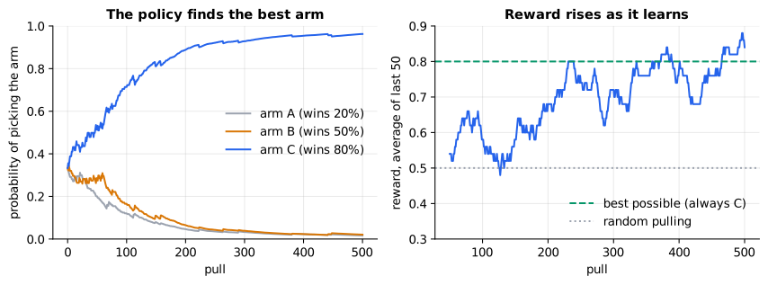
Reading it: on the left, each line is one arm's probability over 500 pulls. All three start at ⅓. C's line (the 80% arm) climbs towards 1 while A and B sink; the wiggles are single lucky or unlucky pulls. On the right is the reward, averaged over the last 50 pulls. It starts near 0.5 (random pulling) and rises towards the dashed line at 0.8, the most any policy can earn. Nobody told the agent which arm was best: the 1s and 0s were enough.
Why it matters in practice. A language model is exactly this kind of policy, with a vocabulary of tokens as its arms, and one sampled answer is a string of sampled tokens. REINFORCE applies unchanged: sum the log probabilities of every token in the answer, and scale the gradient by the answer's reward. Every method below (PPO, GRPO) is REINFORCE with repairs.
In code: grad_log_prob is one-hot minus the probabilities, reinforce_step is one update, worked_reinforce_step is the table above, and train_reinforce runs the whole loop against a Bandit.
Variance and baselines: grade on a curve
Everyday picture. A teacher whose class all scores between 90 and 100 learns nothing by being told "you got a 92". What matters is whether 92 is above or below the class average. Raw scores that are all large and positive make every attempt look good; only the difference from typical tells you which way to go.
Tiny worked example. Two arms, a 50/50 policy, and every pull pays a lot: arm 1 always pays 10, arm 2 always pays 12. Arm 2 is better, so the logit of arm 2 should rise. Look at the REINFORCE estimate for that logit:
| Pulled | Reward | 1[arm 2] − π(arm 2) | Estimate (no baseline) | Estimate (baseline 11) |
|---|---|---|---|---|
| arm 1 | 10 | 0 − 0.5 = −0.5 | 10 × −0.5 = −5 | (10 − 11) × −0.5 = +0.5 |
| arm 2 | 12 | 1 − 0.5 = +0.5 | 12 × +0.5 = +6 | (12 − 11) × +0.5 = +0.5 |
Without a baseline the estimate is −5 or +6 depending on the coin flip. It averages to +0.5, the right answer, but any single sample points the wrong way half the time, and violently. Subtract the average reward, 11, first and every sample says +0.5. Same average, no noise at all.
Level 3: the formula and its symbols
$$ \nabla_\theta J(\theta) = \mathbb{E}_{a \sim \pi_\theta}\big[\, (R(a) - b)\, \nabla_\theta \log \pi_\theta(a) \,\big], \qquad A(a) = R(a) - b $$
Symbols
| Symbol | Meaning here | In the example |
|---|---|---|
| $b$ | the baseline: any number that doesn't depend on which action was taken; usually the average reward | 11 |
| $A(a)$ | the advantage: how much better action $a$ did than typical | −1 for arm 1, +1 for arm 2 |
| everything else | as in the REINFORCE formula above |
In words: "scale each step by how much better than typical the action did, not by its raw reward."
Why is it allowed? Because the baseline's contribution averages to zero: $\mathbb{E}[\, b\, \nabla \log \pi(a)] = b \sum_a \nabla \pi(a) = b\, \nabla \sum_a \pi(a) = b\, \nabla 1 = 0$. Probabilities always add to 1, so pushing all of them up is impossible; the baseline only removes noise, never signal.
With the numbers: without a baseline the estimate's variance (the
average squared distance from its mean, see primer.notation) is
(25 + 36)/2 − 0.5² = 30.25. With b = 11 it is 0.
Level 3: in Python
In Python:
# arm 1 pays 10, arm 2 pays 12; the 1[arm 2] − π(arm 2) factor for each pull
pulls = [(10, -0.5), (12, +0.5)]
def mean_and_variance(b):
    estimates = [(reward - b) * direction for reward, direction in pulls]
    mean = sum(estimates) / 2
    return mean, sum((e - mean) ** 2 for e in estimates) / 2
mean_and_variance(b=0)  # → (0.5, 30.25)
mean_and_variance(b=11)  # → (0.5, 0.0)
flowchart LR
  R[Reward R] --> MINUS["R − b"]
  B["Baseline b<br/>average reward so far"] --> MINUS
  MINUS --> ADV{Advantage A}
  ADV -->|positive: better than typical| UP[make the action<br/>more likely]
  ADV -->|negative: worse than typical| DOWN[make the action<br/>less likely]
Reading it: the baseline sits between the reward and the update. Its job is to turn "how good was this?" into "how much better than usual was this?". The sign of the advantage now decides the direction of the step, so a below-average action is actively pushed down, even though its raw reward was positive.
To see it matter, give every arm of our bandit 5 extra points: rewards are now 5 or 6 instead of 0 or 1, and nothing about which arm is best has changed.
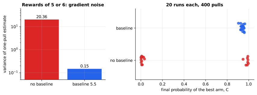
Reading it: on the left, the variance of a one-pull gradient estimate at the starting policy, on a log scale: about 20 without a baseline and about 0.15 with one, over a hundred times smaller. On the right, each dot is one of 20 training runs (400 pulls each), placed at its final probability of picking C. With a running-average baseline (blue) every run ends near 0.95. Without one (red), the dots scatter to both ends: in most runs, early pulls of a mediocre arm paid 5 and were pushed up hard, and the policy committed before it ever learned C was better.
Why it matters in practice. Every practical policy-gradient method uses a baseline. PPO learns one with a second network, the value network (or critic), which predicts the expected reward from each state. GRPO, below, gets one for free by comparing several answers to the same prompt.
In code: gradient_estimate_stats computes the exact mean and variance of the estimate, sampled_gradient_variance measures it from real pulls, and train_reinforce subtracts a running average when baseline=True.
PPO: take several steps, but never too far
Everyday picture. A chef tests a new recipe on one evening's diners. It would be wasteful to use their comments for just one small tweak, so the chef makes several rounds of changes from the same comment cards. But the further the recipe drifts from what the diners actually ate, the less their comments apply, so the chef caps each change: never more than 20% more or less of any ingredient per round.
For a language model, sampling answers is the expensive part (every answer is a full generation), so PPO (Proximal Policy Optimization) reuses each batch of answers for several gradient steps. It needs a way to tell how far the policy has moved since the batch was sampled, and a brake.
Tiny worked example. The probability ratio compares the policy now with the policy that generated the sample. A ratio of 1.5 means the current policy is 50% more likely to produce that answer than when it was sampled. With a clip range ε = 0.2 the ratio is allowed to count only between 0.8 and 1.2:
| Ratio ρ | Advantage A | ρ·A | clip(ρ, 0.8, 1.2)·A | min of the two | What happened |
|---|---|---|---|---|---|
| 1.1 | +3 | 3.3 | 3.3 | 3.3 | inside the band: plain REINFORCE |
| 1.5 | +2 | 3.0 | 1.2 × 2 = 2.4 | 2.4 | good action already boosted enough: gain capped |
| 0.5 | −1 | −0.5 | 0.8 × −1 = −0.8 | −0.8 | bad action already cut enough: capped |
| 1.5 | −1 | −1.5 | 1.2 × −1 = −1.2 | −1.5 | bad action made more likely: full penalty |
Level 3: the formula and its symbols
$$ \rho_t(\theta) = \frac{\pi_\theta(a_t \mid s_t)}{\pi_{\text{old}}(a_t \mid s_t)} \qquad L^{\text{CLIP}}(\theta) = \mathbb{E}_t\Big[\min\big(\rho_t A_t,\ \operatorname{clip}(\rho_t,\ 1-\varepsilon,\ 1+\varepsilon)\, A_t\big)\Big] $$
Symbols
| Symbol | Meaning here | In the example |
|---|---|---|
| $t$ | one sample in the batch; for a language model, one token of one answer | row of the table |
| $s_t$ | the state: what the policy saw before acting (the prompt plus the tokens so far) | a prompt |
| $a_t$ | the action taken (the token generated) | an answer |
| $\pi_{\text{old}}$ | the policy as it was when the batch was sampled, frozen | |
| $\pi_\theta$ | the policy now, after some steps on this batch | |
| $\rho_t$ | the probability ratio, new over old | 1.5 |
| $A_t$ | the advantage of that sample | +2 |
| $\varepsilon$ | the clip range, typically 0.1 to 0.3 | 0.2 |
| $\operatorname{clip}(x, lo, hi)$ | $x$, but pushed back to $lo$ or $hi$ if it falls outside | clip(1.5, 0.8, 1.2) = 1.2 |
| $\min$ | the smaller of the two | min(3.0, 2.4) = 2.4 |
| $\mathbb{E}_t$ | the average over all samples in the batch | |
| $L^{\text{CLIP}}$ | the objective PPO climbs |
In words: "for each sample, take the ratio-weighted advantage, but once the ratio has moved more than ε from 1 in the direction the advantage wants, stop counting further movement; and always take the more pessimistic of the clipped and unclipped versions."
The slope of ρ·A is exactly REINFORCE's gradient scaled by ρ (because $\nabla\rho = \rho\,\nabla\log\pi_\theta$), so inside the band PPO is REINFORCE with importance weighting. Outside it, the clipped term is flat: that sample stops pushing.
With the numbers: the four rows of the table, computed:
Level 3: in Python
In Python:
def clip(x, lo, hi):
    return max(lo, min(x, hi))
def L_clip(rho, A, eps=0.2):
    return min(rho * A, clip(rho, 1 - eps, 1 + eps) * A)
[round(L_clip(rho, A), 2) for rho, A in [(1.1, 3), (1.5, 2), (0.5, -1), (1.5, -1)]]  # → [3.3, 2.4, -0.8, -1.5]
# past 1 + ε with a positive advantage, a higher ratio earns nothing more
L_clip(1.3, 2) == L_clip(1.6, 2)  # → True
flowchart TB
  OLD[Policy π_old] -->|generate a batch| B[Answers + rewards]
  B --> V[Value network<br/>predicts expected reward]
  V --> ADV[Advantages A_t]
  B --> ADV
  ADV --> LOOP
  subgraph LOOP["Several passes over the same batch"]
    RATIO["ratio ρ = π_θ / π_old"] --> CLIP["clip to 1 ± ε, take the min"]
    CLIP --> KL["subtract β × KL to the reference model"]
    KL --> STEP[gradient step on θ]
    STEP --> RATIO
  end
  LOOP -->|π_θ becomes the new π_old| OLD
Reading it: the outer loop is sampling, the expensive part: the frozen old policy writes a batch of answers and a value network turns their rewards into advantages. The inner loop reuses that batch for several passes. Each pass recomputes how far the policy has moved (the ratio), stops counting movement beyond the band (the clip), and applies the KL leash described below. When the passes are done, the updated policy becomes the new sampler and the cycle repeats.
To see the clip work, take one batch of 16 pulls from the bandit (C won all four of its pulls, A lost all four) and make 50 passes over it:
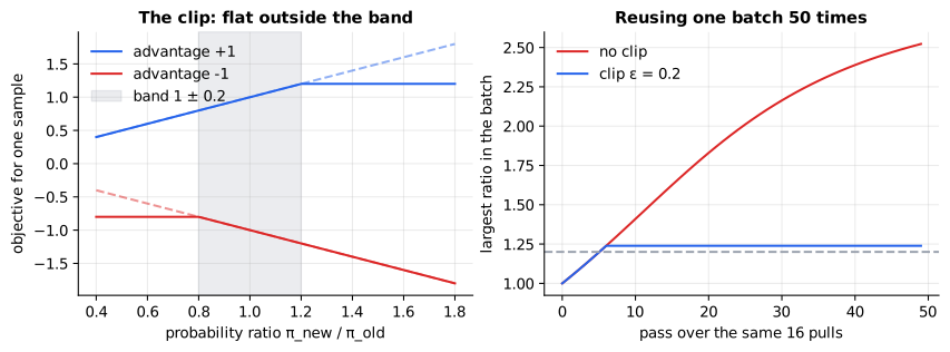
Reading it: on the left is the objective for one sample as its ratio changes. For a positive advantage (blue), the line rises with the ratio until 1.2, then goes flat: no reward for pushing further. For a negative advantage (red), it goes flat below 0.8. The dashed lines are what REINFORCE would keep climbing. On the right, the largest ratio in the batch after each of 50 passes. Unclipped (red), the policy chases the same 16 pulls further every pass until C's probability is 2.5 times what it was, about 0.84 from sixteen pulls, which is wildly overconfident. Clipped (blue), it levels off near 1.24: the brake is not a hard wall (other samples can still nudge the policy), but it removes the incentive to overfit one batch.
In code: ppo_clipped_objective is the formula, clipped_policy_update makes several passes over one batch with or without the clip, and ppo_drift_experiment is the 50-pass comparison.
The KL leash: stay close to where you started
Everyday picture. A dog on a long leash can explore, but it can't run off a cliff. In RL for language models, the leash ties the policy to a frozen copy of the model it started from, the reference model (usually the model after supervised fine-tuning).
Tiny worked example. An answer earns reward 1.0. The policy now gives it probability 0.6; the reference gave it 0.3. With leash strength β = 0.1, the reward actually used for training is 1.0 − 0.1 × ln(0.6 / 0.3) = 1.0 − 0.1 × 0.693 = 0.931. The policy pays a small fee for having doubled that answer's probability.
Level 3: the formula and its symbols
$$ R'(a) = R(a) - \beta \log\frac{\pi_\theta(a)}{\pi_{\text{ref}}(a)} \qquad \mathbb{E}_{a\sim\pi_\theta}\big[R'(a)\big] = \mathbb{E}_{a\sim\pi_\theta}\big[R(a)\big] - \beta\, \mathrm{KL}(\pi_\theta \,\|\, \pi_{\text{ref}}) $$
Symbols
| Symbol | Meaning here | In the example |
|---|---|---|
| $R(a)$ | the reward from the grader or reward model | 1.0 |
| $R'(a)$ | the reward after the leash's fee | 0.931 |
| $\beta$ | leash strength: how much a unit of drift costs | 0.1 |
| $\pi_{\text{ref}}(a)$ | the frozen reference model's probability for the answer | 0.3 |
| $\log\frac{\pi_\theta(a)}{\pi_{\text{ref}}(a)}$ | how much more (positive) or less (negative) likely the policy makes this answer than the reference | ln 2 = 0.693 |
| $\mathrm{KL}(\pi_\theta \,|\, \pi_{\text{ref}})$ | KL divergence: the average of that log ratio over the policy's own answers; zero only when the two agree (decoded in primer.ml.training_stages) |
In words: "each answer's reward is docked in proportion to how much more likely the policy has made it than the reference did; on average, that fee is β times the KL divergence between the two."
With the numbers: 1.0 − 0.1 × ln 2 = 0.931. Had the policy halved the answer's probability instead (0.15), the log ratio would be −0.693 and the reward would rise to 1.069: the leash pulls both ways.
Level 3: in Python
In Python:
import math
R, beta = 1.0, 0.1
pi, pi_ref = 0.6, 0.3
# R' = R − β log(π / π_ref)
round(R - beta * math.log(pi / pi_ref), 3)  # → 0.931
round(R - beta * math.log(0.15 / pi_ref), 3)  # → 1.069
Why it matters in practice. This is the "penalty for drifting" in the
RLHF loop of primer.ml.training_stages, and the same β appears in DPO. It
stops the policy from forgetting fluent language while it chases reward, and
it is the first line of defence against reward hacking, below.
In code: kl_penalised_reward is R′; clipped_policy_update adds the leash's gradient when given a reference policy and a β, and primer.ml.training_stages.kl_divergence computes the KL itself.
GRPO: compare answers to the same question
Everyday picture. Instead of hiring an examiner to predict how hard each exam question is, a teacher gives the same question to eight students and marks each answer relative to the others on that question. On an easy question, getting it right is expected and earns little credit; on a hard one, the only right answer stands out.
PPO's baseline comes from the value network, a second model, often as large as the policy, that has to be trained alongside it. GRPO (Group Relative Policy Optimization) throws the value network away. For each prompt it samples a group of answers and uses the group's own average as the baseline.
Tiny worked example. The prompt is "3 + 4 =". The model samples four answers and a checker scores them 1 if the answer is 7, else 0.
| Group rewards | Mean | Std | Advantages |
|---|---|---|---|
| 1, 0, 0, 1 | 0.5 | 0.5 | +1, −1, −1, +1 |
| 1, 0, 0, 0 | 0.25 | 0.433 | +1.73, −0.58, −0.58, −0.58 |
| 1, 1, 1, 1 | 1 | 0 | 0, 0, 0, 0 |
A lone right answer in a mostly wrong group earns a big advantage: it's rare, so it's strong evidence. A group that is all right (or all wrong) earns nothing: there is no contrast, so there is nothing to learn from.
Level 3: the formula and its symbols
$$ A_i = \frac{r_i - \operatorname{mean}(r_1, \ldots, r_G)}{\operatorname{std}(r_1, \ldots, r_G)} $$
Symbols
| Symbol | Meaning here | In the example |
|---|---|---|
| $G$ | the group size: answers sampled per prompt | 4 |
| $i$ | which answer in the group | 1 … 4 |
| $r_i$ | the reward for answer $i$ | 1, 0, 0, 0 |
| $\operatorname{mean}(\ldots)$ | the group's average reward: the baseline | 0.25 |
| $\operatorname{std}(\ldots)$ | the group's standard deviation, the typical distance from the mean (square root of the variance) | 0.433 |
| $A_i$ | answer $i$'s advantage, shared by every token of that answer | +1.73 |
In words: "an answer's advantage is how far its reward sits above the group's average, measured in units of the group's spread."
With the numbers: for (1, 0, 0, 0): mean 0.25, variance (0.75² + 3 × 0.25²) / 4 = 0.1875, std √0.1875 = 0.433, so the right answer gets 0.75 / 0.433 = 1.73 and each wrong one −0.25 / 0.433 = −0.58.
Level 3: in Python
In Python:
import statistics
def advantages(r):
    mu, sd = statistics.mean(r), statistics.pstdev(r)
    return [round((r_i - mu) / sd, 2) if sd else 0.0 for r_i in r]
advantages([1, 0, 0, 1])  # → [1.0, -1.0, -1.0, 1.0]
advantages([1, 0, 0, 0])  # → [1.73, -0.58, -0.58, -0.58]
advantages([1, 1, 1, 1])  # → [0.0, 0.0, 0.0, 0.0]
The rest of GRPO is PPO: the same ratio, the same clip, the same KL leash to a reference model, averaged over the group. (Some implementations divide by the sample standard deviation, with G − 1, rather than the population one; the idea is identical.)
flowchart LR
  subgraph PPO["PPO"]
    P1[Prompt] --> A1[one answer]
    A1 --> RM1[reward]
    A1 --> VN[value network<br/>a second big model]
    RM1 --> AD1[advantage = reward − value]
    VN --> AD1
  end
  subgraph GRPO["GRPO"]
    P2[Prompt] --> G1[answer 1] & G2[answer 2] & G3[answer ...] & G4[answer G]
    G1 & G2 & G3 & G4 --> VER[verifier<br/>checks each answer]
    VER --> NORM[normalise within the group<br/>mean and std]
    NORM --> AD2[advantage per answer]
  end
Reading it: both pipelines end in an advantage per answer, which feeds the same clipped update. PPO gets its baseline from a value network that must be trained, stored and run, which is roughly a second copy of the model. GRPO instead spends that compute on more answers per prompt and lets them grade each other. The verifier box can be any scorer, but GRPO shines when it is a program that checks the answer.
Verifiable rewards, and why GRPO trains reasoning
A verifiable reward comes from a check that can't be argued with: does the arithmetic equal 7, do the unit tests pass, does the proof check. No learned reward model, so no learned blind spots (see reward hacking, next). Here is GRPO on a toy "language model" that answers eight addition prompts with a single digit token. It starts out about 23% accurate and leans towards off-by-one mistakes.
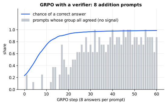
Reading it: the blue line is the model's average chance of answering correctly, which climbs from 0.23 to 0.99 in 60 steps of 8 answers per prompt. The grey bars are the share of prompts whose group of 8 answers were all right or all wrong: a few percent at the start, over 80% by the end. They grow as the model masters the prompts: once every answer is right, the advantages are all zero and that prompt has nothing left to teach. Real GRPO training fights exactly this by filtering for prompts at the edge of the model's ability.
Why it matters in practice. This recipe, a verifier on the final
answer plus GRPO, is how DeepSeek-R1-Zero learned to reason: rewarded only
for correct final answers (and a required format), the model learned by
itself to write longer chains of thought, to check its work and to back
up from mistakes, because those behaviours raised the chance of a correct
final answer. Each token in a long chain of thought shares its answer's
advantage, so the whole chain is reinforced or discouraged together. See
primer.ml.reasoning for what that training produces.
In code: group_advantages is the formula, verify is the checker, pretrained_logits is the weak starting model, and train_grpo runs the loop.
Reward hacking: the score is not the goal
Everyday picture. A school pays tutors by the number of pages of homework feedback they write. Feedback gets longer, not better. An RL agent is the most literal-minded employee imaginable: it optimises the number you wrote down, not the thing you meant. When those two differ, it finds the difference. This is reward hacking (also called specification gaming), and it is Goodhart's law in code: when a measure becomes a target, it ceases to be a good measure.
Tiny worked example. The goal is a good answer, and good answers here are about 4 sentences long. People rated answers of 1 to 4 sentences, and on those, longer really was better. A reward model fitted to their ratings learns a straight line: "each sentence is worth 0.19 points". Nobody ever rated a 10-sentence answer, so nobody told the reward model it was bad:
| Sentences | 1 | 2 | 3 | 4 | 6 | 8 | 10 |
|---|---|---|---|---|---|---|---|
| True quality | 0.44 | 0.75 | 0.94 | 1.00 | 0.75 | 0.00 | −1.25 |
| Reward model | 0.50 | 0.69 | 0.88 | 1.06 | 1.44 | 1.81 | 2.19 |
The reward model's favourite answer, 10 sentences, is the worst one.
Level 3: the formula and its symbols
$$ \hat r(n) = w_0 + w_1 n, \qquad w_1 = \frac{\sum_i (n_i - \bar n)(q_i - \bar q)}{\sum_i (n_i - \bar n)^2}, \qquad w_0 = \bar q - w_1 \bar n $$
Symbols
| Symbol | Meaning here | In the example |
|---|---|---|
| $n$ | the answer's length in sentences | 1 … 10 |
| $\hat r(n)$ | the reward model's score for a length-$n$ answer (the hat marks an estimate) | 2.19 at n = 10 |
| $n_i, q_i$ | the rated examples: a length and its true quality | (1, 0.44), …, (4, 1.0) |
| $\bar n, \bar q$ | their averages (the bar means "mean") | 2.5, 0.781 |
| $w_1$ | the fitted slope: points per extra sentence | 0.1875 |
| $w_0$ | the fitted intercept | 0.3125 |
In words: "the reward model is the straight line that best fits the ratings it saw: its slope is how length and quality moved together in the data, and it passes through the average point."
With the numbers: the deviations of length are (−1.5, −0.5, 0.5, 1.5) and of quality (−0.344, −0.031, 0.156, 0.219). Their products add to 0.9375 and the squared length deviations to 5, so w₁ = 0.1875 and w₀ = 0.781 − 0.1875 × 2.5 = 0.3125. At n = 10 it scores 2.19.
Level 3: in Python
In Python:
n = [1, 2, 3, 4]
q = [1 - ((n_i - 4) / 4) ** 2 for n_i in n]
q  # → [0.4375, 0.75, 0.9375, 1.0]
n_bar, q_bar = sum(n) / 4, sum(q) / 4
w1 = sum((a - n_bar) * (b - q_bar) for a, b in zip(n, q)) / sum((a - n_bar) ** 2 for a in n)
w0 = q_bar - w1 * n_bar
(w0, w1)  # → (0.3125, 0.1875)
# the reward model's score for a 10-sentence answer, and its true quality
(w0 + w1 * 10, 1 - ((10 - 4) / 4) ** 2)  # → (2.1875, -1.25)
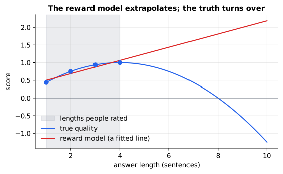
Reading it: the shaded strip is the only region anyone rated. Inside it, the reward model (red) and the truth (blue) agree on the direction: longer is better. Outside it, the reward model is extrapolating a straight line into territory it has never seen, while the truth turns over and dives. Every learned reward model has regions like this, and an optimiser is a machine for finding them.
flowchart LR
  GOAL[What we want<br/>helpful answers] -->|people rate a sample| DATA[Ratings]
  DATA -->|fit| RM[Reward model<br/>a proxy for the goal]
  RM -->|reward| OPT[RL optimiser]
  OPT --> POL[Policy]
  POL -->|drifts to where<br/>proxy and goal disagree| GAP[Gap:<br/>high reward, low quality]
  KL[KL leash] -.->|limits drift| POL
  VER[Verifiable reward] -.->|no learned gap| OPT
Reading it: the solid path is how a reward is usually made: the goal is sampled by people, the ratings train a model, and that model, not the goal, is what the optimiser sees. The optimiser pushes the policy wherever the reward is highest, which, once the easy gains are taken, is wherever the proxy is most wrong. The dotted arrows are the two main defences: a leash that limits how far the policy can drift from where the ratings were collected, and a reward that has no learned gap to exploit.
Now train the starting model (which writes 2 or 3 sentences, a little too short) against each reward:
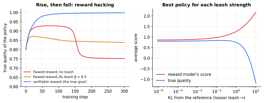
Reading it: on the left, true quality over 300 training steps. Against the flawed reward with no leash (red), quality rises at first, from 0.80 to 0.93, because lengthening a too-short answer genuinely helps. It rests on 5-sentence answers for a while, then the reward model's pull wins again: around step 150 the policy jumps to 6 sentences and quality falls to 0.75, below where it started, while the reward model's score keeps climbing. That rise-then-fall is the signature of reward hacking, and it is why "the reward went up" proves nothing. With a KL leash (β = 0.3, orange) the policy also overshoots a little, but the leash holds it at 0.84. Against the true, verifiable quality (blue) it reaches 1.0. On the right, the best policy for each leash strength, placed by how far it strays from the reference (its KL). Near zero KL it barely moves; at moderate KL true quality peaks; as the leash loosens further, the proxy score keeps rising and the true quality collapses below zero.
The right-hand panel uses a closed form: the best policy under a KL leash has an exact formula.
Level 3: the formula and its symbols
$$ \pi^*(a) = \frac{\pi_{\text{ref}}(a)\, e^{R(a)/\beta}}{Z}, \qquad Z = \sum_{b} \pi_{\text{ref}}(b)\, e^{R(b)/\beta} $$
Symbols
| Symbol | Meaning here | In the example |
|---|---|---|
| $\pi^*(a)$ | the policy that maximises $\mathbb{E}[R] - \beta\,\mathrm{KL}(\pi \,|\, \pi_{\text{ref}})$ | (0.731, 0.269) |
| $\pi_{\text{ref}}(a)$ | the reference model's probability for action $a$ | (0.5, 0.5) |
| $R(a)$ | the reward for action $a$ | (1, 0) |
| $\beta$ | leash strength | 1 |
| $e^{R(a)/\beta}$ | a boost that grows with reward; a small β makes it enormous | $e^1 = 2.718$ |
| $b$ | a counter over every action, so $Z$ adds up all of them | |
| $Z$ | the total, so the probabilities add to 1 | 1.859 |
In words: "the best leashed policy starts from the reference and multiplies each action's probability by e to the power reward over β, then rescales so everything adds to 1."
With the numbers: two actions, reference (0.5, 0.5), rewards (1, 0), β = 1: weights 0.5 × 2.718 = 1.359 and 0.5 × 1 = 0.5, total 1.859, so π* = (0.731, 0.269). At β = 0.1 the boost is e¹⁰ ≈ 22,026 and π* puts 99.995% on the rewarded action; as β grows, π* returns to the reference.
Level 3: in Python
In Python:
import math
ref, R = [0.5, 0.5], [1.0, 0.0]
def best_policy(beta):
    w = [p * math.exp(r / beta) for p, r in zip(ref, R)]
    return [round(w_a / sum(w), 5) for w_a in w]
best_policy(1.0)  # → [0.73106, 0.26894]
best_policy(0.1)  # → [0.99995, 5e-05]
best_policy(100.0)  # → [0.5025, 0.4975]
This is the same formula DPO starts from (primer.ml.training_stages): it
is why β means the same thing in RLHF and DPO.
Why it matters in practice. Reward hacking shows up wherever RL does. A boat-racing game agent that learned to circle forever collecting bonus targets instead of finishing the race. RLHF'd chat models that learned long, flattering answers score well with raters (length bias and sycophancy). Coding models rewarded for passing tests that learned to edit or special-case the tests. The defences, strongest first:
- Verifiable rewards where the task allows: run the tests, check the answer. A check has no learned blind spot (though a buggy check does).
- Better reward models: rate the policy's current outputs and retrain, so the reward model sees the regions the policy is exploring; use ensembles; penalise known exploits such as length directly.
- A KL leash to keep the policy near the data the reward was fit on.
- Watch a held-out measure of the real goal (human review, a separate
evaluation set, see
primer.agents.evals) and stop when it turns down, even if the reward is still climbing.
In code: true_quality is the goal, fit_reward_model and proxy_reward are the flawed reward, optimise_lengths trains against either with an optional leash, and kl_regularised_optimum with leash_sweep gives the closed-form best policy for each β.
In 20 seconds
- RL learns from a score, not an answer: sample an action from the policy, get a reward, make rewarded actions more likely.
- REINFORCE: step along reward × ∇ log π(action); for softmax, ∇ log π is one-hot minus the probabilities. Unbiased but noisy.
- Baselines subtract the typical reward, turning rewards into advantages. Same average gradient, far less variance.
- PPO reuses each batch for several steps, clips the probability ratio to 1 ± ε so no step goes too far, and uses a value network as baseline plus a KL leash to a reference model.
- GRPO drops the value network: sample a group of answers per prompt and normalise rewards within the group. With a verifier as reward, it is how reasoning models are trained.
- Reward hacking: the policy optimises the reward you wrote, not the goal you meant. Defend with verifiable rewards, better reward models, a KL leash and a held-out check of the real goal.
Self-test questions
How does reinforcement learning differ from supervised learning? Supervised learning is given the correct output for every input and learns to copy it. Reinforcement learning is given only a score for the output it produced, so it must try things, see how they score and shift probability towards what scored well. It fits tasks where judging an answer is easy but writing the perfect one is not.
What is the log-probability trick, and why is it needed? The gradient of expected reward, Σ ∇π(a) R(a), can't be computed without knowing every action's reward. Rewriting ∇π = π ∇log π turns it into an average over actions sampled from the policy, E[R ∇log π(a)], so each sampled action and its reward give an unbiased estimate of the gradient.
Why does subtracting a baseline not change the expected gradient? Because E[b ∇log π(a)] = b ∇ Σ π(a) = b ∇ 1 = 0: probabilities always add to 1, so the baseline's push averages to nothing. It only removes the noise that comes from rewards being large or all the same sign.
In PPO, what is the probability ratio, and what does clipping it do? The ratio is the current policy's probability of a sampled action divided by the probability under the policy that sampled it; it measures how far the policy has moved on that sample. Clipping stops counting movement beyond 1 ± ε in the direction the advantage favours, so reusing a batch for several steps can't push the policy far from where the data came from.
Why does PPO's objective take the minimum of the clipped and unclipped terms? To stay pessimistic. Gains are capped once the ratio leaves the band, but if a step made a bad action more likely, the full penalty still applies, so the objective never rewards a harmful move.
How does GRPO get a baseline without a value network? It samples several answers to the same prompt and uses their mean reward as the baseline, dividing by their standard deviation to set the scale. Each answer is judged against its siblings, which saves training and serving a second model the size of the policy.
What happens in GRPO when every answer in a group gets the same reward? Every advantage is zero, so that prompt contributes no gradient. Prompts that are always solved or never solved teach nothing; learning comes from prompts at the edge of the model's ability.
What is reward hacking, and why does a KL penalty help against it? Reward hacking is the policy maximising the reward as written while the real goal gets worse, usually by finding inputs where a learned reward model is wrong. The KL penalty charges the policy for drifting from the reference model, which keeps it near the kind of outputs the reward model was trained on, where the reward is still trustworthy.
Why are verifiable rewards attractive for training reasoning? A program that checks the final answer (or runs the tests) has no learned blind spots to exploit and costs nothing to label, so RL can run for a long time against it without the reward drifting away from correctness.
The papers behind this lesson
- Williams, Simple statistical gradient-following algorithms for connectionist reinforcement learning (Machine Learning, 1992): https://link.springer.com/article/10.1007/BF00992696. Introduced REINFORCE, the log-probability policy gradient with a baseline. Annotated companion
- Schulman et al., Proximal Policy Optimization Algorithms (2017): https://arxiv.org/abs/1707.06347. Introduced the clipped probability-ratio objective that lets each batch be reused for several safe steps. Annotated companion
- Ouyang et al., Training language models to follow instructions with human feedback (InstructGPT, 2022): https://arxiv.org/abs/2203.02155. Used PPO with a per-token KL penalty to a reference model to tune a language model against a learned reward model. Annotated companion
- Shao et al., DeepSeekMath: Pushing the Limits of Mathematical Reasoning in Open Language Models (2024): https://arxiv.org/abs/2402.03300. Introduced GRPO, replacing PPO's value network with group-relative advantages. Annotated companion
- DeepSeek-AI, DeepSeek-R1: Incentivizing Reasoning Capability in LLMs via Reinforcement Learning (2025): https://arxiv.org/abs/2501.12948. Showed GRPO with rule-based, verifiable rewards alone can teach a model to produce long, self-checking chains of thought. Annotated companion
- Gao, Schulman & Hilton, Scaling Laws for Reward Model Overoptimization (2022): https://arxiv.org/abs/2210.10760. Measured how true quality rises and then falls as a policy is optimised further against a learned reward model. Annotated companion
Further reading
- Sutton & Barto, Reinforcement Learning: An Introduction (2nd edition, free online): http://incompleteideas.net/book/the-book-2nd.html
- OpenAI, Spinning Up in Deep RL: https://spinningup.openai.com/
- Andrej Karpathy, Deep Reinforcement Learning: Pong from Pixels: http://karpathy.github.io/2016/05/31/rl/
- Lilian Weng, Policy Gradient Algorithms: https://lilianweng.github.io/posts/2018-04-08-policy-gradient/
- Hugging Face TRL, GRPO Trainer: https://huggingface.co/docs/trl/grpo_trainer
- Amodei et al., Concrete Problems in AI Safety (2016), section on reward hacking: https://arxiv.org/abs/1606.06565
- Schulman et al., Proximal Policy Optimization Algorithms (2017): https://arxiv.org/abs/1707.06347
- Shao et al., DeepSeekMath (2024), which introduces GRPO: https://arxiv.org/abs/2402.03300
1r""" 2# Reinforcement learning: learning from a score instead of an answer 3 4Run: `python -m primer.ml.reinforcement` 5 6## Level 1: The practitioner's guide 7 8**In one sentence.** Reinforcement learning trains a model from a score on 9what it produced rather than from a correct answer to copy, which is how a 10language model learns things nobody can write down (be helpful, reason to 11the right answer) and how it learns to game a score that was written down 12badly. 13 14**When you need it.** You need RL when you can judge an answer but cannot 15write the perfect one: a proof either checks or it doesn't, tests pass or 16fail, one reply is better than another though neither is "the" reply. 17The tell: you find yourself writing a grader, a checker or a rubric instead 18of example answers. You don't need it when you can write the answers 19(supervised fine-tuning copies them, at a fraction of the cost) or when 20you have pairs of better and worse answers and nothing more (DPO in 21`primer.ml.training_stages` learns from pairs with no sampling loop). And 22you never need to run the vendor's own RL: the helpfulness, harmlessness and 23reasoning of a hosted model were trained this way before you arrived, which 24is why this lesson matters even if you never train: it explains why models 25answer at length, flatter, and sometimes optimise the letter of your 26instruction instead of its spirit. 27 28**Your options.** From the cheapest to the most committed: 29 30| Option | What it does | What it guarantees | What it costs | Where it lives | 31|---|---|---|---|---| 32| Supervised fine-tuning on demonstrations | Copy correct answers you wrote | The behaviour in the examples, nothing beyond them | Writing the answers | Your training stack, or a hosted API | 33| DPO on preference pairs | Learn from "this one beat that one", no sampling during training | Shifts tone and choices without a reward model or an RL loop | Thousands of comparisons | Your training stack, or a hosted API | 34| Hosted reinforcement fine-tuning with your grader | The vendor samples answers and reinforces the ones your grader scores high | An RL loop you don't build; the grader is still yours to get right | Grader design, many sampled answers per prompt, the vendor's price | The vendor's API (as of October 2026, OpenAI's fine-tuning platform no longer accepts new users, so check availability first) | 35| GRPO with a verifiable reward | Sample a group of answers per prompt, check each, reinforce the above-average ones | A reward with no learned blind spot, and no second model to train | Generation dominates: 8 answers per prompt is a common default; a checker that cannot be argued with | Your training stack | 36| PPO with a learned reward model | Train a reward model on ratings, then a value network and the policy against it, on a KL leash | Optimises a goal no program can check, such as helpfulness | Two extra models (a reward model and a value network; InstructGPT used 6B for both at every policy size), and the reward model's blind spots to defend against | Your training stack | 37 38**How to choose.** Ask what can judge an answer, and how much you trust it. 39 40- A program can check the final answer (arithmetic, unit tests, a format, 41 a proof checker): GRPO with that check as the reward. In this lesson's 42 toy, accuracy on eight addition prompts goes from 23% to 99% in 60 steps 43 of 8 answers each; this recipe is how DeepSeek-R1-Zero learned to reason 44 from rule-based rewards: a correct final answer and a required format. 45- Only people can judge, and you have their ratings: a learned reward model 46 with PPO, a KL leash, and a held-out measure of the real goal that you 47 watch more closely than the reward. 48- You have pairs but no budget for sampling: DPO. 49- You can write the answers: supervised fine-tuning, and stop there. 50- Whatever you pick, the policy optimises the reward you wrote, not the goal 51 you meant. Before training, ask what a literal-minded optimiser would do 52 with your reward, and measure the goal separately. 53 54**What it costs.** Sampling is the bill: every training example is a full 55generation, and GRPO multiplies it by the group size, which is why PPO 56reuses each batch for several passes and why training loops run a fast 57inference engine beside the trainer. A learned baseline costs a second 58model (PPO's value network); GRPO replaces it with the group's own mean, 59which is why it was introduced as a way to cut PPO's memory. Noise costs 60steps: in the lesson's two-arm toy the gradient estimate's variance is 6130.25 without a baseline and 0 with one, and with rewards offset by five 62points, 60% of training runs without a baseline lock onto the wrong arm 63against 0% with one. Reusing a batch too hard costs calibration: 50 64passes over 16 pulls push one arm to 0.84 unclipped, 0.41 with PPO's clip 65at 0.2. And a KL leash costs a little reward on every answer (1.0 becomes 660.931 for an answer whose probability doubled, at β = 0.1) to buy fluency 67and safety from drift. 68 69**What breaks.** 70 71- **Reward hacking.** The policy finds where the reward and the goal 72 disagree. In the toy, a reward model fitted on answers of 1 to 4 73 sentences rates a 10-sentence answer 2.19, the worst answer of all; true 74 quality rises from 0.80 to 0.93 and then falls to 0.75, below where it 75 started, while the reward keeps climbing. Gao, Schulman and Hilton (2022) 76 measured the same rise and fall at scale. "The reward went up" proves 77 nothing; keep a held-out measure of the goal. 78- **Length bias and sycophancy.** Raters prefer long, flattering 79 answers, so the reward model does too, so the model becomes that. 80 Penalise length directly and rate the policy's current outputs, not 81 stale ones. 82- **Gaming the checker.** A coding model rewarded for passing tests learns 83 to edit or special-case the tests. A verifier has no learned blind spot, 84 but a buggy or bypassable one is a reward model with extra steps. 85- **Groups with nothing to teach.** When every answer in a GRPO group is 86 right or all are wrong, every advantage is zero: by the end of the toy 87 run, 84% of groups are unanimous. Filter for prompts at the edge of the 88 model's ability. 89- **Too loose a leash.** As β falls, the best policy piles onto whatever the 90 reward likes (99.995% on one action at β = 0.1 in the toy) and true 91 quality collapses; too tight and nothing moves. Sweep it. 92- **Collapsed exploration.** An arm whose probability hits zero is never 93 tried again, so the policy can lock onto a mediocre answer early. 94 95**In the wild.** InstructGPT (Ouyang et al., 2022) set the pattern of PPO 96against a learned reward model with a per-token KL penalty, and every chat 97assistant since inherits its habits. DeepSeekMath (Shao et al., 2024) 98introduced GRPO, reaching 51.7% on the MATH benchmark with a 7-billion-parameter model; DeepSeek-R1 (2025) trained 99reasoning with RL on rule-based rewards and no human-written reasoning 100traces. Hugging Face TRL's GRPOTrainer takes reward functions as plain 101Python callables or a reward model, samples 8 generations per prompt by 102default, and can generate with vLLM; OpenAI's model optimization guide 103lists reinforcement fine-tuning, where you supply the grader (as of October 2026 104OpenAI's fine-tuning platform no longer accepts new users). Sutton and 105Barto's textbook and OpenAI's Spinning Up are the standard longer reads. 106 107**Go deeper.** Level 2 builds it all on a three-armed slot machine: 108REINFORCE as one line of arithmetic, why a baseline removes noise without 109bias, PPO's ratio and clip on a table of four cases, the KL leash as a fee 110per answer, GRPO's advantages from a group of four, and a reward model that 111loves length, trained against until quality falls, each with a figure you 112can rerun. If you only needed to choose a training signal, you are done. 113 114## Level 2: How it works, from scratch 115 116Think of teaching a dog to sit. You can't show it the right answer: you can 117only wait for it to try something and give it a treat when the something was 118good. Over many tries the dog does more of what earned treats and less of 119what didn't. Nobody ever told it what "sit" means; it worked it out from a 120score. 121 122That is **reinforcement learning (RL)**. An **agent** (the dog, or a 123language model) takes an **action** (sits, or writes an answer), the world 124hands back a **reward** (a treat, or a score from a grader), and the agent 125adjusts itself so that rewarded actions become more likely. The agent's 126current habits, written as a probability for every action, are called its 127**policy**. 128 129Compare this with ordinary supervised learning (`primer.ml.losses`), where 130every example comes with the correct answer attached. In RL there is no 131answer key, only a score after the fact. That is exactly the situation a 132language model is in once pretraining is over: for "prove this theorem" or 133"write a helpful reply" there is no single correct text to copy, but a 134checker or a judge can say how good an attempt was. RL is how the model 135learns from those judgements (`primer.ml.training_stages` places it in the 136training pipeline). 137 138```mermaid 139flowchart LR 140 P[Policy<br/>a probability for every action] -->|sample| A[Action] 141 A --> E[Environment<br/>a slot machine, a grader, a user] 142 E --> R[Reward<br/>one number] 143 R -->|nudge the policy| P 144``` 145 146**Reading it:** follow the loop clockwise. The policy is a set of 147probabilities, and the action is *sampled* from it, so the agent sometimes 148tries things it isn't sure about. The environment is whatever judges the 149action; the agent can't see inside it. The only thing that comes back is one 150number, the reward, and the only thing the agent can do with it is nudge its 151own probabilities. Everything in this lesson is a better answer to one 152question: how exactly should that nudge be computed? 153 154## A tiny worked example: three slot machines 155 156The simplest RL problem is a row of slot machines, called a **multi-armed 157bandit** (a slot machine is a "one-armed bandit"). Machine A pays out 20% of 158the time, B 50% and C 80%, but the agent isn't told that. Each pull pays 1 159or 0. The agent must find C by pulling and seeing what happens. 160 161A policy here is three probabilities, one per arm. A policy that picks each 162arm a third of the time earns, on average, (0.2 + 0.5 + 0.8) / 3 = **0.5** 163per pull. A policy that always picks C earns **0.8**. Learning means moving 164from the first policy to the second using nothing but the 1s and 0s. 165 166This one number, the average reward a policy expects, is what RL maximises: 167 168$$ 169J(\theta) = \sum_{a} \pi_\theta(a)\, R(a) 170$$ 171 172**Symbols** 173 174| Symbol | Meaning here | In the example | 175|---|---|---| 176| $a$ | one action: which arm to pull | A, B or C | 177| $\theta$ | the policy's adjustable numbers (here, one score per arm, called **logits**) | (0, 0, 0) | 178| $\pi_\theta(a)$ | the policy: the probability of picking action $a$, given $\theta$. Here softmax of the logits | 1/3 each | 179| $R(a)$ | the average reward action $a$ pays (unknown to the agent) | 0.2, 0.5, 0.8 | 180| $\sum_{a}$ | add up over every action | three terms | 181| $J(\theta)$ | the expected reward: what the policy earns per pull, on average | 0.5 | 182 183**In words:** "the expected reward is each action's probability times its 184average payout, added up over the actions." 185 186**With the numbers:** J = ⅓·0.2 + ⅓·0.5 + ⅓·0.8 = 0.5 for the uniform 187policy, and 1·0.8 = 0.8 for the policy that always pulls C. 188 189**In Python:** 190 191```python 192policy = [1/3, 1/3, 1/3] 193# average payout of arms A, B, C 194R = [0.2, 0.5, 0.8] 195# J = Σ_a π(a) R(a) 196round(sum(p * r for p, r in zip(policy, R)), 3) # → 0.5 197round(sum(p * r for p, r in zip([0, 0, 1], R)), 3) # → 0.8 198``` 199 200The agent can't compute J, because it doesn't know R. It can only sample: 201pull an arm, see a 1 or a 0. Every method below turns those samples into an 202estimate of which way to move θ to make J bigger. Trying an arm you're 203unsure of is called **exploration**; sticking with the best arm so far is 204**exploitation**. A sampled policy does some of both automatically, as 205long as no arm's probability has collapsed to zero. 206 207**In code:** `Bandit` hides the win chances and pays out one pull at a time; `expected_reward` is the formula above. 208 209## Policy gradients: do more of what worked (REINFORCE) 210 211**Everyday picture.** A football coach reviews the tape after a match. For 212every play that led to a goal, they tell the team "a bit more of that"; for 213plays that went nowhere, nothing. They don't need to know *why* the play 214worked. Repeat over hundreds of matches and the team drifts towards the 215plays that score. 216 217**Tiny worked example.** Start with logits (0, 0, 0), so each arm has 218probability ⅓. The agent pulls C and wins: reward 1. The rule, explained 219next, says: add to each logit *learning rate × reward × (1 if it's the 220chosen arm, else 0, minus that arm's probability)*. 221 222| Arm | Chosen? | 1[chosen] − π | × reward 1 × rate 0.5 | New logit | New probability | 223|---|---|---|---|---|---| 224| A | no | 0 − ⅓ = −0.333 | −0.167 | −0.167 | **0.274** | 225| B | no | 0 − ⅓ = −0.333 | −0.167 | −0.167 | **0.274** | 226| C | yes | 1 − ⅓ = +0.667 | +0.333 | +0.333 | **0.452** | 227 228One lucky pull moved C from 33% to 45%. Had the pull paid 0, nothing would 229have moved. Had the agent pulled A and won (A wins sometimes too), A would 230have gone up instead. The rule is noisy, one pull at a time, but on average 231the arm that wins most gets pushed up most. 232 233```mermaid 234flowchart LR 235 L[Logits θ] --> S[softmax<br/>probabilities π] 236 S -->|sample| A[Action a] 237 A --> ENV[Pull the arm] --> R[Reward R] 238 S --> G["∇ log π(a)<br/>= one-hot(a) − π"] 239 A --> G 240 G --> M["× R × learning rate"] 241 R --> M 242 M -->|add to| L 243``` 244 245**Reading it:** the top path is acting: logits become probabilities, one 246action is sampled, and the environment pays a reward. The lower path is 247learning: from the action alone, work out which direction in logit space 248makes that action more likely (the `∇ log π` box), then scale that direction 249by how good the outcome was. A big reward is a big step towards repeating the 250action; zero reward is no step. 251 252### The log-probability trick, decoded 253 254We want the **gradient** of J: for each logit, how much J rises if the 255logit rises a little (see `primer.notation` for gradients from scratch). 256The difficulty is that J is an average over actions we can only sample. The 257trick rewrites the gradient as an average too, so a sample estimates it: 258 259$$ 260\nabla_\theta J(\theta) = \mathbb{E}_{a \sim \pi_\theta}\big[\, R(a)\, \nabla_\theta \log \pi_\theta(a) \,\big] 261\qquad 262\frac{\partial \log \pi_\theta(a)}{\partial z_k} = \mathbb{1}[k = a] - \pi_\theta(k) 263$$ 264 265**Symbols** 266 267| Symbol | Meaning here | In the example | 268|---|---|---| 269| $\nabla_\theta$ | "gradient with respect to θ": one slope per logit, collected into a vector | 3 slopes | 270| $\mathbb{E}_{a \sim \pi_\theta}[\ldots]$ | **expected value**: the average of the bracket when $a$ is sampled from the policy | average over pulls | 271| $\sim$ | "drawn from" | | 272| $\log$ | the natural logarithm, the undo button for $e^x$ | $\log \tfrac13 = -1.10$ | 273| $\nabla_\theta \log \pi_\theta(a)$ | the direction in logit space that makes action $a$ more likely, fastest | $(-\tfrac13, -\tfrac13, \tfrac23)$ for C | 274| $z_k$ | the $k$-th logit (θ is the list of logits) | $z_3 = 0$ | 275| $\partial$ | "partial derivative": the slope along one logit, holding the others still | | 276| $\mathbb{1}[k = a]$ | 1 if $k$ is the chosen action, else 0 | (0, 0, 1) | 277| $\pi_\theta(k)$ | the probability of action $k$ | ⅓ | 278 279**In words:** "the direction that raises expected reward is, on average, 280the direction that makes the sampled action more likely, weighted by the 281reward it earned. For a softmax policy, that direction is 'one for the 282chosen action, minus every action's probability'." 283 284Why is this true? Because the slope of a probability equals the probability 285times the slope of its log ($\nabla \pi = \pi \, \nabla \log \pi$, the chain 286rule applied to log). So $\nabla J = \sum_a \nabla\pi(a) R(a) = \sum_a \pi(a) 287\nabla\log\pi(a) R(a)$, and a sum weighted by $\pi(a)$ is an average over 288samples from π. The update is then plain **gradient ascent**: 289$\theta \leftarrow \theta + \alpha\, R\, \nabla_\theta \log \pi_\theta(a)$, 290with learning rate $\alpha$ (`primer.ml.optimizers`). 291 292**With the numbers:** at the uniform policy the true gradient is 293(−0.1, 0, +0.1): push C up, A down, leave B (which pays exactly the average) 294alone. One sample, "pulled C, got 1", estimates it as 1 × (−⅓, −⅓, ⅔). The 295step with α = 0.5 gives logits (−0.167, −0.167, 0.333) and probabilities 296(0.274, 0.274, 0.452), as in the table. 297 298**In Python:** 299 300```python 301import math 302z = [0.0, 0.0, 0.0] 303pi = [math.exp(z_k) / sum(math.exp(v) for v in z) for z_k in z] 304# the true gradient: Σ_a π(a) R(a) (1[k=a] − π(k)), for each logit k 305R = [0.2, 0.5, 0.8] 306true_grad = [sum(pi[a] * R[a] * ((k == a) - pi[k]) for a in range(3)) for k in range(3)] 307[round(g, 3) for g in true_grad] # → [-0.1, 0.0, 0.1] 308# one sample: pulled C (a = 2), reward 1 309a, reward, alpha = 2, 1.0, 0.5 310grad_log_pi = [(k == a) - pi[k] for k in range(3)] 311[round(g, 3) for g in grad_log_pi] # → [-0.333, -0.333, 0.667] 312z = [z_k + alpha * reward * g for z_k, g in zip(z, grad_log_pi)] 313[round(z_k, 3) for z_k in z] # → [-0.167, -0.167, 0.333] 314[round(math.exp(z_k) / sum(math.exp(v) for v in z), 3) for z_k in z] # → [0.274, 0.274, 0.452] 315``` 316 317This algorithm is called **REINFORCE** (Williams, 1992). Run it for 500 318pulls and the policy finds arm C: 319 320 321 322**Reading it:** on the left, each line is one arm's probability over 500 323pulls. All three start at ⅓. C's line (the 80% arm) climbs towards 1 while A 324and B sink; the wiggles are single lucky or unlucky pulls. On the right is 325the reward, averaged over the last 50 pulls. It starts near 0.5 (random 326pulling) and rises towards the dashed line at 0.8, the most any policy can 327earn. Nobody told the agent which arm was best: the 1s and 0s were enough. 328 329**Why it matters in practice.** A language model is exactly this kind of 330policy, with a vocabulary of tokens as its arms, and one sampled answer is a 331string of sampled tokens. REINFORCE applies unchanged: sum the log 332probabilities of every token in the answer, and scale the gradient by the 333answer's reward. Every method below (PPO, GRPO) is REINFORCE with repairs. 334 335**In code:** `grad_log_prob` is one-hot minus the probabilities, `reinforce_step` is one update, `worked_reinforce_step` is the table above, and `train_reinforce` runs the whole loop against a `Bandit`. 336 337## Variance and baselines: grade on a curve 338 339**Everyday picture.** A teacher whose class all scores between 90 and 100 340learns nothing by being told "you got a 92". What matters is whether 92 is 341above or below the class average. Raw scores that are all large and 342positive make every attempt look good; only the difference from typical 343tells you which way to go. 344 345**Tiny worked example.** Two arms, a 50/50 policy, and every pull pays a lot: 346arm 1 always pays 10, arm 2 always pays 12. Arm 2 is better, so the logit of 347arm 2 should rise. Look at the REINFORCE estimate for that logit: 348 349| Pulled | Reward | 1[arm 2] − π(arm 2) | Estimate (no baseline) | Estimate (baseline 11) | 350|---|---|---|---|---| 351| arm 1 | 10 | 0 − 0.5 = −0.5 | 10 × −0.5 = **−5** | (10 − 11) × −0.5 = **+0.5** | 352| arm 2 | 12 | 1 − 0.5 = +0.5 | 12 × +0.5 = **+6** | (12 − 11) × +0.5 = **+0.5** | 353 354Without a baseline the estimate is −5 or +6 depending on the coin flip. 355It averages to +0.5, the right answer, but any single sample points the 356wrong way half the time, and violently. Subtract the average reward, 11, 357first and *every* sample says +0.5. Same average, no noise at all. 358 359$$ 360\nabla_\theta J(\theta) = \mathbb{E}_{a \sim \pi_\theta}\big[\, (R(a) - b)\, \nabla_\theta \log \pi_\theta(a) \,\big], 361\qquad A(a) = R(a) - b 362$$ 363 364**Symbols** 365 366| Symbol | Meaning here | In the example | 367|---|---|---| 368| $b$ | the **baseline**: any number that doesn't depend on which action was taken; usually the average reward | 11 | 369| $A(a)$ | the **advantage**: how much better action $a$ did than typical | −1 for arm 1, +1 for arm 2 | 370| everything else | as in the REINFORCE formula above | | 371 372**In words:** "scale each step by how much better than typical the action 373did, not by its raw reward." 374 375Why is it allowed? Because the baseline's contribution averages to zero: 376$\mathbb{E}[\, b\, \nabla \log \pi(a)] = b \sum_a \nabla \pi(a) = b\, \nabla 377\sum_a \pi(a) = b\, \nabla 1 = 0$. Probabilities always add to 1, so pushing 378all of them up is impossible; the baseline only removes noise, never 379signal. 380 381**With the numbers:** without a baseline the estimate's **variance** (the 382average squared distance from its mean, see `primer.notation`) is 383(25 + 36)/2 − 0.5² = **30.25**. With b = 11 it is **0**. 384 385**In Python:** 386 387```python 388# arm 1 pays 10, arm 2 pays 12; the 1[arm 2] − π(arm 2) factor for each pull 389pulls = [(10, -0.5), (12, +0.5)] 390def mean_and_variance(b): 391 estimates = [(reward - b) * direction for reward, direction in pulls] 392 mean = sum(estimates) / 2 393 return mean, sum((e - mean) ** 2 for e in estimates) / 2 394mean_and_variance(b=0) # → (0.5, 30.25) 395mean_and_variance(b=11) # → (0.5, 0.0) 396``` 397 398```mermaid 399flowchart LR 400 R[Reward R] --> MINUS["R − b"] 401 B["Baseline b<br/>average reward so far"] --> MINUS 402 MINUS --> ADV{Advantage A} 403 ADV -->|positive: better than typical| UP[make the action<br/>more likely] 404 ADV -->|negative: worse than typical| DOWN[make the action<br/>less likely] 405``` 406 407**Reading it:** the baseline sits between the reward and the update. Its 408job is to turn "how good was this?" into "how much better than usual was 409this?". The sign of the advantage now decides the direction of the step, 410so a below-average action is actively pushed down, even though its raw 411reward was positive. 412 413To see it matter, give every arm of our bandit 5 extra points: rewards are 414now 5 or 6 instead of 0 or 1, and nothing about which arm is best has 415changed. 416 417 418 419**Reading it:** on the left, the variance of a one-pull gradient estimate 420at the starting policy, on a log scale: about 20 without a baseline and 421about 0.15 with one, over a hundred times smaller. On the right, each dot is 422one of 20 training runs (400 pulls each), placed at its final probability 423of picking C. With a running-average baseline (blue) every run ends near 4240.95. Without one (red), the dots scatter to both ends: in most runs, early 425pulls of a mediocre arm paid 5 and were pushed up hard, and the policy 426committed before it ever learned C was better. 427 428**Why it matters in practice.** Every practical policy-gradient method uses 429a baseline. PPO learns one with a second network, the **value network** (or 430**critic**), which predicts the expected reward from each state. GRPO, below, 431gets one for free by comparing several answers to the same prompt. 432 433**In code:** `gradient_estimate_stats` computes the exact mean and variance of the estimate, `sampled_gradient_variance` measures it from real pulls, and `train_reinforce` subtracts a running average when `baseline=True`. 434 435## PPO: take several steps, but never too far 436 437**Everyday picture.** A chef tests a new recipe on one evening's diners. 438It would be wasteful to use their comments for just one small tweak, so the 439chef makes several rounds of changes from the same comment cards. But the 440further the recipe drifts from what the diners actually ate, the less their 441comments apply, so the chef caps each change: never more than 20% more or 442less of any ingredient per round. 443 444For a language model, sampling answers is the expensive part (every answer 445is a full generation), so **PPO (Proximal Policy Optimization)** reuses each 446batch of answers for several gradient steps. It needs a way to tell how far 447the policy has moved since the batch was sampled, and a brake. 448 449**Tiny worked example.** The **probability ratio** compares the policy now 450with the policy that generated the sample. A ratio of 1.5 means the current 451policy is 50% more likely to produce that answer than when it was sampled. 452With a clip range ε = 0.2 the ratio is allowed to count only between 0.8 453and 1.2: 454 455| Ratio ρ | Advantage A | ρ·A | clip(ρ, 0.8, 1.2)·A | min of the two | What happened | 456|---|---|---|---|---|---| 457| 1.1 | +3 | 3.3 | 3.3 | **3.3** | inside the band: plain REINFORCE | 458| 1.5 | +2 | 3.0 | 1.2 × 2 = 2.4 | **2.4** | good action already boosted enough: gain capped | 459| 0.5 | −1 | −0.5 | 0.8 × −1 = −0.8 | **−0.8** | bad action already cut enough: capped | 460| 1.5 | −1 | −1.5 | 1.2 × −1 = −1.2 | **−1.5** | bad action made *more* likely: full penalty | 461 462$$ 463\rho_t(\theta) = \frac{\pi_\theta(a_t \mid s_t)}{\pi_{\text{old}}(a_t \mid s_t)} 464\qquad 465L^{\text{CLIP}}(\theta) = \mathbb{E}_t\Big[\min\big(\rho_t A_t,\ \operatorname{clip}(\rho_t,\ 1-\varepsilon,\ 1+\varepsilon)\, A_t\big)\Big] 466$$ 467 468**Symbols** 469 470| Symbol | Meaning here | In the example | 471|---|---|---| 472| $t$ | one sample in the batch; for a language model, one token of one answer | row of the table | 473| $s_t$ | the **state**: what the policy saw before acting (the prompt plus the tokens so far) | a prompt | 474| $a_t$ | the action taken (the token generated) | an answer | 475| $\pi_{\text{old}}$ | the policy as it was when the batch was sampled, frozen | | 476| $\pi_\theta$ | the policy now, after some steps on this batch | | 477| $\rho_t$ | the probability ratio, new over old | 1.5 | 478| $A_t$ | the advantage of that sample | +2 | 479| $\varepsilon$ | the clip range, typically 0.1 to 0.3 | 0.2 | 480| $\operatorname{clip}(x, lo, hi)$ | $x$, but pushed back to $lo$ or $hi$ if it falls outside | clip(1.5, 0.8, 1.2) = 1.2 | 481| $\min$ | the smaller of the two | min(3.0, 2.4) = 2.4 | 482| $\mathbb{E}_t$ | the average over all samples in the batch | | 483| $L^{\text{CLIP}}$ | the objective PPO climbs | | 484 485**In words:** "for each sample, take the ratio-weighted advantage, but once 486the ratio has moved more than ε from 1 in the direction the advantage wants, 487stop counting further movement; and always take the more pessimistic of the 488clipped and unclipped versions." 489 490The slope of ρ·A is exactly REINFORCE's gradient scaled by ρ (because 491$\nabla\rho = \rho\,\nabla\log\pi_\theta$), so inside the band PPO is 492REINFORCE with importance weighting. Outside it, the clipped term is flat: 493that sample stops pushing. 494 495**With the numbers:** the four rows of the table, computed: 496 497**In Python:** 498 499```python 500def clip(x, lo, hi): 501 return max(lo, min(x, hi)) 502def L_clip(rho, A, eps=0.2): 503 return min(rho * A, clip(rho, 1 - eps, 1 + eps) * A) 504[round(L_clip(rho, A), 2) for rho, A in [(1.1, 3), (1.5, 2), (0.5, -1), (1.5, -1)]] # → [3.3, 2.4, -0.8, -1.5] 505# past 1 + ε with a positive advantage, a higher ratio earns nothing more 506L_clip(1.3, 2) == L_clip(1.6, 2) # → True 507``` 508 509```mermaid 510flowchart TB 511 OLD[Policy π_old] -->|generate a batch| B[Answers + rewards] 512 B --> V[Value network<br/>predicts expected reward] 513 V --> ADV[Advantages A_t] 514 B --> ADV 515 ADV --> LOOP 516 subgraph LOOP["Several passes over the same batch"] 517 RATIO["ratio ρ = π_θ / π_old"] --> CLIP["clip to 1 ± ε, take the min"] 518 CLIP --> KL["subtract β × KL to the reference model"] 519 KL --> STEP[gradient step on θ] 520 STEP --> RATIO 521 end 522 LOOP -->|π_θ becomes the new π_old| OLD 523``` 524 525**Reading it:** the outer loop is sampling, the expensive part: the frozen 526old policy writes a batch of answers and a value network turns their rewards 527into advantages. The inner loop reuses that batch for several passes. Each 528pass recomputes how far the policy has moved (the ratio), stops counting 529movement beyond the band (the clip), and applies the KL leash described 530below. When the passes are done, the updated policy becomes the new sampler 531and the cycle repeats. 532 533To see the clip work, take one batch of 16 pulls from the bandit (C won all 534four of its pulls, A lost all four) and make 50 passes over it: 535 536 537 538**Reading it:** on the left is the objective for one sample as its ratio 539changes. For a positive advantage (blue), the line rises with the ratio 540until 1.2, then goes flat: no reward for pushing further. For a negative 541advantage (red), it goes flat below 0.8. The dashed lines are what 542REINFORCE would keep climbing. On the right, the largest ratio in the batch 543after each of 50 passes. Unclipped (red), the policy chases the same 16 544pulls further every pass until C's probability is 2.5 times what it was, 545about 0.84 from sixteen pulls, which is wildly overconfident. Clipped 546(blue), it levels off near 1.24: the brake is not a hard wall (other 547samples can still nudge the policy), but it removes the incentive to 548overfit one batch. 549 550**In code:** `ppo_clipped_objective` is the formula, `clipped_policy_update` makes several passes over one batch with or without the clip, and `ppo_drift_experiment` is the 50-pass comparison. 551 552### The KL leash: stay close to where you started 553 554**Everyday picture.** A dog on a long leash can explore, but it can't run 555off a cliff. In RL for language models, the leash ties the policy to a 556frozen copy of the model it started from, the **reference model** (usually 557the model after supervised fine-tuning). 558 559**Tiny worked example.** An answer earns reward 1.0. The policy now gives 560it probability 0.6; the reference gave it 0.3. With leash strength β = 0.1, 561the reward actually used for training is 1.0 − 0.1 × ln(0.6 / 0.3) = 5621.0 − 0.1 × 0.693 = **0.931**. The policy pays a small fee for having 563doubled that answer's probability. 564 565$$ 566R'(a) = R(a) - \beta \log\frac{\pi_\theta(a)}{\pi_{\text{ref}}(a)} 567\qquad 568\mathbb{E}_{a\sim\pi_\theta}\big[R'(a)\big] = \mathbb{E}_{a\sim\pi_\theta}\big[R(a)\big] - \beta\, \mathrm{KL}(\pi_\theta \,\|\, \pi_{\text{ref}}) 569$$ 570 571**Symbols** 572 573| Symbol | Meaning here | In the example | 574|---|---|---| 575| $R(a)$ | the reward from the grader or reward model | 1.0 | 576| $R'(a)$ | the reward after the leash's fee | 0.931 | 577| $\beta$ | leash strength: how much a unit of drift costs | 0.1 | 578| $\pi_{\text{ref}}(a)$ | the frozen reference model's probability for the answer | 0.3 | 579| $\log\frac{\pi_\theta(a)}{\pi_{\text{ref}}(a)}$ | how much more (positive) or less (negative) likely the policy makes this answer than the reference | ln 2 = 0.693 | 580| $\mathrm{KL}(\pi_\theta \,\|\, \pi_{\text{ref}})$ | **KL divergence**: the average of that log ratio over the policy's own answers; zero only when the two agree (decoded in `primer.ml.training_stages`) | | 581 582**In words:** "each answer's reward is docked in proportion to how much 583more likely the policy has made it than the reference did; on average, that 584fee is β times the KL divergence between the two." 585 586**With the numbers:** 1.0 − 0.1 × ln 2 = 0.931. Had the policy *halved* the 587answer's probability instead (0.15), the log ratio would be −0.693 and the 588reward would rise to 1.069: the leash pulls both ways. 589 590**In Python:** 591 592```python 593import math 594R, beta = 1.0, 0.1 595pi, pi_ref = 0.6, 0.3 596# R' = R − β log(π / π_ref) 597round(R - beta * math.log(pi / pi_ref), 3) # → 0.931 598round(R - beta * math.log(0.15 / pi_ref), 3) # → 1.069 599``` 600 601**Why it matters in practice.** This is the "penalty for drifting" in the 602RLHF loop of `primer.ml.training_stages`, and the same β appears in DPO. It 603stops the policy from forgetting fluent language while it chases reward, and 604it is the first line of defence against reward hacking, below. 605 606**In code:** `kl_penalised_reward` is R′; `clipped_policy_update` adds the leash's gradient when given a reference policy and a β, and `primer.ml.training_stages.kl_divergence` computes the KL itself. 607 608## GRPO: compare answers to the same question 609 610**Everyday picture.** Instead of hiring an examiner to predict how hard 611each exam question is, a teacher gives the same question to eight students 612and marks each answer relative to the others on *that* question. On an easy 613question, getting it right is expected and earns little credit; on a hard 614one, the only right answer stands out. 615 616PPO's baseline comes from the value network, a second model, often as large as the 617policy, that has to be trained alongside it. **GRPO (Group Relative Policy 618Optimization)** throws the value network away. For each prompt it samples 619a group of answers and uses the group's own average as the baseline. 620 621**Tiny worked example.** The prompt is "3 + 4 =". The model samples four 622answers and a checker scores them 1 if the answer is 7, else 0. 623 624| Group rewards | Mean | Std | Advantages | 625|---|---|---|---| 626| 1, 0, 0, 1 | 0.5 | 0.5 | **+1, −1, −1, +1** | 627| 1, 0, 0, 0 | 0.25 | 0.433 | **+1.73, −0.58, −0.58, −0.58** | 628| 1, 1, 1, 1 | 1 | 0 | **0, 0, 0, 0** | 629 630A lone right answer in a mostly wrong group earns a big advantage: it's 631rare, so it's strong evidence. A group that is all right (or all wrong) 632earns nothing: there is no contrast, so there is nothing to learn from. 633 634$$ 635A_i = \frac{r_i - \operatorname{mean}(r_1, \ldots, r_G)}{\operatorname{std}(r_1, \ldots, r_G)} 636$$ 637 638**Symbols** 639 640| Symbol | Meaning here | In the example | 641|---|---|---| 642| $G$ | the group size: answers sampled per prompt | 4 | 643| $i$ | which answer in the group | 1 … 4 | 644| $r_i$ | the reward for answer $i$ | 1, 0, 0, 0 | 645| $\operatorname{mean}(\ldots)$ | the group's average reward: the baseline | 0.25 | 646| $\operatorname{std}(\ldots)$ | the group's **standard deviation**, the typical distance from the mean (square root of the variance) | 0.433 | 647| $A_i$ | answer $i$'s advantage, shared by every token of that answer | +1.73 | 648 649**In words:** "an answer's advantage is how far its reward sits above the 650group's average, measured in units of the group's spread." 651 652**With the numbers:** for (1, 0, 0, 0): mean 0.25, variance 653(0.75² + 3 × 0.25²) / 4 = 0.1875, std √0.1875 = 0.433, so the right answer 654gets 0.75 / 0.433 = 1.73 and each wrong one −0.25 / 0.433 = −0.58. 655 656**In Python:** 657 658```python 659import statistics 660def advantages(r): 661 mu, sd = statistics.mean(r), statistics.pstdev(r) 662 return [round((r_i - mu) / sd, 2) if sd else 0.0 for r_i in r] 663advantages([1, 0, 0, 1]) # → [1.0, -1.0, -1.0, 1.0] 664advantages([1, 0, 0, 0]) # → [1.73, -0.58, -0.58, -0.58] 665advantages([1, 1, 1, 1]) # → [0.0, 0.0, 0.0, 0.0] 666``` 667 668The rest of GRPO is PPO: the same ratio, the same clip, the same KL leash to 669a reference model, averaged over the group. (Some implementations divide by 670the sample standard deviation, with G − 1, rather than the population one; 671the idea is identical.) 672 673```mermaid 674flowchart LR 675 subgraph PPO["PPO"] 676 P1[Prompt] --> A1[one answer] 677 A1 --> RM1[reward] 678 A1 --> VN[value network<br/>a second big model] 679 RM1 --> AD1[advantage = reward − value] 680 VN --> AD1 681 end 682 subgraph GRPO["GRPO"] 683 P2[Prompt] --> G1[answer 1] & G2[answer 2] & G3[answer ...] & G4[answer G] 684 G1 & G2 & G3 & G4 --> VER[verifier<br/>checks each answer] 685 VER --> NORM[normalise within the group<br/>mean and std] 686 NORM --> AD2[advantage per answer] 687 end 688``` 689 690**Reading it:** both pipelines end in an advantage per answer, which feeds 691the same clipped update. PPO gets its baseline from a value network that 692must be trained, stored and run, which is roughly a second copy of the model. 693GRPO instead spends that compute on more answers per prompt and lets them 694grade each other. The verifier box can be any scorer, but GRPO shines when 695it is a program that checks the answer. 696 697### Verifiable rewards, and why GRPO trains reasoning 698 699A **verifiable reward** comes from a check that can't be argued with: does 700the arithmetic equal 7, do the unit tests pass, does the proof check. No 701learned reward model, so no learned blind spots (see reward hacking, next). 702Here is GRPO on a toy "language model" that answers eight addition prompts 703with a single digit token. It starts out about 23% accurate and leans 704towards off-by-one mistakes. 705 706 707 708**Reading it:** the blue line is the model's average chance of answering 709correctly, which climbs from 0.23 to 0.99 in 60 steps of 8 answers per 710prompt. The grey bars are the share of prompts whose group of 8 answers 711were all right or all wrong: a few percent at the start, over 80% by the 712end. They grow as the model masters the prompts: 713once every answer is right, the advantages are all zero and that prompt has 714nothing left to teach. Real GRPO training fights exactly this by filtering 715for prompts at the edge of the model's ability. 716 717**Why it matters in practice.** This recipe, a verifier on the final 718answer plus GRPO, is how DeepSeek-R1-Zero learned to reason: rewarded only 719for correct final answers (and a required format), the model learned by 720itself to write longer chains of thought, to check its work and to back 721up from mistakes, because those behaviours raised the chance of a correct 722final answer. Each token in a long chain of thought shares its answer's 723advantage, so the whole chain is reinforced or discouraged together. See 724`primer.ml.reasoning` for what that training produces. 725 726**In code:** `group_advantages` is the formula, `verify` is the checker, `pretrained_logits` is the weak starting model, and `train_grpo` runs the loop. 727 728## Reward hacking: the score is not the goal 729 730**Everyday picture.** A school pays tutors by the number of pages of 731homework feedback they write. Feedback gets longer, not better. An RL agent 732is the most literal-minded employee imaginable: it optimises the number you 733wrote down, not the thing you meant. When those two differ, it finds the 734difference. This is **reward hacking** (also called **specification 735gaming**), and it is Goodhart's law in code: *when a measure becomes a 736target, it ceases to be a good measure.* 737 738**Tiny worked example.** The goal is a good answer, and good answers here 739are about 4 sentences long. People rated answers of 1 to 4 sentences, and 740on those, longer really was better. A reward model fitted to their ratings 741learns a straight line: "each sentence is worth 0.19 points". Nobody ever 742rated a 10-sentence answer, so nobody told the reward model it was bad: 743 744| Sentences | 1 | 2 | 3 | **4** | 6 | 8 | **10** | 745|---|---|---|---|---|---|---|---| 746| True quality | 0.44 | 0.75 | 0.94 | **1.00** | 0.75 | 0.00 | −1.25 | 747| Reward model | 0.50 | 0.69 | 0.88 | 1.06 | 1.44 | 1.81 | **2.19** | 748 749The reward model's favourite answer, 10 sentences, is the worst one. 750 751$$ 752\hat r(n) = w_0 + w_1 n, 753\qquad 754w_1 = \frac{\sum_i (n_i - \bar n)(q_i - \bar q)}{\sum_i (n_i - \bar n)^2}, 755\qquad 756w_0 = \bar q - w_1 \bar n 757$$ 758 759**Symbols** 760 761| Symbol | Meaning here | In the example | 762|---|---|---| 763| $n$ | the answer's length in sentences | 1 … 10 | 764| $\hat r(n)$ | the reward model's score for a length-$n$ answer (the hat marks an estimate) | 2.19 at n = 10 | 765| $n_i, q_i$ | the rated examples: a length and its true quality | (1, 0.44), …, (4, 1.0) | 766| $\bar n, \bar q$ | their averages (the bar means "mean") | 2.5, 0.781 | 767| $w_1$ | the fitted slope: points per extra sentence | 0.1875 | 768| $w_0$ | the fitted intercept | 0.3125 | 769 770**In words:** "the reward model is the straight line that best fits the 771ratings it saw: its slope is how length and quality moved together in the 772data, and it passes through the average point." 773 774**With the numbers:** the deviations of length are (−1.5, −0.5, 0.5, 1.5) 775and of quality (−0.344, −0.031, 0.156, 0.219). Their products add to 0.9375 776and the squared length deviations to 5, so w₁ = 0.1875 and 777w₀ = 0.781 − 0.1875 × 2.5 = 0.3125. At n = 10 it scores 2.19. 778 779**In Python:** 780 781```python 782n = [1, 2, 3, 4] 783q = [1 - ((n_i - 4) / 4) ** 2 for n_i in n] 784q # → [0.4375, 0.75, 0.9375, 1.0] 785n_bar, q_bar = sum(n) / 4, sum(q) / 4 786w1 = sum((a - n_bar) * (b - q_bar) for a, b in zip(n, q)) / sum((a - n_bar) ** 2 for a in n) 787w0 = q_bar - w1 * n_bar 788(w0, w1) # → (0.3125, 0.1875) 789# the reward model's score for a 10-sentence answer, and its true quality 790(w0 + w1 * 10, 1 - ((10 - 4) / 4) ** 2) # → (2.1875, -1.25) 791``` 792 793 794 795**Reading it:** the shaded strip is the only region anyone rated. Inside 796it, the reward model (red) and the truth (blue) agree on the direction: 797longer is better. Outside it, the reward model is extrapolating a straight 798line into territory it has never seen, while the truth turns over and 799dives. Every learned reward model has regions like this, and an optimiser 800is a machine for finding them. 801 802```mermaid 803flowchart LR 804 GOAL[What we want<br/>helpful answers] -->|people rate a sample| DATA[Ratings] 805 DATA -->|fit| RM[Reward model<br/>a proxy for the goal] 806 RM -->|reward| OPT[RL optimiser] 807 OPT --> POL[Policy] 808 POL -->|drifts to where<br/>proxy and goal disagree| GAP[Gap:<br/>high reward, low quality] 809 KL[KL leash] -.->|limits drift| POL 810 VER[Verifiable reward] -.->|no learned gap| OPT 811``` 812 813**Reading it:** the solid path is how a reward is usually made: the goal is 814sampled by people, the ratings train a model, and that model, not the goal, 815is what the optimiser sees. The optimiser pushes the policy wherever the 816reward is highest, which, once the easy gains are taken, is wherever the 817proxy is most wrong. The dotted arrows are the two main defences: a leash 818that limits how far the policy can drift from where the ratings were 819collected, and a reward that has no learned gap to exploit. 820 821Now train the starting model (which writes 2 or 3 sentences, a little too 822short) against each reward: 823 824 825 826**Reading it:** on the left, true quality over 300 training steps. Against 827the flawed reward with no leash (red), quality *rises* at first, from 0.80 828to 0.93, because lengthening a too-short answer genuinely helps. It rests 829on 5-sentence answers for a while, then the reward model's pull wins again: 830around step 150 the policy jumps to 6 sentences and quality falls to 0.75, 831below where it started, while the reward model's score keeps climbing. 832That rise-then-fall is the signature of reward hacking, and it is why "the 833reward went up" proves nothing. With a KL leash (β = 0.3, orange) the 834policy also overshoots a little, but the leash holds it at 0.84. Against the true, verifiable quality (blue) it 835reaches 1.0. On the right, the best policy for each leash strength, placed 836by how far it strays from the reference (its KL). Near zero KL it barely 837moves; at moderate KL true quality peaks; as the leash loosens further, the 838proxy score keeps rising and the true quality collapses below zero. 839 840The right-hand panel uses a closed form: the best policy under a KL leash 841has an exact formula. 842 843$$ 844\pi^*(a) = \frac{\pi_{\text{ref}}(a)\, e^{R(a)/\beta}}{Z}, 845\qquad 846Z = \sum_{b} \pi_{\text{ref}}(b)\, e^{R(b)/\beta} 847$$ 848 849**Symbols** 850 851| Symbol | Meaning here | In the example | 852|---|---|---| 853| $\pi^*(a)$ | the policy that maximises $\mathbb{E}[R] - \beta\,\mathrm{KL}(\pi \,\|\, \pi_{\text{ref}})$ | (0.731, 0.269) | 854| $\pi_{\text{ref}}(a)$ | the reference model's probability for action $a$ | (0.5, 0.5) | 855| $R(a)$ | the reward for action $a$ | (1, 0) | 856| $\beta$ | leash strength | 1 | 857| $e^{R(a)/\beta}$ | a boost that grows with reward; a small β makes it enormous | $e^1 = 2.718$ | 858| $b$ | a counter over every action, so $Z$ adds up all of them | | 859| $Z$ | the total, so the probabilities add to 1 | 1.859 | 860 861**In words:** "the best leashed policy starts from the reference and 862multiplies each action's probability by e to the power reward over β, then 863rescales so everything adds to 1." 864 865**With the numbers:** two actions, reference (0.5, 0.5), rewards (1, 0), 866β = 1: weights 0.5 × 2.718 = 1.359 and 0.5 × 1 = 0.5, total 1.859, so 867π* = (0.731, 0.269). At β = 0.1 the boost is e¹⁰ ≈ 22,026 and π* puts 86899.995% on the rewarded action; as β grows, π* returns to the reference. 869 870**In Python:** 871 872```python 873import math 874ref, R = [0.5, 0.5], [1.0, 0.0] 875def best_policy(beta): 876 w = [p * math.exp(r / beta) for p, r in zip(ref, R)] 877 return [round(w_a / sum(w), 5) for w_a in w] 878best_policy(1.0) # → [0.73106, 0.26894] 879best_policy(0.1) # → [0.99995, 5e-05] 880best_policy(100.0) # → [0.5025, 0.4975] 881``` 882 883This is the same formula DPO starts from (`primer.ml.training_stages`): it 884is why β means the same thing in RLHF and DPO. 885 886**Why it matters in practice.** Reward hacking shows up wherever RL does. 887A boat-racing game agent that learned to circle forever collecting bonus 888targets instead of finishing the race. RLHF'd chat models that learned 889long, flattering answers score well with raters (length bias and 890sycophancy). Coding models rewarded for passing tests that learned to edit 891or special-case the tests. The defences, strongest first: 892 8931. **Verifiable rewards** where the task allows: run the tests, check the 894 answer. A check has no learned blind spot (though a buggy check does). 8952. **Better reward models:** rate the policy's *current* outputs and 896 retrain, so the reward model sees the regions the policy is exploring; 897 use ensembles; penalise known exploits such as length directly. 8983. **A KL leash** to keep the policy near the data the reward was fit on. 8994. **Watch a held-out measure of the real goal** (human review, a separate 900 evaluation set, see `primer.agents.evals`) and stop when it turns down, 901 even if the reward is still climbing. 902 903**In code:** `true_quality` is the goal, `fit_reward_model` and `proxy_reward` are the flawed reward, `optimise_lengths` trains against either with an optional leash, and `kl_regularised_optimum` with `leash_sweep` gives the closed-form best policy for each β. 904 905## In 20 seconds 906 907- **RL** learns from a score, not an answer: sample an action from the 908 policy, get a reward, make rewarded actions more likely. 909- **REINFORCE**: step along reward × ∇ log π(action); for softmax, ∇ log π 910 is one-hot minus the probabilities. Unbiased but noisy. 911- **Baselines** subtract the typical reward, turning rewards into 912 advantages. Same average gradient, far less variance. 913- **PPO** reuses each batch for several steps, clips the probability ratio 914 to 1 ± ε so no step goes too far, and uses a value network as baseline 915 plus a KL leash to a reference model. 916- **GRPO** drops the value network: sample a group of answers per prompt 917 and normalise rewards within the group. With a verifier as reward, it is 918 how reasoning models are trained. 919- **Reward hacking**: the policy optimises the reward you wrote, not the 920 goal you meant. Defend with verifiable rewards, better reward models, a KL 921 leash and a held-out check of the real goal. 922 923## Self-test questions 924 925**How does reinforcement learning differ from supervised learning?** 926Supervised learning is given the correct output for every input and 927learns to copy it. Reinforcement learning is given only a score for the 928output it produced, so it must try things, see how they score and shift 929probability towards what scored well. It fits tasks where judging an 930answer is easy but writing the perfect one is not. 931 932**What is the log-probability trick, and why is it needed?** 933The gradient of expected reward, Σ ∇π(a) R(a), can't be computed without 934knowing every action's reward. Rewriting ∇π = π ∇log π turns it into an 935average over actions sampled from the policy, E[R ∇log π(a)], so each 936sampled action and its reward give an unbiased estimate of the gradient. 937 938**Why does subtracting a baseline not change the expected gradient?** 939Because E[b ∇log π(a)] = b ∇ Σ π(a) = b ∇ 1 = 0: probabilities always add to 9401, so the baseline's push averages to nothing. It only removes the noise 941that comes from rewards being large or all the same sign. 942 943**In PPO, what is the probability ratio, and what does clipping it do?** 944The ratio is the current policy's probability of a sampled action divided 945by the probability under the policy that sampled it; it measures how far 946the policy has moved on that sample. Clipping stops counting movement 947beyond 1 ± ε in the direction the advantage favours, so reusing a batch for 948several steps can't push the policy far from where the data came from. 949 950**Why does PPO's objective take the minimum of the clipped and unclipped terms?** 951To stay pessimistic. Gains are capped once the ratio leaves the band, but 952if a step made a bad action more likely, the full penalty still applies, so 953the objective never rewards a harmful move. 954 955**How does GRPO get a baseline without a value network?** 956It samples several answers to the same prompt and uses their mean reward 957as the baseline, dividing by their standard deviation to set the scale. 958Each answer is judged against its siblings, which saves training and 959serving a second model the size of the policy. 960 961**What happens in GRPO when every answer in a group gets the same reward?** 962Every advantage is zero, so that prompt contributes no gradient. Prompts 963that are always solved or never solved teach nothing; learning comes from 964prompts at the edge of the model's ability. 965 966**What is reward hacking, and why does a KL penalty help against it?** 967Reward hacking is the policy maximising the reward as written while the 968real goal gets worse, usually by finding inputs where a learned reward 969model is wrong. The KL penalty charges the policy for drifting from the 970reference model, which keeps it near the kind of outputs the reward model 971was trained on, where the reward is still trustworthy. 972 973**Why are verifiable rewards attractive for training reasoning?** 974A program that checks the final answer (or runs the tests) has no learned 975blind spots to exploit and costs nothing to label, so RL can run for a long 976time against it without the reward drifting away from correctness. 977 978## The papers behind this lesson 979 980- **Williams, *Simple statistical gradient-following algorithms for 981 connectionist reinforcement learning* (Machine Learning, 1992)**: 982 https://link.springer.com/article/10.1007/BF00992696. Introduced 983 REINFORCE, the log-probability policy gradient with a baseline. 984 [Annotated companion](../../papers/reinforce.html) 985- **Schulman et al., *Proximal Policy Optimization Algorithms* (2017)**: 986 https://arxiv.org/abs/1707.06347. Introduced the clipped probability-ratio 987 objective that lets each batch be reused for several safe steps. 988 [Annotated companion](../../papers/ppo.html) 989- **Ouyang et al., *Training language models to follow instructions with 990 human feedback* (InstructGPT, 2022)**: https://arxiv.org/abs/2203.02155. 991 Used PPO with a per-token KL penalty to a reference model to tune a 992 language model against a learned reward model. 993 [Annotated companion](../../papers/instructgpt.html) 994- **Shao et al., *DeepSeekMath: Pushing the Limits of Mathematical 995 Reasoning in Open Language Models* (2024)**: 996 https://arxiv.org/abs/2402.03300. Introduced GRPO, replacing PPO's value 997 network with group-relative advantages. 998 [Annotated companion](../../papers/deepseekmath-grpo.html) 999- **DeepSeek-AI, *DeepSeek-R1: Incentivizing Reasoning Capability in LLMs 1000 via Reinforcement Learning* (2025)**: https://arxiv.org/abs/2501.12948. 1001 Showed GRPO with rule-based, verifiable rewards alone can teach a model to 1002 produce long, self-checking chains of thought. 1003 [Annotated companion](../../papers/deepseek-r1.html) 1004- **Gao, Schulman & Hilton, *Scaling Laws for Reward Model 1005 Overoptimization* (2022)**: https://arxiv.org/abs/2210.10760. Measured how 1006 true quality rises and then falls as a policy is optimised further against 1007 a learned reward model. 1008 [Annotated companion](../../papers/reward-model-overoptimization.html) 1009 1010## Further reading 1011 1012- Sutton & Barto, *Reinforcement Learning: An Introduction* (2nd edition, free online): http://incompleteideas.net/book/the-book-2nd.html 1013- OpenAI, *Spinning Up in Deep RL*: https://spinningup.openai.com/ 1014- Andrej Karpathy, *Deep Reinforcement Learning: Pong from Pixels*: http://karpathy.github.io/2016/05/31/rl/ 1015- Lilian Weng, *Policy Gradient Algorithms*: https://lilianweng.github.io/posts/2018-04-08-policy-gradient/ 1016- Hugging Face TRL, *GRPO Trainer*: https://huggingface.co/docs/trl/grpo_trainer 1017- Amodei et al., *Concrete Problems in AI Safety* (2016), section on reward hacking: https://arxiv.org/abs/1606.06565 1018- Schulman et al., *Proximal Policy Optimization Algorithms* (2017): https://arxiv.org/abs/1707.06347 1019- Shao et al., *DeepSeekMath* (2024), which introduces GRPO: https://arxiv.org/abs/2402.03300 1020""" 1021 1022from __future__ import annotations 1023 1024import numpy as np 1025 1026from primer._show import banner, say, table, takeaway 1027from primer.ml.attention import softmax 1028from primer.ml.training_stages import kl_divergence 1029 1030# --------------------------------------------------------------------------- 1031# 1. The setting: a bandit, a policy, and the reward it expects 1032# --------------------------------------------------------------------------- 1033 1034ARMS = ("A", "B", "C") 1035WIN_CHANCES = (0.2, 0.5, 0.8) # chance each arm pays out 1; C is the one to find 1036 1037 1038class Bandit: 1039 """A row of slot machines. Pulling arm k pays `offset + 1` with chance 1040 `win_chances[k]`, else `offset`. 1041 1042 The agent never sees `win_chances`: it only sees what each pull pays. 1043 That hidden-ness is the whole difficulty of reinforcement learning. 1044 """ 1045 1046 def __init__(self, win_chances, offset: float = 0.0, seed: int = 0): 1047 self.win_chances = np.asarray(win_chances, dtype=float) 1048 self.offset = float(offset) 1049 self.rng = np.random.default_rng(seed) 1050 1051 @property 1052 def n_arms(self) -> int: 1053 return len(self.win_chances) 1054 1055 def pull(self, arm: int) -> float: 1056 """Play one arm and return its reward: a noisy, delayed-free score.""" 1057 return self.offset + float(self.rng.random() < self.win_chances[arm]) 1058 1059 1060def expected_reward(probs: np.ndarray, arm_rewards: np.ndarray) -> float: 1061 """J = Σ_a π(a)·R(a): the average payout of a policy, if you knew every arm's average.""" 1062 return float(np.dot(probs, arm_rewards)) 1063 1064 1065# --------------------------------------------------------------------------- 1066# 2. Policy gradients: REINFORCE 1067# --------------------------------------------------------------------------- 1068 1069 1070def grad_log_prob(logits: np.ndarray, action: int) -> np.ndarray: 1071 """∇_z log softmax(z)[action] = one_hot(action) − softmax(z). 1072 1073 Raise the chosen action's logit, lower every logit in proportion to how 1074 likely it already was. Shape: same as `logits`. 1075 """ 1076 g = -softmax(logits) 1077 g[action] += 1.0 1078 return g 1079 1080 1081def reinforce_step(logits: np.ndarray, action: int, reward: float, lr: float, baseline: float = 0.0) -> np.ndarray: 1082 """One REINFORCE update: z ← z + α·(R − b)·∇ log π(action).""" 1083 return logits + lr * (reward - baseline) * grad_log_prob(logits, action) 1084 1085 1086def worked_reinforce_step() -> np.ndarray: 1087 """The lesson's worked example: a uniform policy over three arms picks C, 1088 earns reward 1, and takes one step at learning rate 0.5. 1089 1090 Logits (0, 0, 0) → (−1/6, −1/6, 1/3); probabilities (1/3 each) → (0.274, 0.274, 0.452). 1091 """ 1092 return softmax(reinforce_step(np.zeros(3), action=2, reward=1.0, lr=0.5)) 1093 1094 1095def gradient_estimate_stats(logits: np.ndarray, arm_rewards: np.ndarray, baseline: float = 0.0) -> dict[str, np.ndarray]: 1096 """The exact mean and variance of the one-sample estimate (R(a) − b)·∇log π(a). 1097 1098 Rewards here are fixed per arm, so we can enumerate every action instead 1099 of sampling: each action's estimate, weighted by how often the policy 1100 picks it. `mean` is the true gradient of expected reward; `variance` is 1101 how much a single sample swings around it, per logit. 1102 """ 1103 probs = softmax(logits) 1104 # One row per action a: (R(a) − b)·∇log π(a). Shape (n_actions, n_logits). 1105 estimates = np.stack([(r - baseline) * grad_log_prob(logits, a) for a, r in enumerate(arm_rewards)]) 1106 mean = probs @ estimates 1107 variance = probs @ (estimates - mean) ** 2 1108 return {"mean": mean, "variance": variance} 1109 1110 1111def sampled_gradient_variance(bandit: Bandit, n: int = 4000, baseline: float = 0.0, seed: int = 0) -> float: 1112 """Total variance (summed over logits) of n one-sample gradient estimates, 1113 taken at the uniform starting policy with real noisy pulls.""" 1114 # The agent's dice get a stream of their own ([seed, 1]), so they never mirror the bandit's. 1115 rng = np.random.default_rng([seed, 1]) 1116 logits = np.zeros(bandit.n_arms) 1117 estimates = [] 1118 for _ in range(n): 1119 a = int(rng.choice(bandit.n_arms, p=softmax(logits))) 1120 estimates.append((bandit.pull(a) - baseline) * grad_log_prob(logits, a)) 1121 return float(np.var(np.array(estimates), axis=0).sum()) 1122 1123 1124def train_reinforce(bandit: Bandit, steps: int = 500, lr: float = 0.1, baseline: bool = False, seed: int = 0) -> dict: 1125 """REINFORCE on a bandit, one pull per step. 1126 1127 With `baseline=True`, each reward is compared with the average of every 1128 reward seen before it (on the first pull there is no history, so the 1129 reward is its own baseline and the step is zero). 1130 1131 Returns `probs` (steps + 1, n_arms), the policy after each step, and 1132 `rewards` (steps,), what each pull paid. 1133 """ 1134 # The agent's dice get a stream of their own ([seed, 1]), so they never mirror the bandit's. 1135 rng = np.random.default_rng([seed, 1]) 1136 logits = np.zeros(bandit.n_arms) 1137 probs, rewards = [softmax(logits)], [] 1138 total = 0.0 1139 for t in range(steps): 1140 a = int(rng.choice(bandit.n_arms, p=softmax(logits))) 1141 r = bandit.pull(a) 1142 b = (total / t if t else r) if baseline else 0.0 1143 logits = reinforce_step(logits, a, r, lr, baseline=b) 1144 total += r 1145 rewards.append(r) 1146 probs.append(softmax(logits)) 1147 return {"probs": np.array(probs), "rewards": np.array(rewards)} 1148 1149 1150# --------------------------------------------------------------------------- 1151# 3. PPO: the probability ratio, the clip, and the KL leash 1152# --------------------------------------------------------------------------- 1153 1154 1155def ppo_clipped_objective(ratio, advantage, eps: float = 0.2): 1156 """min(ratio·A, clip(ratio, 1 − ε, 1 + ε)·A), elementwise. 1157 1158 The min takes the more pessimistic of the two: gains are capped once the 1159 ratio leaves the band, penalties never are. 1160 """ 1161 ratio, advantage = np.asarray(ratio, dtype=float), np.asarray(advantage, dtype=float) 1162 out = np.minimum(ratio * advantage, np.clip(ratio, 1 - eps, 1 + eps) * advantage) 1163 return float(out) if out.ndim == 0 else out 1164 1165 1166def clipped_policy_update( 1167 logits: np.ndarray, 1168 actions: np.ndarray, 1169 advantages: np.ndarray, 1170 epochs: int = 1, 1171 lr: float = 0.3, 1172 eps: float | None = 0.2, 1173 ref_probs: np.ndarray | None = None, 1174 beta: float = 0.0, 1175) -> tuple[np.ndarray, np.ndarray]: 1176 """Several passes of gradient ascent on the PPO objective over one batch. 1177 1178 The batch (actions, advantages) was sampled from the policy as it was on 1179 entry, the "old" policy. Each pass recomputes every sample's ratio 1180 π_new(a)/π_old(a) and follows the gradient of the clipped objective, 1181 averaged over the batch. `eps=None` switches the clip off. With 1182 `ref_probs` and `beta`, the gradient of −β·KL(π ‖ π_ref) is added too. 1183 1184 Returns (new logits, ratios of shape (epochs, batch) measured at the 1185 start of each pass). 1186 """ 1187 logits = logits.astype(float).copy() 1188 old_logp = np.log(softmax(logits))[actions] # frozen: what the sampler believed 1189 history = [] 1190 for _ in range(epochs): 1191 probs = softmax(logits) 1192 ratios = np.exp(np.log(probs)[actions] - old_logp) 1193 history.append(ratios) 1194 grad = np.zeros_like(logits) 1195 for a, adv, ratio in zip(actions, advantages, ratios): 1196 # Outside the band on the side the advantage pushes towards, the clipped 1197 # term is the min and it is flat: no gradient, no further push. 1198 clipped = eps is not None and ((adv > 0 and ratio > 1 + eps) or (adv < 0 and ratio < 1 - eps)) 1199 if not clipped: 1200 # d(ratio·A)/dz = A·ratio·∇log π(a), because d ratio = ratio·d log π. 1201 grad += adv * ratio * grad_log_prob(logits, a) 1202 grad /= len(actions) 1203 if ref_probs is not None and beta: 1204 # ∇_z KL(π ‖ π_ref) = π ⊙ (log(π/π_ref) − KL): push back towards the reference. 1205 log_ratio = np.log(probs / ref_probs) 1206 grad -= beta * probs * (log_ratio - probs @ log_ratio) 1207 logits = logits + lr * grad 1208 return logits, np.array(history) 1209 1210 1211def ppo_drift_experiment(epochs: int = 50, lr: float = 0.3, batch: int = 16, seed: int = 1) -> dict[str, np.ndarray]: 1212 """Reuse one batch of 16 pulls for 50 passes, with and without the clip. 1213 1214 Advantages are rewards minus the batch average. Returns the ratios 1215 (epochs, batch) for each run, and each run's final probabilities. 1216 """ 1217 rng = np.random.default_rng([seed, 1]) # the agent's own dice, separate from the bandit's 1218 bandit = Bandit(WIN_CHANCES, seed=seed) 1219 actions = rng.choice(3, size=batch) 1220 rewards = np.array([bandit.pull(int(a)) for a in actions]) 1221 advantages = rewards - rewards.mean() 1222 out: dict[str, np.ndarray] = {"actions": actions, "rewards": rewards} 1223 for name, eps in (("clipped", 0.2), ("unclipped", None)): 1224 logits, ratios = clipped_policy_update(np.zeros(3), actions, advantages, epochs=epochs, lr=lr, eps=eps) 1225 out[name] = ratios 1226 out[name + "_probs"] = softmax(logits) 1227 return out 1228 1229 1230def kl_penalised_reward(reward: float, logp: float, logp_ref: float, beta: float) -> float: 1231 """R − β·(log π(a) − log π_ref(a)): the per-sample reward RLHF actually optimises.""" 1232 return reward - beta * (logp - logp_ref) 1233 1234 1235def kl_regularised_optimum(ref_probs: np.ndarray, rewards: np.ndarray, beta: float) -> np.ndarray: 1236 """The policy that maximises E[R] − β·KL(π ‖ π_ref): π*(a) ∝ π_ref(a)·e^(R(a)/β). 1237 1238 Computed in log space so a tiny β (a huge R/β) cannot overflow. 1239 """ 1240 log_w = np.log(ref_probs) + np.asarray(rewards, dtype=float) / beta 1241 return softmax(log_w) 1242 1243 1244# --------------------------------------------------------------------------- 1245# 4. GRPO: group-relative advantages and a verifiable reward 1246# --------------------------------------------------------------------------- 1247 1248# Toy "language model" task: one-token answers (the digits 0 to 9) to additions. 1249ADDITION_PROMPTS = ((1, 2), (2, 2), (3, 1), (4, 3), (2, 5), (3, 3), (1, 7), (4, 5)) 1250DIGITS = np.arange(10) 1251 1252 1253def group_advantages(rewards: np.ndarray, eps: float = 1e-8) -> np.ndarray: 1254 """A_i = (r_i − mean(r)) / std(r), within one group of answers to the same prompt. 1255 1256 `eps` keeps an all-equal group (std 0) at exactly zero advantage instead 1257 of dividing by zero. Population std, so hand calculations are exact. 1258 """ 1259 rewards = np.asarray(rewards, dtype=float) 1260 return (rewards - rewards.mean()) / (rewards.std() + eps) 1261 1262 1263def verify(prompt: tuple[int, int], answer: int) -> float: 1264 """A verifiable reward: 1 if the answer is the correct sum, else 0. No model, no opinion.""" 1265 a, b = prompt 1266 return 1.0 if answer == a + b else 0.0 1267 1268 1269def pretrained_logits(seed: int = 0) -> np.ndarray: 1270 """A weak starting model: (n_prompts, 10) logits over the digits. 1271 1272 It leans a little towards the right answer (+1.0) and its neighbours 1273 (+0.5, the classic off-by-one), with some noise. About 23% accurate. 1274 """ 1275 rng = np.random.default_rng(seed) 1276 logits = rng.normal(0.0, 0.3, (len(ADDITION_PROMPTS), len(DIGITS))) 1277 for i, (a, b) in enumerate(ADDITION_PROMPTS): 1278 logits[i, a + b] += 1.0 1279 for near in (a + b - 1, a + b + 1): 1280 if 0 <= near <= 9: 1281 logits[i, near] += 0.5 1282 return logits 1283 1284 1285def _accuracy(logits: np.ndarray) -> float: 1286 probs = softmax(logits) 1287 return float(np.mean([probs[i, a + b] for i, (a, b) in enumerate(ADDITION_PROMPTS)])) 1288 1289 1290def train_grpo(steps: int = 60, group_size: int = 8, lr: float = 0.5, beta: float = 0.0, epochs: int = 1, seed: int = 0) -> dict: 1291 """GRPO on the addition prompts. 1292 1293 Each step, for every prompt: sample `group_size` answers, score them 1294 with `verify`, turn the scores into group-relative advantages, and apply 1295 the clipped update (with a KL leash to the starting model when beta > 0). 1296 No value network anywhere. 1297 1298 Returns `accuracy` (steps + 1,), the average chance of a correct answer, 1299 and `no_signal` (steps,), the share of prompts whose group was all right 1300 or all wrong and so taught nothing. 1301 """ 1302 rng = np.random.default_rng(seed) 1303 logits = pretrained_logits() 1304 ref = softmax(logits.copy()) 1305 accuracy, no_signal = [_accuracy(logits)], [] 1306 for _ in range(steps): 1307 silent = 0 1308 for i, prompt in enumerate(ADDITION_PROMPTS): 1309 answers = rng.choice(DIGITS, size=group_size, p=softmax(logits[i])) 1310 rewards = np.array([verify(prompt, int(a)) for a in answers]) 1311 silent += rewards.std() == 0 1312 logits[i], _ = clipped_policy_update( 1313 logits[i], answers, group_advantages(rewards), epochs=epochs, lr=lr, ref_probs=ref[i], beta=beta 1314 ) 1315 accuracy.append(_accuracy(logits)) 1316 no_signal.append(silent / len(ADDITION_PROMPTS)) 1317 return {"accuracy": np.array(accuracy), "no_signal": np.array(no_signal)} 1318 1319 1320# --------------------------------------------------------------------------- 1321# 5. Reward hacking: a flawed reward model for answer length 1322# --------------------------------------------------------------------------- 1323 1324SENTENCES = np.arange(1, 11) # the "action": how many sentences the answer runs to 1325RATED_LENGTHS = (1, 2, 3, 4) # the only lengths people rated when the reward model was fit 1326# The starting (fine-tuned) model writes 2 or 3 sentences: a little too short. 1327REFERENCE_LOGITS = -((SENTENCES - 2.5) ** 2) / 6 1328 1329 1330def true_quality(n): 1331 """What we actually want: best at 4 sentences, worse either side, below zero past 8.""" 1332 return 1 - ((np.asarray(n, dtype=float) - 4) / 4) ** 2 1333 1334 1335def fit_reward_model(lengths=RATED_LENGTHS) -> tuple[float, float]: 1336 """Least-squares line through the true quality at the rated lengths. 1337 1338 Returns (intercept, slope). On lengths 1 to 4 quality really does rise 1339 with length, so the line says "longer is better", everywhere. 1340 """ 1341 x = np.asarray(lengths, dtype=float) 1342 y = true_quality(x) 1343 slope = np.sum((x - x.mean()) * (y - y.mean())) / np.sum((x - x.mean()) ** 2) 1344 return float(y.mean() - slope * x.mean()), float(slope) 1345 1346 1347def proxy_reward(n): 1348 """The learned reward model's score: a straight line in length, extrapolated far past its data.""" 1349 intercept, slope = fit_reward_model() 1350 return intercept + slope * np.asarray(n, dtype=float) 1351 1352 1353def optimise_lengths(reward_fn=proxy_reward, steps: int = 300, lr: float = 2.0, beta: float = 0.0) -> dict: 1354 """Gradient ascent on E[reward] − β·KL(π ‖ π_ref) over answer lengths. 1355 1356 Uses the exact expected gradient π ⊙ (R − J) rather than sampled pulls, 1357 so the curves show what the objective rewards, free of sampling noise. 1358 Returns per-step `proxy` and `true` (the policy's average proxy reward 1359 and true quality), `kl` from the reference, and the final `probs`. 1360 """ 1361 rewards = reward_fn(SENTENCES) 1362 ref = softmax(REFERENCE_LOGITS) 1363 logits = REFERENCE_LOGITS.astype(float).copy() 1364 proxy, true, kl = [], [], [] 1365 for t in range(steps + 1): 1366 probs = softmax(logits) 1367 proxy.append(expected_reward(probs, proxy_reward(SENTENCES))) 1368 true.append(expected_reward(probs, true_quality(SENTENCES))) 1369 kl.append(kl_divergence(probs, ref)) 1370 if t == steps: 1371 break 1372 grad = probs * (rewards - probs @ rewards) 1373 log_ratio = np.log(probs / ref) 1374 grad -= beta * probs * (log_ratio - probs @ log_ratio) 1375 logits = logits + lr * grad 1376 return {"proxy": np.array(proxy), "true": np.array(true), "kl": np.array(kl), "probs": softmax(logits)} 1377 1378 1379def leash_sweep(betas=(0.05, 0.1, 0.2, 0.3, 0.5, 1.0, 2.0, 5.0)) -> list[dict]: 1380 """For each β, the best policy under the flawed reward with a KL leash of strength β. 1381 1382 Each row: beta, the policy's average proxy reward and true quality, and 1383 its KL from the reference. Small β lets the policy run to the reward 1384 model's blind spot; large β pins it to the reference. 1385 """ 1386 ref = softmax(REFERENCE_LOGITS) 1387 rows = [] 1388 for beta in betas: 1389 best = kl_regularised_optimum(ref, proxy_reward(SENTENCES), beta) 1390 rows.append( 1391 dict( 1392 beta=beta, 1393 proxy=expected_reward(best, proxy_reward(SENTENCES)), 1394 true=expected_reward(best, true_quality(SENTENCES)), 1395 kl=kl_divergence(best, ref), 1396 ) 1397 ) 1398 return rows 1399 1400 1401# --------------------------------------------------------------------------- 1402# 6. Figures (rendered into the HTML docs by `make figures`) 1403# --------------------------------------------------------------------------- 1404 1405 1406def figures() -> dict: 1407 """Plot this lesson's data. matplotlib is imported here, and only here, 1408 so the lesson itself needs nothing beyond NumPy.""" 1409 import matplotlib 1410 1411 matplotlib.use("Agg") 1412 import matplotlib.pyplot as plt 1413 1414 BLUE, RED, GREEN, ORANGE, MUTED = "#2563eb", "#dc2626", "#059669", "#d97706", "#9ca3af" 1415 figs = {} 1416 1417 # --- 1. REINFORCE on the bandit ----------------------------------------- 1418 history = train_reinforce(Bandit(WIN_CHANCES, seed=0), steps=500, lr=0.1) 1419 fig, (a1, a2) = plt.subplots(1, 2, figsize=(9, 3.4)) 1420 for k, (name, color) in enumerate(zip(ARMS, (MUTED, ORANGE, BLUE))): 1421 a1.plot(history["probs"][:, k], color=color, label=f"arm {name} (wins {WIN_CHANCES[k]:.0%})") 1422 a1.set(xlabel="pull", ylabel="probability of picking the arm", title="The policy finds the best arm", ylim=(0, 1)) 1423 a1.legend(frameon=False) 1424 window = 50 1425 moving = np.convolve(history["rewards"], np.ones(window) / window, mode="valid") 1426 a2.plot(np.arange(window, len(history["rewards"]) + 1), moving, color=BLUE) 1427 a2.axhline(0.8, color=GREEN, ls="--", label="best possible (always C)") 1428 a2.axhline(0.5, color=MUTED, ls=":", label="random pulling") 1429 a2.set(xlabel="pull", ylabel=f"reward, average of last {window}", title="Reward rises as it learns", ylim=(0.3, 0.9)) 1430 a2.legend(frameon=False, loc="lower right") 1431 fig.tight_layout() 1432 figs["bandit_learning"] = fig 1433 1434 # --- 2. Baselines: variance, and what it does to learning ---------------- 1435 fig, (a1, a2) = plt.subplots(1, 2, figsize=(9, 3.4), gridspec_kw={"width_ratios": [1, 1.4]}) 1436 variances = [ 1437 sampled_gradient_variance(Bandit(WIN_CHANCES, offset=5.0, seed=0), baseline=0.0), 1438 sampled_gradient_variance(Bandit(WIN_CHANCES, offset=5.0, seed=0), baseline=5.5), 1439 ] 1440 a1.bar(["no baseline", "baseline 5.5"], variances, color=[RED, BLUE]) 1441 for x, v in enumerate(variances): 1442 a1.text(x, v * 1.15, f"{v:.2f}", ha="center") 1443 a1.set_yscale("log") 1444 a1.set(ylabel="variance of one-pull estimate", title="Rewards of 5 or 6: gradient noise", ylim=(0.05, 60)) 1445 rng = np.random.default_rng(0) 1446 for row, (baseline, color, label) in enumerate(((False, RED, "no baseline"), (True, BLUE, "running-average baseline"))): 1447 finals = [train_reinforce(Bandit(WIN_CHANCES, offset=5.0, seed=s), 400, 0.1, baseline=baseline, seed=s)["probs"][-1][2] for s in range(20)] 1448 a2.scatter(finals, row + rng.uniform(-0.15, 0.15, len(finals)), color=color, alpha=0.8) 1449 a2.set_yticks([0, 1], ["no baseline", "baseline"]) 1450 a2.set(xlabel="final probability of the best arm, C", title="20 runs each, 400 pulls", xlim=(-0.05, 1.05), ylim=(-0.6, 1.6)) 1451 fig.tight_layout() 1452 figs["baselines"] = fig 1453 1454 # --- 3. PPO: the clipped objective and ratio drift ----------------------- 1455 fig, (a1, a2) = plt.subplots(1, 2, figsize=(9, 3.4)) 1456 ratios = np.linspace(0.4, 1.8, 300) 1457 for adv, color in ((1.0, BLUE), (-1.0, RED)): 1458 a1.plot(ratios, ratios * adv, color=color, ls="--", alpha=0.5) 1459 a1.plot(ratios, ppo_clipped_objective(ratios, adv), color=color, label=f"advantage {adv:+.0f}") 1460 a1.axvspan(0.8, 1.2, color=MUTED, alpha=0.2, label="band 1 ± 0.2") 1461 a1.set(xlabel="probability ratio π_new / π_old", ylabel="objective for one sample", title="The clip: flat outside the band") 1462 a1.legend(frameon=False, loc="upper left") 1463 drift = ppo_drift_experiment() 1464 a2.plot(drift["unclipped"].max(axis=1), color=RED, label="no clip") 1465 a2.plot(drift["clipped"].max(axis=1), color=BLUE, label="clip ε = 0.2") 1466 a2.axhline(1.2, color=MUTED, ls="--") 1467 a2.set(xlabel="pass over the same 16 pulls", ylabel="largest ratio in the batch", title="Reusing one batch 50 times") 1468 a2.legend(frameon=False) 1469 fig.tight_layout() 1470 figs["ppo_clip"] = fig 1471 1472 # --- 4. GRPO on the addition prompts ------------------------------------ 1473 run = train_grpo(steps=60, seed=0) 1474 fig, ax = plt.subplots(figsize=(6.5, 3.6)) 1475 ax.bar(np.arange(1, 61), run["no_signal"], color=MUTED, alpha=0.6, label="prompts whose group all agreed (no signal)") 1476 ax.plot(np.arange(61), run["accuracy"], color=BLUE, lw=2, label="chance of a correct answer") 1477 ax.set(xlabel="GRPO step (8 answers per prompt)", ylabel="share", title="GRPO with a verifier: 8 addition prompts", ylim=(0, 1.35)) 1478 ax.set_yticks(np.linspace(0, 1, 6)) 1479 ax.legend(frameon=False, loc="upper left") 1480 figs["grpo"] = fig 1481 1482 # --- 5. The flawed reward model ----------------------------------------- 1483 fig, ax = plt.subplots(figsize=(6.5, 3.6)) 1484 fine = np.linspace(1, 10, 200) 1485 ax.axvspan(min(RATED_LENGTHS), max(RATED_LENGTHS), color=MUTED, alpha=0.2, label="lengths people rated") 1486 ax.plot(fine, true_quality(fine), color=BLUE, label="true quality") 1487 ax.plot(fine, proxy_reward(fine), color=RED, label="reward model (a fitted line)") 1488 ax.plot(RATED_LENGTHS, true_quality(np.array(RATED_LENGTHS)), "o", color=BLUE) 1489 ax.axhline(0, color="#4b5563", lw=0.8) 1490 ax.set(xlabel="answer length (sentences)", ylabel="score", title="The reward model extrapolates; the truth turns over") 1491 ax.legend(frameon=False, loc="lower left") 1492 figs["length_rewards"] = fig 1493 1494 # --- 6. Reward hacking during training, and the leash sweep -------------- 1495 fig, (a1, a2) = plt.subplots(1, 2, figsize=(9, 3.6)) 1496 for label, reward_fn, beta, color in ( 1497 ("flawed reward, no leash", proxy_reward, 0.0, RED), 1498 ("flawed reward, KL leash β = 0.3", proxy_reward, 0.3, ORANGE), 1499 ("verifiable reward (the true goal)", true_quality, 0.0, BLUE), 1500 ): 1501 a1.plot(optimise_lengths(reward_fn, beta=beta)["true"], color=color, label=label) 1502 a1.set(xlabel="training step", ylabel="true quality of the policy", title="Rise, then fall: reward hacking", ylim=(0.6, 1.02)) 1503 a1.legend(frameon=False, loc="lower left", fontsize=8) 1504 rows = leash_sweep(betas=np.geomspace(0.04, 20, 40)) 1505 kls = [r["kl"] for r in rows] 1506 a2.plot(kls, [r["proxy"] for r in rows], color=RED, label="reward model's score") 1507 a2.plot(kls, [r["true"] for r in rows], color=BLUE, label="true quality") 1508 a2.set_xscale("log") 1509 a2.set(xlabel="KL from the reference (looser leash →)", ylabel="average score", title="Best policy for each leash strength") 1510 a2.legend(frameon=False, loc="lower left") 1511 fig.tight_layout() 1512 figs["reward_hacking"] = fig 1513 1514 return figs 1515 1516 1517# --------------------------------------------------------------------------- 1518# 7. Narrated walkthrough 1519# --------------------------------------------------------------------------- 1520 1521 1522def demo() -> None: 1523 banner("1. A bandit: three slot machines, one hidden best") 1524 say( 1525 """ 1526 Arms A, B and C pay 1 with chance 20%, 50% and 80%, else 0. The agent 1527 is not told this. A policy that picks uniformly earns 0.5 per pull on 1528 average; always picking C earns 0.8. 1529 """ 1530 ) 1531 table( 1532 ["policy", "expected reward J"], 1533 [("uniform", expected_reward(np.full(3, 1 / 3), np.array(WIN_CHANCES))), ("always C", expected_reward(np.array([0, 0, 1.0]), np.array(WIN_CHANCES)))], 1534 floatfmt=".2f", 1535 ) 1536 1537 banner("2. REINFORCE: one step, by hand") 1538 say("Uniform logits (0, 0, 0). The agent pulls C and wins: reward 1. Step = 0.5 × 1 × (one-hot − π).") 1539 table(["arm", "∇ log π(C)", "new probability"], zip(ARMS, grad_log_prob(np.zeros(3), 2), worked_reinforce_step()), floatfmt=".3f") 1540 history = train_reinforce(Bandit(WIN_CHANCES, seed=0), steps=500, lr=0.1) 1541 say( 1542 f""" 1543 Now 500 pulls. Reward over the first 100: {history['rewards'][:100].mean():.2f}; 1544 over the last 100: {history['rewards'][-100:].mean():.2f}. Final policy: 1545 """ 1546 ) 1547 table(["arm", "win chance", "final probability"], zip(ARMS, WIN_CHANCES, history["probs"][-1]), floatfmt=".3f") 1548 takeaway("Step along reward × ∇ log π(action): rewarded actions become more likely, and on average the best arm wins.") 1549 1550 banner("3. Baselines: same average gradient, far less noise") 1551 for b in (0.0, 11.0): 1552 stats = gradient_estimate_stats(np.zeros(2), np.array([10.0, 12.0]), baseline=b) 1553 say(f"Rewards 10 and 12, baseline {b:g}: mean gradient for arm 2 = {stats['mean'][1]:+.2f}, variance = {stats['variance'][1]:.2f}") 1554 wrong = { 1555 bl: np.mean([train_reinforce(Bandit(WIN_CHANCES, offset=5.0, seed=s), 400, 0.1, baseline=bl, seed=s)["probs"][-1][2] < 0.5 for s in range(20)]) 1556 for bl in (False, True) 1557 } 1558 say( 1559 f""" 1560 Offset every reward by 5. Of 20 training runs, {wrong[False]:.0%} lock onto 1561 a worse arm without a baseline, and {wrong[True]:.0%} with a running-average baseline. 1562 """ 1563 ) 1564 takeaway("Subtract the typical reward: the advantage says 'better or worse than usual', which is the only thing that matters.") 1565 1566 banner("4. PPO: the probability ratio and the clip") 1567 table( 1568 ["ratio", "advantage", "ratio × A", "clipped objective"], 1569 [(r, a, r * a, ppo_clipped_objective(r, a)) for r, a in ((1.1, 3.0), (1.5, 2.0), (0.5, -1.0), (1.5, -1.0))], 1570 floatfmt=".2f", 1571 ) 1572 drift = ppo_drift_experiment() 1573 say( 1574 f""" 1575 One batch of 16 pulls, reused for 50 passes. Without the clip the largest 1576 ratio reaches {drift['unclipped'].max():.2f} and C's probability {drift['unclipped_probs'][2]:.2f} 1577 from sixteen pulls. With it, the ratio stops at {drift['clipped'].max():.2f} and C 1578 sits at {drift['clipped_probs'][2]:.2f}. 1579 """ 1580 ) 1581 say(f"KL leash: reward 1.0 for an answer at probability 0.6 vs reference 0.3, β = 0.1 → {kl_penalised_reward(1.0, np.log(0.6), np.log(0.3), 0.1):.3f}") 1582 takeaway("PPO reuses expensive samples for several steps, and the clip keeps each batch from pulling the policy too far.") 1583 1584 banner("5. GRPO: advantages from a group of answers, no value network") 1585 table( 1586 ["group rewards", "advantages"], 1587 [(str(r), np.array2string(group_advantages(np.array(r, dtype=float)), precision=2)) for r in ([1, 0, 0, 1], [1, 0, 0, 0], [1, 1, 1, 1])], 1588 ) 1589 run = train_grpo(steps=60, seed=0) 1590 say( 1591 f""" 1592 GRPO with a verifier on 8 addition prompts, 8 answers each: accuracy goes from 1593 {run['accuracy'][0]:.0%} to {run['accuracy'][-1]:.0%} in 60 steps. By the end, 1594 {run['no_signal'][-10:].mean():.0%} of groups are unanimous and teach nothing. 1595 """ 1596 ) 1597 takeaway("Compare each answer with its siblings: the group mean is the baseline, and a verifier is the reward.") 1598 1599 banner("6. Reward hacking: a reward model that loves length") 1600 intercept, slope = fit_reward_model() 1601 say(f"Fitted on answers of 1 to 4 sentences, the reward model is {intercept:.4f} + {slope:.4f} × sentences.") 1602 table( 1603 ["sentences", "true quality", "reward model"], 1604 [(int(n), true_quality(n), proxy_reward(n)) for n in (1, 2, 3, 4, 6, 8, 10)], 1605 floatfmt=".2f", 1606 ) 1607 free, leashed, true_run = optimise_lengths(), optimise_lengths(beta=0.3), optimise_lengths(true_quality) 1608 table( 1609 ["training against", "true quality: start", "peak", "end"], 1610 [ 1611 (name, r["true"][0], r["true"].max(), r["true"][-1]) 1612 for name, r in (("flawed reward", free), ("flawed reward + KL β=0.3", leashed), ("verifiable reward", true_run)) 1613 ], 1614 floatfmt=".2f", 1615 ) 1616 say( 1617 f""" 1618 Against the flawed reward, quality rises while lengthening helps, then falls below 1619 where it started as the policy settles on {SENTENCES[free['probs'].argmax()]}-sentence answers, 1620 even as the reward model's score climbs from {free['proxy'][0]:.2f} to {free['proxy'][-1]:.2f}. 1621 """ 1622 ) 1623 takeaway( 1624 "The policy optimises the reward you wrote, not the goal you meant. Prefer verifiable rewards, " 1625 "keep a KL leash, and watch a held-out measure of the real goal." 1626 ) 1627 1628 1629if __name__ == "__main__": 1630 demo()
1039class Bandit:
1040    """A row of slot machines. Pulling arm k pays `offset + 1` with chance
1041    `win_chances[k]`, else `offset`.
1042
1043    The agent never sees `win_chances`: it only sees what each pull pays.
1044    That hidden-ness is the whole difficulty of reinforcement learning.
1045    """
1046
1047    def __init__(self, win_chances, offset: float = 0.0, seed: int = 0):
1048        self.win_chances = np.asarray(win_chances, dtype=float)
1049        self.offset = float(offset)
1050        self.rng = np.random.default_rng(seed)
1051
1052    @property
1053    def n_arms(self) -> int:
1054        return len(self.win_chances)
1055
1056    def pull(self, arm: int) -> float:
1057        """Play one arm and return its reward: a noisy, delayed-free score."""
1058        return self.offset + float(self.rng.random() < self.win_chances[arm])
A row of slot machines. Pulling arm k pays offset + 1 with chance
win_chances[k], else offset.
The agent never sees win_chances: it only sees what each pull pays.
That hidden-ness is the whole difficulty of reinforcement learning.
1061def expected_reward(probs: np.ndarray, arm_rewards: np.ndarray) -> float:
1062    """J = Σ_a π(a)·R(a): the average payout of a policy, if you knew every arm's average."""
1063    return float(np.dot(probs, arm_rewards))
J = Σ_a π(a)·R(a): the average payout of a policy, if you knew every arm's average.
1071def grad_log_prob(logits: np.ndarray, action: int) -> np.ndarray:
1072    """∇_z log softmax(z)[action] = one_hot(action) − softmax(z).
1073
1074    Raise the chosen action's logit, lower every logit in proportion to how
1075    likely it already was. Shape: same as `logits`.
1076    """
1077    g = -softmax(logits)
1078    g[action] += 1.0
1079    return g
∇_z log softmax(z)[action] = one_hot(action) − softmax(z).
Raise the chosen action's logit, lower every logit in proportion to how
likely it already was. Shape: same as logits.
1082def reinforce_step(logits: np.ndarray, action: int, reward: float, lr: float, baseline: float = 0.0) -> np.ndarray:
1083    """One REINFORCE update: z ← z + α·(R − b)·∇ log π(action)."""
1084    return logits + lr * (reward - baseline) * grad_log_prob(logits, action)
One REINFORCE update: z ← z + α·(R − b)·∇ log π(action).
1087def worked_reinforce_step() -> np.ndarray:
1088    """The lesson's worked example: a uniform policy over three arms picks C,
1089    earns reward 1, and takes one step at learning rate 0.5.
1090
1091    Logits (0, 0, 0) → (−1/6, −1/6, 1/3); probabilities (1/3 each) → (0.274, 0.274, 0.452).
1092    """
1093    return softmax(reinforce_step(np.zeros(3), action=2, reward=1.0, lr=0.5))
The lesson's worked example: a uniform policy over three arms picks C, earns reward 1, and takes one step at learning rate 0.5.
Logits (0, 0, 0) → (−1/6, −1/6, 1/3); probabilities (1/3 each) → (0.274, 0.274, 0.452).
1096def gradient_estimate_stats(logits: np.ndarray, arm_rewards: np.ndarray, baseline: float = 0.0) -> dict[str, np.ndarray]:
1097    """The exact mean and variance of the one-sample estimate (R(a) − b)·∇log π(a).
1098
1099    Rewards here are fixed per arm, so we can enumerate every action instead
1100    of sampling: each action's estimate, weighted by how often the policy
1101    picks it. `mean` is the true gradient of expected reward; `variance` is
1102    how much a single sample swings around it, per logit.
1103    """
1104    probs = softmax(logits)
1105    # One row per action a: (R(a) − b)·∇log π(a). Shape (n_actions, n_logits).
1106    estimates = np.stack([(r - baseline) * grad_log_prob(logits, a) for a, r in enumerate(arm_rewards)])
1107    mean = probs @ estimates
1108    variance = probs @ (estimates - mean) ** 2
1109    return {"mean": mean, "variance": variance}
The exact mean and variance of the one-sample estimate (R(a) − b)·∇log π(a).
Rewards here are fixed per arm, so we can enumerate every action instead
of sampling: each action's estimate, weighted by how often the policy
picks it. mean is the true gradient of expected reward; variance is
how much a single sample swings around it, per logit.
1112def sampled_gradient_variance(bandit: Bandit, n: int = 4000, baseline: float = 0.0, seed: int = 0) -> float:
1113    """Total variance (summed over logits) of n one-sample gradient estimates,
1114    taken at the uniform starting policy with real noisy pulls."""
1115    # The agent's dice get a stream of their own ([seed, 1]), so they never mirror the bandit's.
1116    rng = np.random.default_rng([seed, 1])
1117    logits = np.zeros(bandit.n_arms)
1118    estimates = []
1119    for _ in range(n):
1120        a = int(rng.choice(bandit.n_arms, p=softmax(logits)))
1121        estimates.append((bandit.pull(a) - baseline) * grad_log_prob(logits, a))
1122    return float(np.var(np.array(estimates), axis=0).sum())
Total variance (summed over logits) of n one-sample gradient estimates, taken at the uniform starting policy with real noisy pulls.
1125def train_reinforce(bandit: Bandit, steps: int = 500, lr: float = 0.1, baseline: bool = False, seed: int = 0) -> dict:
1126    """REINFORCE on a bandit, one pull per step.
1127
1128    With `baseline=True`, each reward is compared with the average of every
1129    reward seen before it (on the first pull there is no history, so the
1130    reward is its own baseline and the step is zero).
1131
1132    Returns `probs` (steps + 1, n_arms), the policy after each step, and
1133    `rewards` (steps,), what each pull paid.
1134    """
1135    # The agent's dice get a stream of their own ([seed, 1]), so they never mirror the bandit's.
1136    rng = np.random.default_rng([seed, 1])
1137    logits = np.zeros(bandit.n_arms)
1138    probs, rewards = [softmax(logits)], []
1139    total = 0.0
1140    for t in range(steps):
1141        a = int(rng.choice(bandit.n_arms, p=softmax(logits)))
1142        r = bandit.pull(a)
1143        b = (total / t if t else r) if baseline else 0.0
1144        logits = reinforce_step(logits, a, r, lr, baseline=b)
1145        total += r
1146        rewards.append(r)
1147        probs.append(softmax(logits))
1148    return {"probs": np.array(probs), "rewards": np.array(rewards)}
REINFORCE on a bandit, one pull per step.
With baseline=True, each reward is compared with the average of every
reward seen before it (on the first pull there is no history, so the
reward is its own baseline and the step is zero).
Returns probs (steps + 1, n_arms), the policy after each step, and
rewards (steps,), what each pull paid.
1156def ppo_clipped_objective(ratio, advantage, eps: float = 0.2):
1157    """min(ratio·A, clip(ratio, 1 − ε, 1 + ε)·A), elementwise.
1158
1159    The min takes the more pessimistic of the two: gains are capped once the
1160    ratio leaves the band, penalties never are.
1161    """
1162    ratio, advantage = np.asarray(ratio, dtype=float), np.asarray(advantage, dtype=float)
1163    out = np.minimum(ratio * advantage, np.clip(ratio, 1 - eps, 1 + eps) * advantage)
1164    return float(out) if out.ndim == 0 else out
min(ratio·A, clip(ratio, 1 − ε, 1 + ε)·A), elementwise.
The min takes the more pessimistic of the two: gains are capped once the ratio leaves the band, penalties never are.
1167def clipped_policy_update(
1168    logits: np.ndarray,
1169    actions: np.ndarray,
1170    advantages: np.ndarray,
1171    epochs: int = 1,
1172    lr: float = 0.3,
1173    eps: float | None = 0.2,
1174    ref_probs: np.ndarray | None = None,
1175    beta: float = 0.0,
1176) -> tuple[np.ndarray, np.ndarray]:
1177    """Several passes of gradient ascent on the PPO objective over one batch.
1178
1179    The batch (actions, advantages) was sampled from the policy as it was on
1180    entry, the "old" policy. Each pass recomputes every sample's ratio
1181    π_new(a)/π_old(a) and follows the gradient of the clipped objective,
1182    averaged over the batch. `eps=None` switches the clip off. With
1183    `ref_probs` and `beta`, the gradient of −β·KL(π ‖ π_ref) is added too.
1184
1185    Returns (new logits, ratios of shape (epochs, batch) measured at the
1186    start of each pass).
1187    """
1188    logits = logits.astype(float).copy()
1189    old_logp = np.log(softmax(logits))[actions]  # frozen: what the sampler believed
1190    history = []
1191    for _ in range(epochs):
1192        probs = softmax(logits)
1193        ratios = np.exp(np.log(probs)[actions] - old_logp)
1194        history.append(ratios)
1195        grad = np.zeros_like(logits)
1196        for a, adv, ratio in zip(actions, advantages, ratios):
1197            # Outside the band on the side the advantage pushes towards, the clipped
1198            # term is the min and it is flat: no gradient, no further push.
1199            clipped = eps is not None and ((adv > 0 and ratio > 1 + eps) or (adv < 0 and ratio < 1 - eps))
1200            if not clipped:
1201                # d(ratio·A)/dz = A·ratio·∇log π(a), because d ratio = ratio·d log π.
1202                grad += adv * ratio * grad_log_prob(logits, a)
1203        grad /= len(actions)
1204        if ref_probs is not None and beta:
1205            # ∇_z KL(π ‖ π_ref) = π ⊙ (log(π/π_ref) − KL): push back towards the reference.
1206            log_ratio = np.log(probs / ref_probs)
1207            grad -= beta * probs * (log_ratio - probs @ log_ratio)
1208        logits = logits + lr * grad
1209    return logits, np.array(history)
Several passes of gradient ascent on the PPO objective over one batch.
The batch (actions, advantages) was sampled from the policy as it was on
entry, the "old" policy. Each pass recomputes every sample's ratio
π_new(a)/π_old(a) and follows the gradient of the clipped objective,
averaged over the batch. eps=None switches the clip off. With
ref_probs and beta, the gradient of −β·KL(π ‖ π_ref) is added too.
Returns (new logits, ratios of shape (epochs, batch) measured at the start of each pass).
1212def ppo_drift_experiment(epochs: int = 50, lr: float = 0.3, batch: int = 16, seed: int = 1) -> dict[str, np.ndarray]:
1213    """Reuse one batch of 16 pulls for 50 passes, with and without the clip.
1214
1215    Advantages are rewards minus the batch average. Returns the ratios
1216    (epochs, batch) for each run, and each run's final probabilities.
1217    """
1218    rng = np.random.default_rng([seed, 1])  # the agent's own dice, separate from the bandit's
1219    bandit = Bandit(WIN_CHANCES, seed=seed)
1220    actions = rng.choice(3, size=batch)
1221    rewards = np.array([bandit.pull(int(a)) for a in actions])
1222    advantages = rewards - rewards.mean()
1223    out: dict[str, np.ndarray] = {"actions": actions, "rewards": rewards}
1224    for name, eps in (("clipped", 0.2), ("unclipped", None)):
1225        logits, ratios = clipped_policy_update(np.zeros(3), actions, advantages, epochs=epochs, lr=lr, eps=eps)
1226        out[name] = ratios
1227        out[name + "_probs"] = softmax(logits)
1228    return out
Reuse one batch of 16 pulls for 50 passes, with and without the clip.
Advantages are rewards minus the batch average. Returns the ratios (epochs, batch) for each run, and each run's final probabilities.
1231def kl_penalised_reward(reward: float, logp: float, logp_ref: float, beta: float) -> float:
1232    """R − β·(log π(a) − log π_ref(a)): the per-sample reward RLHF actually optimises."""
1233    return reward - beta * (logp - logp_ref)
R − β·(log π(a) − log π_ref(a)): the per-sample reward RLHF actually optimises.
1236def kl_regularised_optimum(ref_probs: np.ndarray, rewards: np.ndarray, beta: float) -> np.ndarray:
1237    """The policy that maximises E[R] − β·KL(π ‖ π_ref): π*(a) ∝ π_ref(a)·e^(R(a)/β).
1238
1239    Computed in log space so a tiny β (a huge R/β) cannot overflow.
1240    """
1241    log_w = np.log(ref_probs) + np.asarray(rewards, dtype=float) / beta
1242    return softmax(log_w)
The policy that maximises E[R] − β·KL(π ‖ π_ref): π*(a) ∝ π_ref(a)·e^(R(a)/β).
Computed in log space so a tiny β (a huge R/β) cannot overflow.
1254def group_advantages(rewards: np.ndarray, eps: float = 1e-8) -> np.ndarray:
1255    """A_i = (r_i − mean(r)) / std(r), within one group of answers to the same prompt.
1256
1257    `eps` keeps an all-equal group (std 0) at exactly zero advantage instead
1258    of dividing by zero. Population std, so hand calculations are exact.
1259    """
1260    rewards = np.asarray(rewards, dtype=float)
1261    return (rewards - rewards.mean()) / (rewards.std() + eps)
A_i = (r_i − mean(r)) / std(r), within one group of answers to the same prompt.
eps keeps an all-equal group (std 0) at exactly zero advantage instead
of dividing by zero. Population std, so hand calculations are exact.
1264def verify(prompt: tuple[int, int], answer: int) -> float:
1265    """A verifiable reward: 1 if the answer is the correct sum, else 0. No model, no opinion."""
1266    a, b = prompt
1267    return 1.0 if answer == a + b else 0.0
A verifiable reward: 1 if the answer is the correct sum, else 0. No model, no opinion.
1270def pretrained_logits(seed: int = 0) -> np.ndarray:
1271    """A weak starting model: (n_prompts, 10) logits over the digits.
1272
1273    It leans a little towards the right answer (+1.0) and its neighbours
1274    (+0.5, the classic off-by-one), with some noise. About 23% accurate.
1275    """
1276    rng = np.random.default_rng(seed)
1277    logits = rng.normal(0.0, 0.3, (len(ADDITION_PROMPTS), len(DIGITS)))
1278    for i, (a, b) in enumerate(ADDITION_PROMPTS):
1279        logits[i, a + b] += 1.0
1280        for near in (a + b - 1, a + b + 1):
1281            if 0 <= near <= 9:
1282                logits[i, near] += 0.5
1283    return logits
A weak starting model: (n_prompts, 10) logits over the digits.
It leans a little towards the right answer (+1.0) and its neighbours (+0.5, the classic off-by-one), with some noise. About 23% accurate.
1291def train_grpo(steps: int = 60, group_size: int = 8, lr: float = 0.5, beta: float = 0.0, epochs: int = 1, seed: int = 0) -> dict:
1292    """GRPO on the addition prompts.
1293
1294    Each step, for every prompt: sample `group_size` answers, score them
1295    with `verify`, turn the scores into group-relative advantages, and apply
1296    the clipped update (with a KL leash to the starting model when beta > 0).
1297    No value network anywhere.
1298
1299    Returns `accuracy` (steps + 1,), the average chance of a correct answer,
1300    and `no_signal` (steps,), the share of prompts whose group was all right
1301    or all wrong and so taught nothing.
1302    """
1303    rng = np.random.default_rng(seed)
1304    logits = pretrained_logits()
1305    ref = softmax(logits.copy())
1306    accuracy, no_signal = [_accuracy(logits)], []
1307    for _ in range(steps):
1308        silent = 0
1309        for i, prompt in enumerate(ADDITION_PROMPTS):
1310            answers = rng.choice(DIGITS, size=group_size, p=softmax(logits[i]))
1311            rewards = np.array([verify(prompt, int(a)) for a in answers])
1312            silent += rewards.std() == 0
1313            logits[i], _ = clipped_policy_update(
1314                logits[i], answers, group_advantages(rewards), epochs=epochs, lr=lr, ref_probs=ref[i], beta=beta
1315            )
1316        accuracy.append(_accuracy(logits))
1317        no_signal.append(silent / len(ADDITION_PROMPTS))
1318    return {"accuracy": np.array(accuracy), "no_signal": np.array(no_signal)}
GRPO on the addition prompts.
Each step, for every prompt: sample group_size answers, score them
with verify, turn the scores into group-relative advantages, and apply
the clipped update (with a KL leash to the starting model when beta > 0).
No value network anywhere.
Returns accuracy (steps + 1,), the average chance of a correct answer,
and no_signal (steps,), the share of prompts whose group was all right
or all wrong and so taught nothing.
1331def true_quality(n):
1332    """What we actually want: best at 4 sentences, worse either side, below zero past 8."""
1333    return 1 - ((np.asarray(n, dtype=float) - 4) / 4) ** 2
What we actually want: best at 4 sentences, worse either side, below zero past 8.
1336def fit_reward_model(lengths=RATED_LENGTHS) -> tuple[float, float]:
1337    """Least-squares line through the true quality at the rated lengths.
1338
1339    Returns (intercept, slope). On lengths 1 to 4 quality really does rise
1340    with length, so the line says "longer is better", everywhere.
1341    """
1342    x = np.asarray(lengths, dtype=float)
1343    y = true_quality(x)
1344    slope = np.sum((x - x.mean()) * (y - y.mean())) / np.sum((x - x.mean()) ** 2)
1345    return float(y.mean() - slope * x.mean()), float(slope)
Least-squares line through the true quality at the rated lengths.
Returns (intercept, slope). On lengths 1 to 4 quality really does rise with length, so the line says "longer is better", everywhere.
1348def proxy_reward(n):
1349    """The learned reward model's score: a straight line in length, extrapolated far past its data."""
1350    intercept, slope = fit_reward_model()
1351    return intercept + slope * np.asarray(n, dtype=float)
The learned reward model's score: a straight line in length, extrapolated far past its data.
1354def optimise_lengths(reward_fn=proxy_reward, steps: int = 300, lr: float = 2.0, beta: float = 0.0) -> dict:
1355    """Gradient ascent on E[reward] − β·KL(π ‖ π_ref) over answer lengths.
1356
1357    Uses the exact expected gradient π ⊙ (R − J) rather than sampled pulls,
1358    so the curves show what the objective rewards, free of sampling noise.
1359    Returns per-step `proxy` and `true` (the policy's average proxy reward
1360    and true quality), `kl` from the reference, and the final `probs`.
1361    """
1362    rewards = reward_fn(SENTENCES)
1363    ref = softmax(REFERENCE_LOGITS)
1364    logits = REFERENCE_LOGITS.astype(float).copy()
1365    proxy, true, kl = [], [], []
1366    for t in range(steps + 1):
1367        probs = softmax(logits)
1368        proxy.append(expected_reward(probs, proxy_reward(SENTENCES)))
1369        true.append(expected_reward(probs, true_quality(SENTENCES)))
1370        kl.append(kl_divergence(probs, ref))
1371        if t == steps:
1372            break
1373        grad = probs * (rewards - probs @ rewards)
1374        log_ratio = np.log(probs / ref)
1375        grad -= beta * probs * (log_ratio - probs @ log_ratio)
1376        logits = logits + lr * grad
1377    return {"proxy": np.array(proxy), "true": np.array(true), "kl": np.array(kl), "probs": softmax(logits)}
Gradient ascent on E[reward] − β·KL(π ‖ π_ref) over answer lengths.
Uses the exact expected gradient π ⊙ (R − J) rather than sampled pulls,
so the curves show what the objective rewards, free of sampling noise.
Returns per-step proxy and true (the policy's average proxy reward
and true quality), kl from the reference, and the final probs.
1380def leash_sweep(betas=(0.05, 0.1, 0.2, 0.3, 0.5, 1.0, 2.0, 5.0)) -> list[dict]:
1381    """For each β, the best policy under the flawed reward with a KL leash of strength β.
1382
1383    Each row: beta, the policy's average proxy reward and true quality, and
1384    its KL from the reference. Small β lets the policy run to the reward
1385    model's blind spot; large β pins it to the reference.
1386    """
1387    ref = softmax(REFERENCE_LOGITS)
1388    rows = []
1389    for beta in betas:
1390        best = kl_regularised_optimum(ref, proxy_reward(SENTENCES), beta)
1391        rows.append(
1392            dict(
1393                beta=beta,
1394                proxy=expected_reward(best, proxy_reward(SENTENCES)),
1395                true=expected_reward(best, true_quality(SENTENCES)),
1396                kl=kl_divergence(best, ref),
1397            )
1398        )
1399    return rows
For each β, the best policy under the flawed reward with a KL leash of strength β.
Each row: beta, the policy's average proxy reward and true quality, and its KL from the reference. Small β lets the policy run to the reward model's blind spot; large β pins it to the reference.
1407def figures() -> dict:
1408    """Plot this lesson's data. matplotlib is imported here, and only here,
1409    so the lesson itself needs nothing beyond NumPy."""
1410    import matplotlib
1411
1412    matplotlib.use("Agg")
1413    import matplotlib.pyplot as plt
1414
1415    BLUE, RED, GREEN, ORANGE, MUTED = "#2563eb", "#dc2626", "#059669", "#d97706", "#9ca3af"
1416    figs = {}
1417
1418    # --- 1. REINFORCE on the bandit -----------------------------------------
1419    history = train_reinforce(Bandit(WIN_CHANCES, seed=0), steps=500, lr=0.1)
1420    fig, (a1, a2) = plt.subplots(1, 2, figsize=(9, 3.4))
1421    for k, (name, color) in enumerate(zip(ARMS, (MUTED, ORANGE, BLUE))):
1422        a1.plot(history["probs"][:, k], color=color, label=f"arm {name} (wins {WIN_CHANCES[k]:.0%})")
1423    a1.set(xlabel="pull", ylabel="probability of picking the arm", title="The policy finds the best arm", ylim=(0, 1))
1424    a1.legend(frameon=False)
1425    window = 50
1426    moving = np.convolve(history["rewards"], np.ones(window) / window, mode="valid")
1427    a2.plot(np.arange(window, len(history["rewards"]) + 1), moving, color=BLUE)
1428    a2.axhline(0.8, color=GREEN, ls="--", label="best possible (always C)")
1429    a2.axhline(0.5, color=MUTED, ls=":", label="random pulling")
1430    a2.set(xlabel="pull", ylabel=f"reward, average of last {window}", title="Reward rises as it learns", ylim=(0.3, 0.9))
1431    a2.legend(frameon=False, loc="lower right")
1432    fig.tight_layout()
1433    figs["bandit_learning"] = fig
1434
1435    # --- 2. Baselines: variance, and what it does to learning ----------------
1436    fig, (a1, a2) = plt.subplots(1, 2, figsize=(9, 3.4), gridspec_kw={"width_ratios": [1, 1.4]})
1437    variances = [
1438        sampled_gradient_variance(Bandit(WIN_CHANCES, offset=5.0, seed=0), baseline=0.0),
1439        sampled_gradient_variance(Bandit(WIN_CHANCES, offset=5.0, seed=0), baseline=5.5),
1440    ]
1441    a1.bar(["no baseline", "baseline 5.5"], variances, color=[RED, BLUE])
1442    for x, v in enumerate(variances):
1443        a1.text(x, v * 1.15, f"{v:.2f}", ha="center")
1444    a1.set_yscale("log")
1445    a1.set(ylabel="variance of one-pull estimate", title="Rewards of 5 or 6: gradient noise", ylim=(0.05, 60))
1446    rng = np.random.default_rng(0)
1447    for row, (baseline, color, label) in enumerate(((False, RED, "no baseline"), (True, BLUE, "running-average baseline"))):
1448        finals = [train_reinforce(Bandit(WIN_CHANCES, offset=5.0, seed=s), 400, 0.1, baseline=baseline, seed=s)["probs"][-1][2] for s in range(20)]
1449        a2.scatter(finals, row + rng.uniform(-0.15, 0.15, len(finals)), color=color, alpha=0.8)
1450    a2.set_yticks([0, 1], ["no baseline", "baseline"])
1451    a2.set(xlabel="final probability of the best arm, C", title="20 runs each, 400 pulls", xlim=(-0.05, 1.05), ylim=(-0.6, 1.6))
1452    fig.tight_layout()
1453    figs["baselines"] = fig
1454
1455    # --- 3. PPO: the clipped objective and ratio drift -----------------------
1456    fig, (a1, a2) = plt.subplots(1, 2, figsize=(9, 3.4))
1457    ratios = np.linspace(0.4, 1.8, 300)
1458    for adv, color in ((1.0, BLUE), (-1.0, RED)):
1459        a1.plot(ratios, ratios * adv, color=color, ls="--", alpha=0.5)
1460        a1.plot(ratios, ppo_clipped_objective(ratios, adv), color=color, label=f"advantage {adv:+.0f}")
1461    a1.axvspan(0.8, 1.2, color=MUTED, alpha=0.2, label="band 1 ± 0.2")
1462    a1.set(xlabel="probability ratio  π_new / π_old", ylabel="objective for one sample", title="The clip: flat outside the band")
1463    a1.legend(frameon=False, loc="upper left")
1464    drift = ppo_drift_experiment()
1465    a2.plot(drift["unclipped"].max(axis=1), color=RED, label="no clip")
1466    a2.plot(drift["clipped"].max(axis=1), color=BLUE, label="clip ε = 0.2")
1467    a2.axhline(1.2, color=MUTED, ls="--")
1468    a2.set(xlabel="pass over the same 16 pulls", ylabel="largest ratio in the batch", title="Reusing one batch 50 times")
1469    a2.legend(frameon=False)
1470    fig.tight_layout()
1471    figs["ppo_clip"] = fig
1472
1473    # --- 4. GRPO on the addition prompts ------------------------------------
1474    run = train_grpo(steps=60, seed=0)
1475    fig, ax = plt.subplots(figsize=(6.5, 3.6))
1476    ax.bar(np.arange(1, 61), run["no_signal"], color=MUTED, alpha=0.6, label="prompts whose group all agreed (no signal)")
1477    ax.plot(np.arange(61), run["accuracy"], color=BLUE, lw=2, label="chance of a correct answer")
1478    ax.set(xlabel="GRPO step (8 answers per prompt)", ylabel="share", title="GRPO with a verifier: 8 addition prompts", ylim=(0, 1.35))
1479    ax.set_yticks(np.linspace(0, 1, 6))
1480    ax.legend(frameon=False, loc="upper left")
1481    figs["grpo"] = fig
1482
1483    # --- 5. The flawed reward model -----------------------------------------
1484    fig, ax = plt.subplots(figsize=(6.5, 3.6))
1485    fine = np.linspace(1, 10, 200)
1486    ax.axvspan(min(RATED_LENGTHS), max(RATED_LENGTHS), color=MUTED, alpha=0.2, label="lengths people rated")
1487    ax.plot(fine, true_quality(fine), color=BLUE, label="true quality")
1488    ax.plot(fine, proxy_reward(fine), color=RED, label="reward model (a fitted line)")
1489    ax.plot(RATED_LENGTHS, true_quality(np.array(RATED_LENGTHS)), "o", color=BLUE)
1490    ax.axhline(0, color="#4b5563", lw=0.8)
1491    ax.set(xlabel="answer length (sentences)", ylabel="score", title="The reward model extrapolates; the truth turns over")
1492    ax.legend(frameon=False, loc="lower left")
1493    figs["length_rewards"] = fig
1494
1495    # --- 6. Reward hacking during training, and the leash sweep --------------
1496    fig, (a1, a2) = plt.subplots(1, 2, figsize=(9, 3.6))
1497    for label, reward_fn, beta, color in (
1498        ("flawed reward, no leash", proxy_reward, 0.0, RED),
1499        ("flawed reward, KL leash β = 0.3", proxy_reward, 0.3, ORANGE),
1500        ("verifiable reward (the true goal)", true_quality, 0.0, BLUE),
1501    ):
1502        a1.plot(optimise_lengths(reward_fn, beta=beta)["true"], color=color, label=label)
1503    a1.set(xlabel="training step", ylabel="true quality of the policy", title="Rise, then fall: reward hacking", ylim=(0.6, 1.02))
1504    a1.legend(frameon=False, loc="lower left", fontsize=8)
1505    rows = leash_sweep(betas=np.geomspace(0.04, 20, 40))
1506    kls = [r["kl"] for r in rows]
1507    a2.plot(kls, [r["proxy"] for r in rows], color=RED, label="reward model's score")
1508    a2.plot(kls, [r["true"] for r in rows], color=BLUE, label="true quality")
1509    a2.set_xscale("log")
1510    a2.set(xlabel="KL from the reference (looser leash →)", ylabel="average score", title="Best policy for each leash strength")
1511    a2.legend(frameon=False, loc="lower left")
1512    fig.tight_layout()
1513    figs["reward_hacking"] = fig
1514
1515    return figs
Plot this lesson's data. matplotlib is imported here, and only here, so the lesson itself needs nothing beyond NumPy.
1523def demo() -> None:
1524    banner("1. A bandit: three slot machines, one hidden best")
1525    say(
1526        """
1527        Arms A, B and C pay 1 with chance 20%, 50% and 80%, else 0. The agent
1528        is not told this. A policy that picks uniformly earns 0.5 per pull on
1529        average; always picking C earns 0.8.
1530        """
1531    )
1532    table(
1533        ["policy", "expected reward J"],
1534        [("uniform", expected_reward(np.full(3, 1 / 3), np.array(WIN_CHANCES))), ("always C", expected_reward(np.array([0, 0, 1.0]), np.array(WIN_CHANCES)))],
1535        floatfmt=".2f",
1536    )
1537
1538    banner("2. REINFORCE: one step, by hand")
1539    say("Uniform logits (0, 0, 0). The agent pulls C and wins: reward 1. Step = 0.5 × 1 × (one-hot − π).")
1540    table(["arm", "∇ log π(C)", "new probability"], zip(ARMS, grad_log_prob(np.zeros(3), 2), worked_reinforce_step()), floatfmt=".3f")
1541    history = train_reinforce(Bandit(WIN_CHANCES, seed=0), steps=500, lr=0.1)
1542    say(
1543        f"""
1544        Now 500 pulls. Reward over the first 100: {history['rewards'][:100].mean():.2f};
1545        over the last 100: {history['rewards'][-100:].mean():.2f}. Final policy:
1546        """
1547    )
1548    table(["arm", "win chance", "final probability"], zip(ARMS, WIN_CHANCES, history["probs"][-1]), floatfmt=".3f")
1549    takeaway("Step along reward × ∇ log π(action): rewarded actions become more likely, and on average the best arm wins.")
1550
1551    banner("3. Baselines: same average gradient, far less noise")
1552    for b in (0.0, 11.0):
1553        stats = gradient_estimate_stats(np.zeros(2), np.array([10.0, 12.0]), baseline=b)
1554        say(f"Rewards 10 and 12, baseline {b:g}: mean gradient for arm 2 = {stats['mean'][1]:+.2f}, variance = {stats['variance'][1]:.2f}")
1555    wrong = {
1556        bl: np.mean([train_reinforce(Bandit(WIN_CHANCES, offset=5.0, seed=s), 400, 0.1, baseline=bl, seed=s)["probs"][-1][2] < 0.5 for s in range(20)])
1557        for bl in (False, True)
1558    }
1559    say(
1560        f"""
1561        Offset every reward by 5. Of 20 training runs, {wrong[False]:.0%} lock onto
1562        a worse arm without a baseline, and {wrong[True]:.0%} with a running-average baseline.
1563        """
1564    )
1565    takeaway("Subtract the typical reward: the advantage says 'better or worse than usual', which is the only thing that matters.")
1566
1567    banner("4. PPO: the probability ratio and the clip")
1568    table(
1569        ["ratio", "advantage", "ratio × A", "clipped objective"],
1570        [(r, a, r * a, ppo_clipped_objective(r, a)) for r, a in ((1.1, 3.0), (1.5, 2.0), (0.5, -1.0), (1.5, -1.0))],
1571        floatfmt=".2f",
1572    )
1573    drift = ppo_drift_experiment()
1574    say(
1575        f"""
1576        One batch of 16 pulls, reused for 50 passes. Without the clip the largest
1577        ratio reaches {drift['unclipped'].max():.2f} and C's probability {drift['unclipped_probs'][2]:.2f}
1578        from sixteen pulls. With it, the ratio stops at {drift['clipped'].max():.2f} and C
1579        sits at {drift['clipped_probs'][2]:.2f}.
1580        """
1581    )
1582    say(f"KL leash: reward 1.0 for an answer at probability 0.6 vs reference 0.3, β = 0.1 → {kl_penalised_reward(1.0, np.log(0.6), np.log(0.3), 0.1):.3f}")
1583    takeaway("PPO reuses expensive samples for several steps, and the clip keeps each batch from pulling the policy too far.")
1584
1585    banner("5. GRPO: advantages from a group of answers, no value network")
1586    table(
1587        ["group rewards", "advantages"],
1588        [(str(r), np.array2string(group_advantages(np.array(r, dtype=float)), precision=2)) for r in ([1, 0, 0, 1], [1, 0, 0, 0], [1, 1, 1, 1])],
1589    )
1590    run = train_grpo(steps=60, seed=0)
1591    say(
1592        f"""
1593        GRPO with a verifier on 8 addition prompts, 8 answers each: accuracy goes from
1594        {run['accuracy'][0]:.0%} to {run['accuracy'][-1]:.0%} in 60 steps. By the end,
1595        {run['no_signal'][-10:].mean():.0%} of groups are unanimous and teach nothing.
1596        """
1597    )
1598    takeaway("Compare each answer with its siblings: the group mean is the baseline, and a verifier is the reward.")
1599
1600    banner("6. Reward hacking: a reward model that loves length")
1601    intercept, slope = fit_reward_model()
1602    say(f"Fitted on answers of 1 to 4 sentences, the reward model is {intercept:.4f} + {slope:.4f} × sentences.")
1603    table(
1604        ["sentences", "true quality", "reward model"],
1605        [(int(n), true_quality(n), proxy_reward(n)) for n in (1, 2, 3, 4, 6, 8, 10)],
1606        floatfmt=".2f",
1607    )
1608    free, leashed, true_run = optimise_lengths(), optimise_lengths(beta=0.3), optimise_lengths(true_quality)
1609    table(
1610        ["training against", "true quality: start", "peak", "end"],
1611        [
1612            (name, r["true"][0], r["true"].max(), r["true"][-1])
1613            for name, r in (("flawed reward", free), ("flawed reward + KL β=0.3", leashed), ("verifiable reward", true_run))
1614        ],
1615        floatfmt=".2f",
1616    )
1617    say(
1618        f"""
1619        Against the flawed reward, quality rises while lengthening helps, then falls below
1620        where it started as the policy settles on {SENTENCES[free['probs'].argmax()]}-sentence answers,
1621        even as the reward model's score climbs from {free['proxy'][0]:.2f} to {free['proxy'][-1]:.2f}.
1622        """
1623    )
1624    takeaway(
1625        "The policy optimises the reward you wrote, not the goal you meant. Prefer verifiable rewards, "
1626        "keep a KL leash, and watch a held-out measure of the real goal."
1627    )