primer.notation
Math notation, from zero
Run: python -m primer.notation
This lesson builds on nothing: it is where the primer's symbols come from.
Level 1: The practitioner's guide
In one sentence. The notation of AI is shorthand for short loops (Σ adds a list up, Π multiplies it, a dot product multiplies matching entries and adds, ∇ lists the slopes), and the same few dozen symbols fill the equations of every paper, the tables of every model card and the parameter lists of every API.
When you need it. You need it the moment a decision hinges on something
written in symbols: a model card that says "70B parameters, 4k context, 2.0T
tokens" (Llama 2's Table 1), an API reference with temperature, top_p
and max_tokens, a training library's betas=(0.9, 0.999), or a paper
whose whole claim is one equation. You don't need to derive anything; you
need to read. The tell: you skip the equation, read the sentence after it,
and the sentence says "see Equation 1". You don't need this lesson to use a
chat product, and you don't need proofs, derivations or the appendix of any
paper to use its result. One number from this lesson shows what reading
buys: ten agent steps that each succeed 95% of the time all succeed with
probability 0.95¹⁰ ≈ 0.60 (the demo's first table). Anyone who can read Π
sees why long chains of steps fail before building one.
Your options. Five ways to handle a formula when you meet one, from the cheapest to the most certain:
| Option | What it does | What it guarantees | What it costs | Where it lives |
|---|---|---|---|---|
| Read the prose, skip the formula | Trusts the author's sentence about what the equation says | Nothing; the prose usually points back at the equation for the part that matters | Free | Your reading |
| Decode the symbols | Looks each letter up (Σ, η, θ, ‖x‖, ∂) and reads the whole line aloud as a sentence | You know what is added, multiplied or divided, and over what | Minutes, with a symbols table or the Greek-letter table in Level 2 | Your reading |
| Check the shapes | Follows the sizes through the line: a 4 × 3 matrix times a 3 × 5 matrix is 4 × 5, n tokens by d dimensions stays n by d | Catches most misreadings, because a formula whose shapes don't line up cannot run | One line of arithmetic per formula | The paper's margin, or the shape comments in code |
| Evaluate it on three numbers | Puts a tiny example through the formula by hand | A number you can compare with the paper's own table | Ten minutes | Paper and pencil |
| Write it as a loop and run it | Translates Σ into for, a dot product into multiply-then-add, and checks the result against NumPy |
The definition itself, executable; every function in this lesson is built and tested that way | An hour the first time, minutes after | A notebook |
How to choose. Match the effort to what the notation decides.
- A model card or a config file (parameter count, layers, context length):
decode the names; no formula is involved. The size words are this lesson's
shapes: in Hugging Face's
LlamaConfig,hidden_size4096 is the vector width d,num_hidden_layers32 is the number of blocks,vocab_size32000 is V, andrms_norm_eps1e-6 is the ε that stops a division by zero. - An API parameter (
temperature,top_p,top_k,max_tokens): read the one formula behind it once (softmax, with the scores divided by the temperature;primer.ml.big_picturewalks it), then follow the vendor's advice. Claude's Messages API documents temperature from 0.0 to 1.0, default 1.0, closer to 0.0 for analytical and multiple-choice work and closer to 1.0 for creative work. - A training recipe (η, β₁, β₂, ε, λ, warmup steps, a clipping norm):
decode the Greek and copy the values, because these are settings, not
derivations. Attention Is All You Need trains with Adam at β₁ = 0.9,
β₂ = 0.98, ε = 10⁻⁹ and 4000 warmup steps; Llama 2 with AdamW at β₁ = 0.9,
β₂ = 0.95, ε = 10⁻⁵, weight decay 0.1 and gradient clipping 1.0.
primer.ml.optimizersexplains each knob. - A paper's central equation (a new loss, a new attention variant): evaluate it on three numbers, and write the loop if you will implement it.
- What you can safely skip: derivations and convergence proofs (appendices), and the notation of the theory (expectations 𝔼, distributions 𝒩) until you reproduce a result. What you cannot skip: shapes, Σ, softmax, log, ∇ and the Greek letters that name hyperparameters.
- Whatever you pick, read every formula aloud as a sentence before deciding it is beyond you. Every formula in this primer has a symbols table and an "In words" line for exactly that.
What it costs. Learning the vocabulary costs an afternoon: the whole of
this lesson is a couple of dozen symbols, and python -m primer.notation
runs every one of them in under a second. Misreading costs more. A
log-probability is a natural logarithm, so an API that reports a token's
logprob as −4.61 is saying 1%, and −0.11 is saying 90% (the lesson's e and
log section); read it as base 10 and every confidence you compute is wrong.
Attention's cost is O(n²) in sequence length (Table 1 of the transformer
paper gives O(n²·d) per layer), so doubling the context quadruples that part
of the work, which is the arithmetic behind long-context pricing. And the
scaling laws are written in this notation: Kaplan et al. (2020) found that
loss falls as a power law in model size, dataset size and compute, and
Hoffmann et al. (2022, Chinchilla) that for every doubling of model size the
training tokens should double too, which is how a 70-billion-parameter model
came to beat a 280-billion one. A reader who cannot follow N, D and a power
law cannot check a vendor's claim about either.
What breaks.
- Counting from 1 or from 0. Mathematics writes $x_1$ for the first
entry; Python writes
x[0]. A position formula copied from a paper into code is off by one until you check which convention it uses. - log means ln. In ML papers and API responses, log is the natural logarithm. −ln(0.01) = 4.61 and −ln(0.9) = 0.11; that gap is the "confidently wrong" penalty in every training loss.
- One letter, several meanings. β is the momentum coefficient in Adam (β₁, β₂), the learned shift in a normalization layer and the strength knob in DPO; σ is a standard deviation or the sigmoid. The symbols table wins over memory every time.
- Shapes that don't line up. A is 4 × 3 and B is 3 × 5: AB is 4 × 5 and BA does not exist. When a formula's shapes fail, you have misread a transpose, and the code will fail the same way.
- Temperature 0 read as determinism. argmax picks the largest score, but Claude's API reference says results are not fully deterministic even at temperature 0.0, and the pipeline lesson explains why serving hardware makes that so.
- Products of probabilities. The probability of a sentence is a product of thousands of numbers below 1, which underflows to 0 in floating point. That is why models add log-probabilities instead, and why a "score" in a log is negative.
In the wild. The transformer paper's Equation 1, softmax(QKᵀ/√d_k)V,
packs a matrix multiply, a transpose, a square root and a softmax into one
line, and its Table 1 is the big-O comparison of layer types. Model cards
and configs carry the shapes: LlamaConfig (hidden_size 4096,
intermediate_size 11008, 32 layers, 32 heads, vocab 32000, initializer_range
0.02), Llama 2's Table 1 (7B to 70B parameters, 2.0T tokens, learning rates
3.0 × 10⁻⁴ and 1.5 × 10⁻⁴), the Llama 3 abstract (a dense transformer with
405B parameters and a 128K-token context). APIs carry the sampling symbols:
Claude's Messages API (temperature, max_tokens, stop_sequences; models
released after Claude Opus 4.6 accept only the default temperature of 1.0
and no top_k), Hugging Face's GenerationConfig (do_sample, otherwise
greedy; temperature 1.0, top_k 50, top_p 1.0, max_new_tokens,
repetition_penalty). Training libraries carry the Greek: PyTorch's
AdamW(lr=0.001, betas=(0.9, 0.999), eps=1e-08, weight_decay=0.01),
Hugging Face's TrainingArguments (learning_rate 5e-5, adam_beta1 0.9,
adam_beta2 0.999, adam_epsilon 1e-8, max_grad_norm 1.0). Every value above
is quoted from the paper or the reference page named beside it; the papers
are linked from the lessons that build on them.
Go deeper. Level 2 builds each symbol as the loop it stands for: Σ and Π, the dot product, ‖x‖, matrix multiply and transpose, e and log, softmax and argmax, mean and spread, derivatives and the gradient, then probability notation, big-O and the Greek alphabet, every one with numbers you can check by hand and a figure to read. If you only needed to read a model card or an API reference, you are done.
Level 2: How it works, from scratch
Machine learning papers look impenetrable mostly because of notation: Greek letters, big sigmas, little superscript Ts. Almost every symbol is shorthand for a short loop you could write in a few lines of Python. This lesson writes each one out as that loop, so that when a formula appears elsewhere in this primer you can read it aloud.
Every function below is deliberately written the slow, obvious way, with plain Python loops, so the code is the definition. The tests check each one against NumPy, which does the same thing fast.
Lists and tables of numbers: vectors and matrices
Everyday picture. A vector is a list of numbers, like a shopping receipt: (apples 3, bread 1, milk 2). A matrix is a table of numbers, like a spreadsheet with rows and columns.
Tiny example. $x = (3, 1, 2)$ is a vector with 3 entries. Its entries are written with a small subscript: $x_1 = 3$, $x_2 = 1$, $x_3 = 2$. A matrix $A$ with 2 rows and 3 columns has shape $2 \times 3$, and $A_{2,3}$ means "row 2, column 3".
| You see | Say | Python |
|---|---|---|
| $x$ (lowercase, sometimes bold x) | "the vector x" | x = [3, 1, 2] |
| $x_i$ | "x sub i": the i-th entry | x[i - 1] (maths counts from 1, Python from 0) |
| $A$ (uppercase) | "the matrix A" | A = [[1, 2, 3], [4, 5, 6]] |
| $A_{ij}$ or $A_{i,j}$ | row i, column j | A[i - 1][j - 1] |
| $\mathbb{R}^d$ | "the set of all lists of d real numbers" | any list of d floats |
| $x \in \mathbb{R}^{768}$ | "x is a list of 768 numbers" | len(x) == 768 |
| $n \times d$ | shape: n rows, d columns | np.zeros((n, d)) |
In practice, a word's embedding is a vector, a batch of embeddings is a matrix (one row per word), and a model's weights are mostly matrices.
Σ (capital sigma): add them all up
Everyday picture. Totting up a receipt.
Level 3: the formula and its symbols
$$ \sum_{i=1}^{n} x_i = x_1 + x_2 + \cdots + x_n $$
Symbols
| Symbol | Meaning |
|---|---|
| $\sum$ | "sum": add up everything that follows |
| $i = 1$ (below) | start a counter called $i$ at 1 |
| $n$ (above) | stop after the counter reaches $n$ |
| $x_i$ | the thing being added on each step |
| $\cdots$ | "and so on, following the same pattern" |
In words: "for i from 1 to n, add up x sub i."
With the numbers: $\sum_{i=1}^{4} i = 1 + 2 + 3 + 4 = 10$. In code, Σ is a
for loop with a running total (summation below).
Level 3: in Python
In Python:
x = [1, 2, 3, 4]
total = 0
# Σ: visit each x_i, from i = 1 to n ...
for x_i in x:
    # ... and add it to a running total
    total += x_i
total  # → 10
# Python's built-in sum is the same loop
sum(x)  # → 10
Π (capital pi) is the same idea with multiplication:
$\prod_{i=1}^{4} i = 1 \times 2 \times 3 \times 4 = 24$. It shows up whenever
independent chances combine. For example, ten steps that each succeed 95%
of the time all succeed with probability $\prod 0.95 = 0.95^{10} \approx 0.60$.
This single fact explains why long chains of AI agent steps fail so often
(primer.agents.planning).
Level 3: in Python
In Python:
x = [1, 2, 3, 4]
product = 1
# Π: the same loop, multiplying instead of adding
for x_i in x:
    product *= x_i
product  # → 24
# ten steps that each succeed 95% of the time
round(0.95 ** 10, 2)  # → 0.6
In code: product is Π written the same way: a loop with a running product that starts at 1.
The dot product: how much two lists agree
Everyday picture. A recipe needs 2 eggs, 3 cups of flour and 1 cup of sugar, and eggs cost \$1, flour \$0.50 and sugar \$2 per unit. The total cost is 2·1 + 3·0.5 + 1·2 = \$5.50: multiply matching items, then add. That is a dot product.
Level 3: the formula and its symbols
$$ a \cdot b = \sum_{i=1}^{d} a_i \, b_i $$
Symbols
| Symbol | Meaning |
|---|---|
| $a, b$ | two vectors with the same number of entries, $d$ |
| $a_i b_i$ | the $i$-th entries multiplied together |
| $\cdot$ | "dot": the whole multiply-then-add operation |
In words: "multiply the lists position by position and add up the products."
With the numbers: $(1, 2) \cdot (3, 0.5) = 1 \cdot 3 + 2 \cdot 0.5 = 4$.
Level 3: in Python
In Python:
a = [1, 2]
b = [3, 0.5]
# Σ over i of a_i times b_i
sum(a_i * b_i for a_i, b_i in zip(a, b))  # → 4.0
Geometrically, the dot product is large when two arrows point the same way, zero when they are at right angles, and negative when they point apart. That is why it is the standard similarity score for attention and for embeddings.
flowchart LR
  A["a = (1, 2)"] --> M1["1 × 3 = 3"]
  B["b = (3, 0.5)"] --> M1
  A --> M2["2 × 0.5 = 1"]
  B --> M2
  M1 --> S["3 + 1 = 4"]
  M2 --> S
Reading it: each pair of matching positions meets in a multiply box, first entries with first entries and second with second. Every product then flows into one addition. A dot product is always this shape: many multiplications feeding one sum, however long the lists get.
In code: dot pairs up matching entries, multiplies them and adds the products with summation, refusing lists of different lengths.
‖x‖: the length of a vector
Everyday picture. Walk 3 blocks east and 4 blocks north. As the crow flies, you are 5 blocks from where you started (Pythagoras).
Level 3: the formula and its symbols
$$ \lVert x \rVert = \sqrt{\sum_{i=1}^{d} x_i^2} = \sqrt{x \cdot x} $$
Symbols
| Symbol | Meaning |
|---|---|
| $\lVert x \rVert$ | the norm (length) of $x$, also written $\lVert x \rVert_2$ |
| $x_i^2$ | the $i$-th entry squared ($x_i \times x_i$) |
| $\sqrt{\ }$ | square root |
In words: "square every entry, add them up, and take the square root."
With the numbers: $\lVert (3, 4) \rVert = \sqrt{9 + 16} = 5$ and $\lVert (1, 2, 2) \rVert = \sqrt{1 + 4 + 4} = 3$.
Level 3: in Python
In Python:
import math
def length(x):
    # √ of Σ x_i²
    return math.sqrt(sum(x_i ** 2 for x_i in x))
length([3, 4])  # → 5.0
length([1, 2, 2])  # → 3.0
Dividing a vector by its length gives a unit vector of length 1 that
points the same way. Embedding systems do this constantly, because then the
dot product measures only direction (see
primer.ml.embeddings.similarity).
In code: norm is the square root of a vector's dot product with itself.
Matrix multiply and transpose
Transpose, written $A^\top$ ("A transpose"), flips a table on its diagonal so rows become columns: a $2 \times 3$ matrix becomes $3 \times 2$.
Matrix multiply, written $AB$ with nothing in between, is a whole grid of dot products. The cell in row $i$, column $j$ of the answer is row $i$ of $A$ dotted with column $j$ of $B$.
Level 3: the formula and its symbols
$$ (AB)_{ij} = \sum_{k=1}^{m} A_{ik} \, B_{kj} $$
Symbols
| Symbol | Meaning |
|---|---|
| $A$ | an $n \times m$ matrix |
| $B$ | an $m \times p$ matrix; its row count must equal $A$'s column count, $m$ |
| $(AB)_{ij}$ | the answer's cell at row $i$, column $j$; the answer is $n \times p$ |
| $k$ | the counter that walks along row $i$ of $A$ and down column $j$ of $B$ together |
In words: "to fill cell (i, j), walk across row i of A and down column j of B at the same pace, multiplying and adding."
With the numbers: $\begin{pmatrix}1&2\3&4\end{pmatrix}\begin{pmatrix}5&6\7&8\end{pmatrix} = \begin{pmatrix}1\cdot5+2\cdot7 & 1\cdot6+2\cdot8\ 3\cdot5+4\cdot7 & 3\cdot6+4\cdot8\end{pmatrix} = \begin{pmatrix}19&22\43&50\end{pmatrix}$.
Level 3: in Python
In Python:
A = [[1, 2], [3, 4]]
B = [[5, 6], [7, 8]]
# A has m columns, B has m rows: they must match
m = len(B)
# (AB)_ij = Σ_k A_ik B_kj
AB = [[sum(A[i][k] * B[k][j] for k in range(m))
       for j in range(len(B[0]))]
      for i in range(len(A))]
AB  # → [[19, 22], [43, 50]]
# the transpose: rows become columns
[list(column) for column in zip(*A)]  # → [[1, 3], [2, 4]]
flowchart LR
  R["row 1 of A<br/>(1, 2)"] --> D["dot product<br/>1·5 + 2·7 = 19"]
  C["column 1 of B<br/>(5, 7)"] --> D
  D --> O["answer, row 1, column 1 = 19"]
Reading it: a matrix multiply is nothing but this box, repeated for every (row, column) pair. The shape rule falls out: the row of A and the column of B must be the same length, or there is nothing to pair up. Almost all the computation in a neural network is this one operation, which is why GPUs, built to do thousands of multiply-adds at once, are the hardware of AI.
In code: transpose turns columns into rows; matmul transposes B once, then fills each cell with one dot of a row of A and a column of B.
e and log: growth, and its undo button
Everyday picture. Money in an account that compounds continuously at 100% a year grows by a factor of e ≈ 2.718 in one year. $e^x$ is that growth run for $x$ years. The natural logarithm $\ln y$ (often just $\log y$ in ML papers) answers the reverse question: how many years of that growth turn 1 into $y$?
| You see | Say | Example |
|---|---|---|
| $e^x$ or $\exp(x)$ | "e to the x" | $e^0 = 1$, $e^1 = 2.718$, $e^2 = 7.39$, $e^{-1} = 0.37$ |
| $\ln y$ or $\log y$ | "log of y" | $\ln 7.39 = 2$, $\ln 1 = 0$, $\ln 0.01 = -4.61$ |
Two facts carry most of machine learning:
- $e^x$ is always positive and grows fast, which is why softmax uses it.
- $\log(a \times b) = \log a + \log b$. Logs turn multiplying into adding.
The probability of a whole sentence is a product of thousands of small
numbers, which would underflow to 0 on a computer. Its log is a sum of
manageable negative numbers. This is why models work with
"log-probabilities", and why the standard training loss is
$-\log p$ (see
primer.ml.losses).
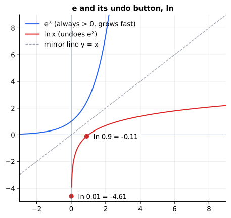
Reading it: the blue curve $e^x$ is always above zero and climbs steeply; every step of 1 to the right multiplies its height by 2.718. The red curve $\ln x$ is the same curve mirrored across the dashed diagonal, because it undoes $e^x$. It only exists for positive inputs, and it dives towards −∞ as its input approaches 0. That dive is the "confidently wrong" penalty in cross-entropy: $-\ln(0.01) = 4.61$, far more than $-\ln(0.9) = 0.11$.
softmax and argmax
softmax turns a list of scores into shares that are positive and sum to
- It is covered step by step, with its symbols decoded, in
primer.ml.attention:
Level 3: the formula and its symbols
$$ \text{softmax}(z)_i = \frac{e^{z_i}}{\sum_{j} e^{z_j}} $$
With the numbers: softmax(2.0, 1.0, 0.5) = (0.63, 0.23, 0.14).
Level 3: in Python
In Python:
import math
z = [2.0, 1.0, 0.5]
# e^(z_i) for each score
exps = [math.exp(z_i) for z_i in z]
# Σ_j e^(z_j)
total = sum(exps)
# each share of the total
[round(e / total, 2) for e in exps]  # → [0.63, 0.23, 0.14]
# argmax: the position of the largest
max(range(len(z)), key=lambda i: z[i])  # → 0
argmax is simpler: it answers "which position holds the largest value?", not "what is the largest value?". argmax(0.1, 7.0, 3.0) = position 2 (index 1 in Python). "Greedy decoding" in a language model is picking the argmax token every step.
In code: softmax subtracts the largest score before exponentiating, so the exponentials cannot overflow; argmax walks the list and remembers the position of the biggest value.
Mean, variance, standard deviation: the middle and the spread
Everyday picture. Two classes both average 70% on a test. In one, everyone scored 68 to 72; in the other, scores ran from 30 to 100. The mean is the same; the spread is not.
Level 3: the formula and its symbols
$$ \mu = \frac{1}{n}\sum_{i=1}^{n} x_i \qquad \sigma^2 = \frac{1}{n}\sum_{i=1}^{n} (x_i - \mu)^2 \qquad \sigma = \sqrt{\sigma^2} $$
Symbols
| Symbol | Meaning |
|---|---|
| $\mu$ (mu) | the mean: the average |
| $\sigma^2$ (sigma squared) | the variance: the average squared distance from the mean; also written $\operatorname{Var}(x)$ |
| $\sigma$ (sigma) | the standard deviation: the typical distance from the mean, in the data's own units |
| $\frac{1}{n}\sum$ | "add them up and divide by how many": an average |
In words: "the mean is the average; the variance is the average squared distance from the mean; the standard deviation is its square root."
With the numbers: for (2, 4, 4, 4, 5, 5, 7, 9): μ = 40 / 8 = 5; the squared distances are (9, 1, 1, 1, 0, 0, 4, 16), which sum to 32, so σ² = 32 / 8 = 4 and σ = 2.
Level 3: in Python
In Python:
import math
x = [2, 4, 4, 4, 5, 5, 7, 9]
n = len(x)
# μ = (1/n) Σ x_i
mu = sum(x) / n
mu  # → 5.0
# the squared distances from μ
[(x_i - mu) ** 2 for x_i in x]  # → [9.0, 1.0, 1.0, 1.0, 0.0, 0.0, 4.0, 16.0]
# σ² = their average
variance = sum((x_i - mu) ** 2 for x_i in x) / n
# σ is its square root
variance, math.sqrt(variance)  # → (4.0, 2.0)
Spread matters constantly in neural networks. If numbers flowing through a
network spread out layer after layer, training blows up; normalization layers
and careful initialization exist to hold σ near 1 (see primer.ml.deep_nets
and the √d_k in primer.ml.attention).
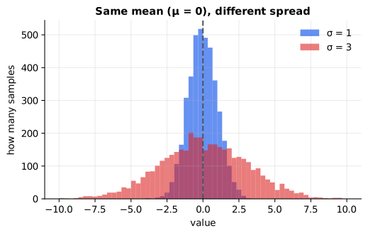
Reading it: both histograms are centred on the same mean (the dashed line), but the blue one is tall and narrow (σ = 1) while the red one is low and wide (σ = 3). The standard deviation is roughly how far from the dashed line a typical sample lands. About two thirds of samples fall within one σ of the mean.
In code: mean, variance and std are the three formulas above, each a short loop built on summation.
Derivatives and gradients: which way is downhill?
Everyday picture. You're on a hillside in thick fog and want to reach the valley. You can't see it, but you can feel the slope under your feet. Take a small step in the steepest downhill direction, feel again, and repeat. That is how every neural network is trained (gradient descent).
The derivative of a function at a point is its slope there: how much the output changes per tiny nudge of the input.
Level 3: the formula and its symbols
$$ f'(x) = \frac{df}{dx} \approx \frac{f(x + h) - f(x - h)}{2h} $$
Symbols
| Symbol | Meaning |
|---|---|
| $f(x)$ | a function: put $x$ in, get a number out |
| $f'(x)$ or $\frac{df}{dx}$ | the derivative: the slope of $f$ at $x$ ("dee f dee x") |
| $h$ | a tiny nudge, like 0.00001 |
| $\approx$ | "approximately equal": exact as $h$ shrinks to 0 |
In words: "nudge the input a hair up and a hair down, and see how much the output changes per unit of nudge."
With the numbers: for $f(x) = x^2$ at $x = 3$: (3.00001² − 2.99999²) / 0.00002 = 6. The slope of $x^2$ at 3 is 6 (the rule is $2x$).
Level 3: in Python
In Python:
def f(x):
    return x ** 2
h = 0.00001
# rise over run across a tiny step
round((f(3 + h) - f(3 - h)) / (2 * h), 6)  # → 6.0
With many inputs, nudge each one separately. The slope in each direction is a partial derivative, written $\frac{\partial f}{\partial x_i}$ (the curly ∂ just means "only this input moves, the others stay fixed"). Collect them into a vector and you have the gradient, written $\nabla f$ ("nabla f" or "grad f"). It points in the steepest uphill direction, so training steps the opposite way:
Level 3: the formula and its symbols
$$ \theta_{\text{new}} = \theta - \eta \, \nabla L(\theta) $$
Symbols
| Symbol | Meaning |
|---|---|
| $\theta$ (theta) | all the model's adjustable numbers (its parameters or weights) |
| $L(\theta)$ | the loss: one number measuring how wrong the model is |
| $\nabla L(\theta)$ | the gradient of the loss: for each weight, how much the loss rises if that weight is nudged up |
| $\eta$ (eta) | the learning rate: how big a step to take, e.g. 0.001 |
In words: "move every weight a small step in the direction that lowers the loss the fastest."
With the numbers: for the bowl $L = x^2 + y^2$ at (1, 2), the gradient is (2, 4), pointing uphill away from the bottom at (0, 0). With η = 0.1, the step goes to (1 − 0.2, 2 − 0.4) = (0.8, 1.6), closer to the bottom.
Level 3: in Python
In Python:
# (x, y)
theta = [1.0, 2.0]
# ∇L for L = x² + y²: each slope is 2 times the value
gradient = [2 * theta[0], 2 * theta[1]]
gradient  # → [2.0, 4.0]
eta = 0.1
# θ_new = θ − η ∇L
[t - eta * g for t, g in zip(theta, gradient)]  # → [0.8, 1.6]
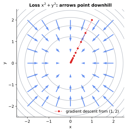
Reading it: the rings are contour lines, as on a hiking map: every point on a ring has the same loss, and the bottom of the bowl is the centre. The arrows show the negative gradient at several spots. They always cross the rings at right angles, pointing straight downhill, and they are longer where the slope is steeper. The dotted path is gradient descent from (1, 2): big steps on the steep outer slope, shrinking steps as the ground flattens near the bottom.
The chain rule says how slopes combine when functions are chained: if
$y = f(g(x))$, then $\frac{dy}{dx} = f'(g(x)) \cdot g'(x)$. Multiply the
slopes along the chain. Backpropagation is the chain rule applied
backwards through every layer of a network, reusing work as it goes (see
primer.ml.neural_net).
In code: derivative measures a slope by nudging the input a hair up and a hair down; gradient does that for each input in turn and collects the slopes into one list.
Probability notation
| You see | Say | Meaning |
|---|---|---|
| $P(A)$ or $p(A)$ | "probability of A" | a number from 0 (never) to 1 (certain) |
| $P(A \mid B)$ | "probability of A given B" | the chance of A once you know B happened |
$P(w_t \mid w_{| "probability of word t given the words before it" |
what a language model computes, one word at a time |
|
| $\mathbb{E}[x]$ | "expected value of x" | the average you'd get over many tries |
| $x \sim \mathcal{N}(0, 1)$ | "x is drawn from a normal distribution with mean 0 and variance 1" | rng.standard_normal() |
Big-O: how cost grows
$O(n^2)$, "order n squared", describes how cost grows as the input
grows, ignoring constant factors. If $n$ doubles, an $O(n)$ cost doubles and
an $O(n^2)$ cost quadruples. Attention is $O(n^2)$ in sequence length, which
is why long context is expensive (primer.ml.attention).
Greek letters you'll meet
| Letter | Name | Usually means |
|---|---|---|
| α | alpha | a mixing weight, or a learning rate |
| β | beta | momentum coefficients in optimizers (β₁, β₂); a strength knob in DPO |
| γ, β | gamma, beta | the learned scale and shift in normalization layers |
| δ | delta | a small change, or an error signal in backprop |
| ε | epsilon | a tiny number added to avoid dividing by zero |
| η | eta | the learning rate |
| θ | theta | all the model's parameters |
| λ | lambda | the strength of a penalty (weight decay) |
| μ | mu | a mean |
| σ | sigma | a standard deviation, or the sigmoid function $\sigma(x) = 1/(1+e^{-x})$ |
| τ | tau | a temperature (sharpness of softmax) |
| ∇ | nabla | the gradient |
| ∂ | "partial" | a partial derivative |
In 20 seconds
- Σ is a loop that adds; Π is a loop that multiplies.
- A dot product multiplies matching entries and adds them up; it measures how much two vectors agree.
- A matrix multiply is a grid of dot products, and it is most of the work a neural network does.
- log undoes e, and it turns products into sums, which is why models work with log-probabilities.
- The gradient points uphill; training steps the other way.
Self-test questions
Read $\sum_{i=1}^{3} i^2$ aloud and evaluate it. "The sum, for i from 1 to 3, of i squared": 1 + 4 + 9 = 14.
What is (2, −1, 3) · (1, 4, 0), and what does its sign tell you? 2 − 4 + 0 = −2. It's negative, so the vectors point somewhat apart.
A is 4 × 3 and B is 3 × 5. What shape is AB? What about BA? AB is 4 × 5. BA is not defined: B's 5 columns don't match A's 4 rows.
Why do language models add log-probabilities instead of multiplying probabilities? A product of thousands of numbers below 1 underflows to 0 in floating point. log(a·b) = log a + log b, so the product becomes a sum of moderate negative numbers.
What does ∇L tell you, and which way does training move? For every weight, how fast the loss rises as that weight increases. Training moves each weight the opposite way, scaled by the learning rate η.
Further reading
- 3Blue1Brown, Essence of Linear Algebra (vectors, matrices, dot products, visually): https://www.3blue1brown.com/topics/linear-algebra
- 3Blue1Brown, Essence of Calculus (derivatives and the chain rule): https://www.3blue1brown.com/topics/calculus
- Khan Academy, Linear algebra: https://www.khanacademy.org/math/linear-algebra
- Deisenroth, Faisal and Ong, Mathematics for Machine Learning (free book): https://mml-book.github.io/
- NumPy, absolute basics for beginners: https://numpy.org/doc/stable/user/absolute_beginners.html
1r""" 2# Math notation, from zero 3 4Run: `python -m primer.notation` 5 6This lesson builds on nothing: it is where the primer's symbols come from. 7 8## Level 1: The practitioner's guide 9 10**In one sentence.** The notation of AI is shorthand for short loops (Σ 11adds a list up, Π multiplies it, a dot product multiplies matching entries 12and adds, ∇ lists the slopes), and the same few dozen symbols fill the 13equations of every paper, the tables of every model card and the parameter 14lists of every API. 15 16**When you need it.** You need it the moment a decision hinges on something 17written in symbols: a model card that says "70B parameters, 4k context, 2.0T 18tokens" (Llama 2's Table 1), an API reference with `temperature`, `top_p` 19and `max_tokens`, a training library's `betas=(0.9, 0.999)`, or a paper 20whose whole claim is one equation. You don't need to derive anything; you 21need to read. The tell: you skip the equation, read the sentence after it, 22and the sentence says "see Equation 1". You don't need this lesson to use a 23chat product, and you don't need proofs, derivations or the appendix of any 24paper to use its result. One number from this lesson shows what reading 25buys: ten agent steps that each succeed 95% of the time all succeed with 26probability 0.95¹⁰ ≈ 0.60 (the demo's first table). Anyone who can read Π 27sees why long chains of steps fail before building one. 28 29**Your options.** Five ways to handle a formula when you meet one, from the 30cheapest to the most certain: 31 32| Option | What it does | What it guarantees | What it costs | Where it lives | 33|---|---|---|---|---| 34| Read the prose, skip the formula | Trusts the author's sentence about what the equation says | Nothing; the prose usually points back at the equation for the part that matters | Free | Your reading | 35| Decode the symbols | Looks each letter up (Σ, η, θ, ‖x‖, ∂) and reads the whole line aloud as a sentence | You know what is added, multiplied or divided, and over what | Minutes, with a symbols table or the Greek-letter table in Level 2 | Your reading | 36| Check the shapes | Follows the sizes through the line: a 4 × 3 matrix times a 3 × 5 matrix is 4 × 5, n tokens by d dimensions stays n by d | Catches most misreadings, because a formula whose shapes don't line up cannot run | One line of arithmetic per formula | The paper's margin, or the shape comments in code | 37| Evaluate it on three numbers | Puts a tiny example through the formula by hand | A number you can compare with the paper's own table | Ten minutes | Paper and pencil | 38| Write it as a loop and run it | Translates Σ into `for`, a dot product into multiply-then-add, and checks the result against NumPy | The definition itself, executable; every function in this lesson is built and tested that way | An hour the first time, minutes after | A notebook | 39 40**How to choose.** Match the effort to what the notation decides. 41 42- A model card or a config file (parameter count, layers, context length): 43 decode the names; no formula is involved. The size words are this lesson's 44 shapes: in Hugging Face's `LlamaConfig`, `hidden_size` 4096 is the vector 45 width d, `num_hidden_layers` 32 is the number of blocks, `vocab_size` 46 32000 is V, and `rms_norm_eps` 1e-6 is the ε that stops a division by 47 zero. 48- An API parameter (`temperature`, `top_p`, `top_k`, `max_tokens`): read 49 the one formula behind it once (softmax, with the scores divided by the 50 temperature; `primer.ml.big_picture` walks it), then follow the vendor's 51 advice. Claude's Messages API documents temperature from 0.0 to 1.0, 52 default 1.0, closer to 0.0 for analytical and multiple-choice work and 53 closer to 1.0 for creative work. 54- A training recipe (η, β₁, β₂, ε, λ, warmup steps, a clipping norm): 55 decode the Greek and copy the values, because these are settings, not 56 derivations. *Attention Is All You Need* trains with Adam at β₁ = 0.9, 57 β₂ = 0.98, ε = 10⁻⁹ and 4000 warmup steps; Llama 2 with AdamW at β₁ = 0.9, 58 β₂ = 0.95, ε = 10⁻⁵, weight decay 0.1 and gradient clipping 1.0. 59 `primer.ml.optimizers` explains each knob. 60- A paper's central equation (a new loss, a new attention variant): 61 evaluate it on three numbers, and write the loop if you will implement it. 62- What you can safely skip: derivations and convergence proofs 63 (appendices), and the notation of the theory (expectations 𝔼, distributions 64 𝒩) until you reproduce a result. What you cannot skip: shapes, Σ, softmax, 65 log, ∇ and the Greek letters that name hyperparameters. 66- Whatever you pick, read every formula aloud as a sentence before deciding 67 it is beyond you. Every formula in this primer has a symbols table and an 68 "In words" line for exactly that. 69 70**What it costs.** Learning the vocabulary costs an afternoon: the whole of 71this lesson is a couple of dozen symbols, and `python -m primer.notation` 72runs every one of them in under a second. Misreading costs more. A 73log-probability is a natural logarithm, so an API that reports a token's 74logprob as −4.61 is saying 1%, and −0.11 is saying 90% (the lesson's *e* and 75log section); read it as base 10 and every confidence you compute is wrong. 76Attention's cost is O(n²) in sequence length (Table 1 of the transformer 77paper gives O(n²·d) per layer), so doubling the context quadruples that part 78of the work, which is the arithmetic behind long-context pricing. And the 79scaling laws are written in this notation: Kaplan et al. (2020) found that 80loss falls as a power law in model size, dataset size and compute, and 81Hoffmann et al. (2022, Chinchilla) that for every doubling of model size the 82training tokens should double too, which is how a 70-billion-parameter model 83came to beat a 280-billion one. A reader who cannot follow N, D and a power 84law cannot check a vendor's claim about either. 85 86**What breaks.** 87 88- **Counting from 1 or from 0.** Mathematics writes $x_1$ for the first 89 entry; Python writes `x[0]`. A position formula copied from a paper into 90 code is off by one until you check which convention it uses. 91- **log means ln.** In ML papers and API responses, log is the natural 92 logarithm. −ln(0.01) = 4.61 and −ln(0.9) = 0.11; that gap is the 93 "confidently wrong" penalty in every training loss. 94- **One letter, several meanings.** β is the momentum coefficient in Adam 95 (β₁, β₂), the learned shift in a normalization layer and the strength knob 96 in DPO; σ is a standard deviation or the sigmoid. The symbols table wins 97 over memory every time. 98- **Shapes that don't line up.** A is 4 × 3 and B is 3 × 5: AB is 4 × 5 and 99 BA does not exist. When a formula's shapes fail, you have misread a 100 transpose, and the code will fail the same way. 101- **Temperature 0 read as determinism.** argmax picks the largest score, but 102 Claude's API reference says results are not fully deterministic even at 103 temperature 0.0, and the pipeline lesson explains why serving hardware 104 makes that so. 105- **Products of probabilities.** The probability of a sentence is a product 106 of thousands of numbers below 1, which underflows to 0 in floating point. 107 That is why models add log-probabilities instead, and why a "score" in a 108 log is negative. 109 110**In the wild.** The transformer paper's Equation 1, softmax(QKᵀ/√d_k)V, 111packs a matrix multiply, a transpose, a square root and a softmax into one 112line, and its Table 1 is the big-O comparison of layer types. Model cards 113and configs carry the shapes: `LlamaConfig` (hidden_size 4096, 114intermediate_size 11008, 32 layers, 32 heads, vocab 32000, initializer_range 1150.02), Llama 2's Table 1 (7B to 70B parameters, 2.0T tokens, learning rates 1163.0 × 10⁻⁴ and 1.5 × 10⁻⁴), the Llama 3 abstract (a dense transformer with 117405B parameters and a 128K-token context). APIs carry the sampling symbols: 118Claude's Messages API (`temperature`, `max_tokens`, `stop_sequences`; models 119released after Claude Opus 4.6 accept only the default temperature of 1.0 120and no `top_k`), Hugging Face's `GenerationConfig` (`do_sample`, otherwise 121greedy; `temperature` 1.0, `top_k` 50, `top_p` 1.0, `max_new_tokens`, 122`repetition_penalty`). Training libraries carry the Greek: PyTorch's 123`AdamW(lr=0.001, betas=(0.9, 0.999), eps=1e-08, weight_decay=0.01)`, 124Hugging Face's `TrainingArguments` (learning_rate 5e-5, adam_beta1 0.9, 125adam_beta2 0.999, adam_epsilon 1e-8, max_grad_norm 1.0). Every value above 126is quoted from the paper or the reference page named beside it; the papers 127are linked from the lessons that build on them. 128 129**Go deeper.** Level 2 builds each symbol as the loop it stands for: Σ and 130Π, the dot product, ‖x‖, matrix multiply and transpose, *e* and log, 131softmax and argmax, mean and spread, derivatives and the gradient, then 132probability notation, big-O and the Greek alphabet, every one with numbers 133you can check by hand and a figure to read. If you only needed to read a 134model card or an API reference, you are done. 135 136## Level 2: How it works, from scratch 137 138Machine learning papers look impenetrable mostly because of **notation**: 139Greek letters, big sigmas, little superscript Ts. Almost every symbol is 140shorthand for a short loop you could write in a few lines of Python. This 141lesson writes each one out as that loop, so that when a formula appears 142elsewhere in this primer you can read it aloud. 143 144Every function below is deliberately written the slow, obvious way, with 145plain Python loops, so the code *is* the definition. The tests check each one 146against NumPy, which does the same thing fast. 147 148## Lists and tables of numbers: vectors and matrices 149 150**Everyday picture.** A **vector** is a list of numbers, like a shopping 151receipt: (apples 3, bread 1, milk 2). A **matrix** is a table of numbers, like 152a spreadsheet with rows and columns. 153 154**Tiny example.** $x = (3, 1, 2)$ is a vector with 3 entries. Its entries are 155written with a small **subscript**: $x_1 = 3$, $x_2 = 1$, $x_3 = 2$. A matrix 156$A$ with 2 rows and 3 columns has **shape** $2 \times 3$, and $A_{2,3}$ means 157"row 2, column 3". 158 159| You see | Say | Python | 160|---|---|---| 161| $x$ (lowercase, sometimes bold **x**) | "the vector x" | `x = [3, 1, 2]` | 162| $x_i$ | "x sub i": the i-th entry | `x[i - 1]` (maths counts from 1, Python from 0) | 163| $A$ (uppercase) | "the matrix A" | `A = [[1, 2, 3], [4, 5, 6]]` | 164| $A_{ij}$ or $A_{i,j}$ | row i, column j | `A[i - 1][j - 1]` | 165| $\mathbb{R}^d$ | "the set of all lists of d real numbers" | any list of d floats | 166| $x \in \mathbb{R}^{768}$ | "x is a list of 768 numbers" | `len(x) == 768` | 167| $n \times d$ | shape: n rows, d columns | `np.zeros((n, d))` | 168 169In practice, a word's embedding is a vector, a batch of embeddings is a 170matrix (one row per word), and a model's weights are mostly matrices. 171 172## Σ (capital sigma): add them all up 173 174**Everyday picture.** Totting up a receipt. 175 176$$ 177\sum_{i=1}^{n} x_i = x_1 + x_2 + \cdots + x_n 178$$ 179 180**Symbols** 181 182| Symbol | Meaning | 183|---|---| 184| $\sum$ | "sum": add up everything that follows | 185| $i = 1$ (below) | start a counter called $i$ at 1 | 186| $n$ (above) | stop after the counter reaches $n$ | 187| $x_i$ | the thing being added on each step | 188| $\cdots$ | "and so on, following the same pattern" | 189 190**In words:** "for i from 1 to n, add up x sub i." 191 192**With the numbers:** $\sum_{i=1}^{4} i = 1 + 2 + 3 + 4 = 10$. In code, Σ is a 193`for` loop with a running total (`summation` below). 194 195**In Python:** 196 197```python 198x = [1, 2, 3, 4] 199total = 0 200# Σ: visit each x_i, from i = 1 to n ... 201for x_i in x: 202 # ... and add it to a running total 203 total += x_i 204total # → 10 205# Python's built-in sum is the same loop 206sum(x) # → 10 207``` 208 209**Π (capital pi)** is the same idea with multiplication: 210$\prod_{i=1}^{4} i = 1 \times 2 \times 3 \times 4 = 24$. It shows up whenever 211independent chances combine. For example, ten steps that each succeed 95% 212of the time all succeed with probability $\prod 0.95 = 0.95^{10} \approx 0.60$. 213This single fact explains why long chains of AI agent steps fail so often 214(`primer.agents.planning`). 215 216**In Python:** 217 218```python 219x = [1, 2, 3, 4] 220product = 1 221# Π: the same loop, multiplying instead of adding 222for x_i in x: 223 product *= x_i 224product # → 24 225# ten steps that each succeed 95% of the time 226round(0.95 ** 10, 2) # → 0.6 227``` 228 229**In code:** `product` is Π written the same way: a loop with a running product that starts at 1. 230 231## The dot product: how much two lists agree 232 233**Everyday picture.** A recipe needs 2 eggs, 3 cups of flour and 1 cup of 234sugar, and eggs cost \$1, flour \$0.50 and sugar \$2 per unit. The total 235cost is 2·1 + 3·0.5 + 1·2 = \$5.50: multiply matching items, then add. That 236is a dot product. 237 238$$ 239a \cdot b = \sum_{i=1}^{d} a_i \, b_i 240$$ 241 242**Symbols** 243 244| Symbol | Meaning | 245|---|---| 246| $a, b$ | two vectors with the same number of entries, $d$ | 247| $a_i b_i$ | the $i$-th entries multiplied together | 248| $\cdot$ | "dot": the whole multiply-then-add operation | 249 250**In words:** "multiply the lists position by position and add up the 251products." 252 253**With the numbers:** $(1, 2) \cdot (3, 0.5) = 1 \cdot 3 + 2 \cdot 0.5 = 4$. 254 255**In Python:** 256 257```python 258a = [1, 2] 259b = [3, 0.5] 260# Σ over i of a_i times b_i 261sum(a_i * b_i for a_i, b_i in zip(a, b)) # → 4.0 262``` 263 264Geometrically, the dot product is large when two arrows point the same way, 265zero when they are at right angles, and negative when they point apart. 266That is why it is the standard similarity score for attention and for 267embeddings. 268 269```mermaid 270flowchart LR 271 A["a = (1, 2)"] --> M1["1 × 3 = 3"] 272 B["b = (3, 0.5)"] --> M1 273 A --> M2["2 × 0.5 = 1"] 274 B --> M2 275 M1 --> S["3 + 1 = 4"] 276 M2 --> S 277``` 278 279**Reading it:** each pair of matching positions meets in a multiply box, 280first entries with first entries and second with second. Every product then 281flows into one addition. A dot product is always this shape: many 282multiplications feeding one sum, however long the lists get. 283 284**In code:** `dot` pairs up matching entries, multiplies them and adds the products with `summation`, refusing lists of different lengths. 285 286## ‖x‖: the length of a vector 287 288**Everyday picture.** Walk 3 blocks east and 4 blocks north. As the crow 289flies, you are 5 blocks from where you started (Pythagoras). 290 291$$ 292\lVert x \rVert = \sqrt{\sum_{i=1}^{d} x_i^2} = \sqrt{x \cdot x} 293$$ 294 295**Symbols** 296 297| Symbol | Meaning | 298|---|---| 299| $\lVert x \rVert$ | the **norm** (length) of $x$, also written $\lVert x \rVert_2$ | 300| $x_i^2$ | the $i$-th entry squared ($x_i \times x_i$) | 301| $\sqrt{\ }$ | square root | 302 303**In words:** "square every entry, add them up, and take the square root." 304 305**With the numbers:** $\lVert (3, 4) \rVert = \sqrt{9 + 16} = 5$ and 306$\lVert (1, 2, 2) \rVert = \sqrt{1 + 4 + 4} = 3$. 307 308**In Python:** 309 310```python 311import math 312def length(x): 313 # √ of Σ x_i² 314 return math.sqrt(sum(x_i ** 2 for x_i in x)) 315length([3, 4]) # → 5.0 316length([1, 2, 2]) # → 3.0 317``` 318 319Dividing a vector by its length gives a **unit vector** of length 1 that 320points the same way. Embedding systems do this constantly, because then the 321dot product measures only direction (see 322`primer.ml.embeddings.similarity`). 323 324**In code:** `norm` is the square root of a vector's dot product with itself. 325 326## Matrix multiply and transpose 327 328**Transpose**, written $A^\top$ ("A transpose"), flips a table on its 329diagonal so rows become columns: a $2 \times 3$ matrix becomes $3 \times 2$. 330 331**Matrix multiply**, written $AB$ with nothing in between, is a whole grid of 332dot products. The cell in row $i$, column $j$ of the answer is row $i$ of $A$ 333dotted with column $j$ of $B$. 334 335$$ 336(AB)_{ij} = \sum_{k=1}^{m} A_{ik} \, B_{kj} 337$$ 338 339**Symbols** 340 341| Symbol | Meaning | 342|---|---| 343| $A$ | an $n \times m$ matrix | 344| $B$ | an $m \times p$ matrix; its row count must equal $A$'s column count, $m$ | 345| $(AB)_{ij}$ | the answer's cell at row $i$, column $j$; the answer is $n \times p$ | 346| $k$ | the counter that walks along row $i$ of $A$ and down column $j$ of $B$ together | 347 348**In words:** "to fill cell (i, j), walk across row i of A and down column j 349of B at the same pace, multiplying and adding." 350 351**With the numbers:** 352$\begin{pmatrix}1&2\\3&4\end{pmatrix}\begin{pmatrix}5&6\\7&8\end{pmatrix} 353= \begin{pmatrix}1\cdot5+2\cdot7 & 1\cdot6+2\cdot8\\ 3\cdot5+4\cdot7 & 3\cdot6+4\cdot8\end{pmatrix} 354= \begin{pmatrix}19&22\\43&50\end{pmatrix}$. 355 356**In Python:** 357 358```python 359A = [[1, 2], [3, 4]] 360B = [[5, 6], [7, 8]] 361# A has m columns, B has m rows: they must match 362m = len(B) 363# (AB)_ij = Σ_k A_ik B_kj 364AB = [[sum(A[i][k] * B[k][j] for k in range(m)) 365 for j in range(len(B[0]))] 366 for i in range(len(A))] 367AB # → [[19, 22], [43, 50]] 368# the transpose: rows become columns 369[list(column) for column in zip(*A)] # → [[1, 3], [2, 4]] 370``` 371 372```mermaid 373flowchart LR 374 R["row 1 of A<br/>(1, 2)"] --> D["dot product<br/>1·5 + 2·7 = 19"] 375 C["column 1 of B<br/>(5, 7)"] --> D 376 D --> O["answer, row 1, column 1 = 19"] 377``` 378 379**Reading it:** a matrix multiply is nothing but this box, repeated for every 380(row, column) pair. The shape rule falls out: the row of A and the column of 381B must be the same length, or there is nothing to pair up. Almost all the 382computation in a neural network is this one operation, which is why GPUs, 383built to do thousands of multiply-adds at once, are the hardware of AI. 384 385**In code:** `transpose` turns columns into rows; `matmul` transposes B once, then fills each cell with one `dot` of a row of A and a column of B. 386 387## e and log: growth, and its undo button 388 389**Everyday picture.** Money in an account that compounds continuously at 390100% a year grows by a factor of **e ≈ 2.718** in one year. $e^x$ is that 391growth run for $x$ years. The **natural logarithm** $\ln y$ (often just 392$\log y$ in ML papers) answers the reverse question: how many years of that 393growth turn 1 into $y$? 394 395| You see | Say | Example | 396|---|---|---| 397| $e^x$ or $\exp(x)$ | "e to the x" | $e^0 = 1$, $e^1 = 2.718$, $e^2 = 7.39$, $e^{-1} = 0.37$ | 398| $\ln y$ or $\log y$ | "log of y" | $\ln 7.39 = 2$, $\ln 1 = 0$, $\ln 0.01 = -4.61$ | 399 400Two facts carry most of machine learning: 401 4021. $e^x$ is **always positive** and **grows fast**, which is why softmax 403 uses it. 4042. $\log(a \times b) = \log a + \log b$. Logs turn multiplying into adding. 405 The probability of a whole sentence is a product of thousands of small 406 numbers, which would underflow to 0 on a computer. Its log is a sum of 407 manageable negative numbers. This is why models work with 408 "log-probabilities", and why the standard training loss is 409 $-\log p$ (see `primer.ml.losses`). 410 411 412 413**Reading it:** the blue curve $e^x$ is always above zero and climbs steeply; 414every step of 1 to the right multiplies its height by 2.718. The red curve 415$\ln x$ is the same curve mirrored across the dashed diagonal, because it 416undoes $e^x$. It only exists for positive inputs, and it dives towards −∞ as 417its input approaches 0. That dive is the "confidently wrong" penalty in 418cross-entropy: $-\ln(0.01) = 4.61$, far more than $-\ln(0.9) = 0.11$. 419 420## softmax and argmax 421 422**softmax** turns a list of scores into shares that are positive and sum to 4231. It is covered step by step, with its symbols decoded, in 424`primer.ml.attention`: 425 426$$ 427\text{softmax}(z)_i = \frac{e^{z_i}}{\sum_{j} e^{z_j}} 428$$ 429 430**With the numbers:** softmax(2.0, 1.0, 0.5) = (0.63, 0.23, 0.14). 431 432**In Python:** 433 434```python 435import math 436z = [2.0, 1.0, 0.5] 437# e^(z_i) for each score 438exps = [math.exp(z_i) for z_i in z] 439# Σ_j e^(z_j) 440total = sum(exps) 441# each share of the total 442[round(e / total, 2) for e in exps] # → [0.63, 0.23, 0.14] 443# argmax: the position of the largest 444max(range(len(z)), key=lambda i: z[i]) # → 0 445``` 446 447**argmax** is simpler: it answers "*which position* holds the largest 448value?", not "what is the largest value?". argmax(0.1, 7.0, 3.0) = position 4492 (index 1 in Python). "Greedy decoding" in a language model is picking the 450argmax token every step. 451 452**In code:** `softmax` subtracts the largest score before exponentiating, so the exponentials cannot overflow; `argmax` walks the list and remembers the position of the biggest value. 453 454## Mean, variance, standard deviation: the middle and the spread 455 456**Everyday picture.** Two classes both average 70% on a test. In one, 457everyone scored 68 to 72; in the other, scores ran from 30 to 100. The 458**mean** is the same; the **spread** is not. 459 460$$ 461\mu = \frac{1}{n}\sum_{i=1}^{n} x_i 462\qquad 463\sigma^2 = \frac{1}{n}\sum_{i=1}^{n} (x_i - \mu)^2 464\qquad 465\sigma = \sqrt{\sigma^2} 466$$ 467 468**Symbols** 469 470| Symbol | Meaning | 471|---|---| 472| $\mu$ (mu) | the **mean**: the average | 473| $\sigma^2$ (sigma squared) | the **variance**: the average squared distance from the mean; also written $\operatorname{Var}(x)$ | 474| $\sigma$ (sigma) | the **standard deviation**: the typical distance from the mean, in the data's own units | 475| $\frac{1}{n}\sum$ | "add them up and divide by how many": an average | 476 477**In words:** "the mean is the average; the variance is the average squared 478distance from the mean; the standard deviation is its square root." 479 480**With the numbers:** for (2, 4, 4, 4, 5, 5, 7, 9): μ = 40 / 8 = 5; the 481squared distances are (9, 1, 1, 1, 0, 0, 4, 16), which sum to 32, so 482σ² = 32 / 8 = 4 and σ = 2. 483 484**In Python:** 485 486```python 487import math 488x = [2, 4, 4, 4, 5, 5, 7, 9] 489n = len(x) 490# μ = (1/n) Σ x_i 491mu = sum(x) / n 492mu # → 5.0 493# the squared distances from μ 494[(x_i - mu) ** 2 for x_i in x] # → [9.0, 1.0, 1.0, 1.0, 0.0, 0.0, 4.0, 16.0] 495# σ² = their average 496variance = sum((x_i - mu) ** 2 for x_i in x) / n 497# σ is its square root 498variance, math.sqrt(variance) # → (4.0, 2.0) 499``` 500 501Spread matters constantly in neural networks. If numbers flowing through a 502network spread out layer after layer, training blows up; normalization layers 503and careful initialization exist to hold σ near 1 (see `primer.ml.deep_nets` 504and the √d_k in `primer.ml.attention`). 505 506 507 508**Reading it:** both histograms are centred on the same mean (the dashed 509line), but the blue one is tall and narrow (σ = 1) while the red one is low 510and wide (σ = 3). The standard deviation is roughly how far from the dashed 511line a typical sample lands. About two thirds of samples fall within one σ 512of the mean. 513 514**In code:** `mean`, `variance` and `std` are the three formulas above, each a short loop built on `summation`. 515 516## Derivatives and gradients: which way is downhill? 517 518**Everyday picture.** You're on a hillside in thick fog and want to reach 519the valley. You can't see it, but you can feel the slope under your feet. 520Take a small step in the steepest downhill direction, feel again, and 521repeat. That is how every neural network is trained (**gradient descent**). 522 523The **derivative** of a function at a point is its slope there: how much the 524output changes per tiny nudge of the input. 525 526$$ 527f'(x) = \frac{df}{dx} \approx \frac{f(x + h) - f(x - h)}{2h} 528$$ 529 530**Symbols** 531 532| Symbol | Meaning | 533|---|---| 534| $f(x)$ | a function: put $x$ in, get a number out | 535| $f'(x)$ or $\frac{df}{dx}$ | the derivative: the slope of $f$ at $x$ ("dee f dee x") | 536| $h$ | a tiny nudge, like 0.00001 | 537| $\approx$ | "approximately equal": exact as $h$ shrinks to 0 | 538 539**In words:** "nudge the input a hair up and a hair down, and see how much 540the output changes per unit of nudge." 541 542**With the numbers:** for $f(x) = x^2$ at $x = 3$: (3.00001² − 2.99999²) / 5430.00002 = 6. The slope of $x^2$ at 3 is 6 (the rule is $2x$). 544 545**In Python:** 546 547```python 548def f(x): 549 return x ** 2 550h = 0.00001 551# rise over run across a tiny step 552round((f(3 + h) - f(3 - h)) / (2 * h), 6) # → 6.0 553``` 554 555With many inputs, nudge each one separately. The slope in each direction is 556a **partial derivative**, written $\frac{\partial f}{\partial x_i}$ (the curly 557∂ just means "only this input moves, the others stay fixed"). Collect them 558into a vector and you have the **gradient**, written $\nabla f$ ("nabla f" or 559"grad f"). It points in the steepest *uphill* direction, so training steps 560the opposite way: 561 562$$ 563\theta_{\text{new}} = \theta - \eta \, \nabla L(\theta) 564$$ 565 566**Symbols** 567 568| Symbol | Meaning | 569|---|---| 570| $\theta$ (theta) | all the model's adjustable numbers (its **parameters** or **weights**) | 571| $L(\theta)$ | the **loss**: one number measuring how wrong the model is | 572| $\nabla L(\theta)$ | the gradient of the loss: for each weight, how much the loss rises if that weight is nudged up | 573| $\eta$ (eta) | the **learning rate**: how big a step to take, e.g. 0.001 | 574 575**In words:** "move every weight a small step in the direction that lowers 576the loss the fastest." 577 578**With the numbers:** for the bowl $L = x^2 + y^2$ at (1, 2), the gradient is 579(2, 4), pointing uphill away from the bottom at (0, 0). With η = 0.1, the 580step goes to (1 − 0.2, 2 − 0.4) = (0.8, 1.6), closer to the bottom. 581 582**In Python:** 583 584```python 585# (x, y) 586theta = [1.0, 2.0] 587# ∇L for L = x² + y²: each slope is 2 times the value 588gradient = [2 * theta[0], 2 * theta[1]] 589gradient # → [2.0, 4.0] 590eta = 0.1 591# θ_new = θ − η ∇L 592[t - eta * g for t, g in zip(theta, gradient)] # → [0.8, 1.6] 593``` 594 595 596 597**Reading it:** the rings are contour lines, as on a hiking map: every point 598on a ring has the same loss, and the bottom of the bowl is the centre. The 599arrows show the negative gradient at several spots. They always cross the 600rings at right angles, pointing straight downhill, and they are longer where 601the slope is steeper. The dotted path is gradient descent from (1, 2): big 602steps on the steep outer slope, shrinking steps as the ground flattens near 603the bottom. 604 605**The chain rule** says how slopes combine when functions are chained: if 606$y = f(g(x))$, then $\frac{dy}{dx} = f'(g(x)) \cdot g'(x)$. Multiply the 607slopes along the chain. **Backpropagation** is the chain rule applied 608backwards through every layer of a network, reusing work as it goes (see 609`primer.ml.neural_net`). 610 611**In code:** `derivative` measures a slope by nudging the input a hair up and a hair down; `gradient` does that for each input in turn and collects the slopes into one list. 612 613## Probability notation 614 615| You see | Say | Meaning | 616|---|---|---| 617| $P(A)$ or $p(A)$ | "probability of A" | a number from 0 (never) to 1 (certain) | 618| $P(A \mid B)$ | "probability of A given B" | the chance of A once you know B happened | 619| $P(w_t \mid w_{<t})$ | "probability of word t given the words before it" | what a language model computes, one word at a time | 620| $\mathbb{E}[x]$ | "expected value of x" | the average you'd get over many tries | 621| $x \sim \mathcal{N}(0, 1)$ | "x is drawn from a normal distribution with mean 0 and variance 1" | `rng.standard_normal()` | 622 623## Big-O: how cost grows 624 625$O(n^2)$, "order n squared", describes how cost **grows** as the input 626grows, ignoring constant factors. If $n$ doubles, an $O(n)$ cost doubles and 627an $O(n^2)$ cost quadruples. Attention is $O(n^2)$ in sequence length, which 628is why long context is expensive (`primer.ml.attention`). 629 630## Greek letters you'll meet 631 632| Letter | Name | Usually means | 633|---|---|---| 634| α | alpha | a mixing weight, or a learning rate | 635| β | beta | momentum coefficients in optimizers (β₁, β₂); a strength knob in DPO | 636| γ, β | gamma, beta | the learned scale and shift in normalization layers | 637| δ | delta | a small change, or an error signal in backprop | 638| ε | epsilon | a tiny number added to avoid dividing by zero | 639| η | eta | the learning rate | 640| θ | theta | all the model's parameters | 641| λ | lambda | the strength of a penalty (weight decay) | 642| μ | mu | a mean | 643| σ | sigma | a standard deviation, or the sigmoid function $\sigma(x) = 1/(1+e^{-x})$ | 644| τ | tau | a temperature (sharpness of softmax) | 645| ∇ | nabla | the gradient | 646| ∂ | "partial" | a partial derivative | 647 648## In 20 seconds 649 650- Σ is a loop that adds; Π is a loop that multiplies. 651- A dot product multiplies matching entries and adds them up; it measures 652 how much two vectors agree. 653- A matrix multiply is a grid of dot products, and it is most of the work a 654 neural network does. 655- log undoes e, and it turns products into sums, which is why models work 656 with log-probabilities. 657- The gradient points uphill; training steps the other way. 658 659## Self-test questions 660 661**Read $\sum_{i=1}^{3} i^2$ aloud and evaluate it.** 662"The sum, for i from 1 to 3, of i squared": 1 + 4 + 9 = 14. 663 664**What is (2, −1, 3) · (1, 4, 0), and what does its sign tell you?** 6652 − 4 + 0 = −2. It's negative, so the vectors point somewhat apart. 666 667**A is 4 × 3 and B is 3 × 5. What shape is AB? What about BA?** 668AB is 4 × 5. BA is not defined: B's 5 columns don't match A's 4 rows. 669 670**Why do language models add log-probabilities instead of multiplying 671probabilities?** 672A product of thousands of numbers below 1 underflows to 0 in floating point. 673log(a·b) = log a + log b, so the product becomes a sum of moderate 674negative numbers. 675 676**What does ∇L tell you, and which way does training move?** 677For every weight, how fast the loss rises as that weight increases. Training 678moves each weight the opposite way, scaled by the learning rate η. 679 680## Further reading 681 682- 3Blue1Brown, *Essence of Linear Algebra* (vectors, matrices, dot products, visually): https://www.3blue1brown.com/topics/linear-algebra 683- 3Blue1Brown, *Essence of Calculus* (derivatives and the chain rule): https://www.3blue1brown.com/topics/calculus 684- Khan Academy, *Linear algebra*: https://www.khanacademy.org/math/linear-algebra 685- Deisenroth, Faisal and Ong, *Mathematics for Machine Learning* (free book): https://mml-book.github.io/ 686- NumPy, absolute basics for beginners: https://numpy.org/doc/stable/user/absolute_beginners.html 687""" 688 689from __future__ import annotations 690 691import math 692from typing import Callable, Sequence 693 694from primer._show import banner, say, table, takeaway 695 696Vector = Sequence[float] 697Matrix = Sequence[Sequence[float]] 698 699 700# --------------------------------------------------------------------------- 701# Σ and Π 702# --------------------------------------------------------------------------- 703 704 705def summation(xs: Vector) -> float: 706 """Σ xᵢ: a loop with a running total that starts at 0.""" 707 total = 0 708 for x in xs: 709 total += x 710 return total 711 712 713def product(xs: Vector) -> float: 714 """Π xᵢ: a loop with a running product that starts at 1 (multiplying by 1 changes nothing).""" 715 result = 1 716 for x in xs: 717 result *= x 718 return result 719 720 721# --------------------------------------------------------------------------- 722# Vectors 723# --------------------------------------------------------------------------- 724 725 726def dot(a: Vector, b: Vector) -> float: 727 """a · b = Σ aᵢ bᵢ. Lists must be the same length, or there's nothing to pair up.""" 728 if len(a) != len(b): 729 raise ValueError(f"dot product needs equal lengths, got {len(a)} and {len(b)}") 730 return summation([ai * bi for ai, bi in zip(a, b)]) 731 732 733def norm(x: Vector) -> float: 734 """‖x‖ = √(x · x): Pythagoras in any number of dimensions.""" 735 return math.sqrt(dot(x, x)) 736 737 738# --------------------------------------------------------------------------- 739# Matrices 740# --------------------------------------------------------------------------- 741 742 743def transpose(A: Matrix) -> list[list[float]]: 744 """Aᵀ: row i of the answer is column i of A.""" 745 return [[row[j] for row in A] for j in range(len(A[0]))] 746 747 748def matmul(A: Matrix, B: Matrix) -> list[list[float]]: 749 """(AB)ᵢⱼ = row i of A · column j of B. A is n×m, B must be m×p, the answer is n×p.""" 750 if len(A[0]) != len(B): 751 raise ValueError(f"inner sizes differ: A has {len(A[0])} columns, B has {len(B)} rows") 752 columns_of_B = transpose(B) 753 return [[dot(row, col) for col in columns_of_B] for row in A] 754 755 756# --------------------------------------------------------------------------- 757# softmax and argmax 758# --------------------------------------------------------------------------- 759 760 761def softmax(z: Vector) -> list[float]: 762 """e^zᵢ / Σⱼ e^zⱼ. Subtracting max(z) first changes nothing mathematically 763 (it cancels top and bottom) but keeps e^z from overflowing.""" 764 m = max(z) 765 exps = [math.exp(zi - m) for zi in z] 766 total = summation(exps) 767 return [e / total for e in exps] 768 769 770def argmax(xs: Vector) -> int: 771 """The *position* of the largest value (0-based, as Python counts).""" 772 best = 0 773 for i in range(1, len(xs)): 774 if xs[i] > xs[best]: 775 best = i 776 return best 777 778 779# --------------------------------------------------------------------------- 780# Mean and spread 781# --------------------------------------------------------------------------- 782 783 784def mean(xs: Vector) -> float: 785 """μ = (1/n) Σ xᵢ.""" 786 return summation(xs) / len(xs) 787 788 789def variance(xs: Vector) -> float: 790 """σ² = (1/n) Σ (xᵢ − μ)²: the average squared distance from the mean.""" 791 mu = mean(xs) 792 return mean([(x - mu) ** 2 for x in xs]) 793 794 795def std(xs: Vector) -> float: 796 """σ = √σ²: the typical distance from the mean, in the data's own units.""" 797 return math.sqrt(variance(xs)) 798 799 800# --------------------------------------------------------------------------- 801# Derivatives and gradients 802# --------------------------------------------------------------------------- 803 804 805def derivative(f: Callable[[float], float], x: float, h: float = 1e-5) -> float: 806 """f'(x) ≈ (f(x+h) − f(x−h)) / 2h. Nudging both ways (a "central difference") 807 is far more accurate than nudging one way.""" 808 return (f(x + h) - f(x - h)) / (2 * h) 809 810 811def gradient(f: Callable[[list[float]], float], x: Vector, h: float = 1e-5) -> list[float]: 812 """∇f: one partial derivative per input, each found by nudging only that input.""" 813 grads = [] 814 for i in range(len(x)): 815 up, down = list(x), list(x) 816 up[i] += h 817 down[i] -= h 818 grads.append((f(up) - f(down)) / (2 * h)) 819 return grads 820 821 822# --------------------------------------------------------------------------- 823# Figures 824# --------------------------------------------------------------------------- 825 826 827def figures() -> dict: 828 """Plot this lesson's data (matplotlib is imported here only).""" 829 import matplotlib 830 831 matplotlib.use("Agg") 832 import matplotlib.pyplot as plt 833 import numpy as np 834 835 figs = {} 836 837 # e^x and ln x, mirrored across y = x 838 fig, ax = plt.subplots(figsize=(5.5, 5)) 839 xs = np.linspace(-3, np.log(9), 200) # e^x reaches the chart's top, 9, at x = ln 9 840 ax.plot(xs, np.exp(xs), label="$e^x$ (always > 0, grows fast)") 841 pos = np.linspace(0.02, 9, 300) 842 ax.plot(pos, np.log(pos), label=r"$\ln x$ (undoes $e^x$)") 843 ax.plot([-3, 9], [-3, 9], ls="--", color="#9ca3af", lw=1, label="mirror line y = x") 844 for p in (0.9, 0.01): 845 ax.plot(p, np.log(p), "o", color="#dc2626") 846 ax.annotate(f"ln {p} = {np.log(p):.2f}", (p, np.log(p)), xytext=(10, -4), textcoords="offset points", zorder=3, bbox=dict(facecolor="white", edgecolor="none", pad=1)) 847 ax.set_xlim(-3, 9) 848 ax.set_ylim(-5, 9) 849 ax.axhline(0, color="#4b5563", lw=0.8) 850 ax.axvline(0, color="#4b5563", lw=0.8) 851 ax.set_title("e and its undo button, ln") 852 ax.legend(frameon=False, loc="upper left") 853 figs["exp_log"] = fig 854 855 # same mean, different spread 856 rng = np.random.default_rng(0) 857 fig, ax = plt.subplots(figsize=(6, 3.4)) 858 bins = np.linspace(-10, 10, 61) 859 ax.hist(rng.normal(0, 1, 4000), bins=bins, alpha=0.7, label="σ = 1") 860 ax.hist(rng.normal(0, 3, 4000), bins=bins, alpha=0.6, label="σ = 3") 861 ax.axvline(0, ls="--", color="#4b5563") 862 ax.set_xlabel("value") 863 ax.set_ylabel("how many samples") 864 ax.set_title("Same mean (μ = 0), different spread") 865 ax.legend(frameon=False) 866 figs["spread"] = fig 867 868 # gradient descent on a bowl 869 fig, ax = plt.subplots(figsize=(5.5, 5)) 870 g = np.linspace(-2.5, 2.5, 200) 871 X, Y = np.meshgrid(g, g) 872 ax.contour(X, Y, X**2 + Y**2, levels=10, colors="#9ca3af", linewidths=0.8) 873 q = np.linspace(-2, 2, 7) 874 QX, QY = np.meshgrid(q, q) 875 ax.quiver(QX, QY, -2 * QX, -2 * QY, color="#2563eb", alpha=0.7, angles="xy", scale_units="xy", scale=8) 876 path = [np.array([1.0, 2.0])] 877 for _ in range(12): 878 path.append(path[-1] - 0.15 * np.array(gradient(lambda v: v[0] ** 2 + v[1] ** 2, path[-1].tolist()))) 879 path = np.array(path) 880 ax.plot(path[:, 0], path[:, 1], "o:", color="#dc2626", ms=4, label="gradient descent from (1, 2)") 881 ax.set_aspect("equal") 882 ax.set_xlabel("x") 883 ax.set_ylabel("y") 884 ax.set_title("Loss $x^2+y^2$: arrows point downhill") 885 ax.legend(frameon=False, loc="lower right") 886 ax.grid(False) 887 figs["gradient_descent"] = fig 888 889 return figs 890 891 892# --------------------------------------------------------------------------- 893# Walkthrough 894# --------------------------------------------------------------------------- 895 896 897def demo() -> None: 898 banner("1. Σ is a loop that adds, Π is a loop that multiplies") 899 say("Σ over 1..4 and Π over 1..4, then the chance that 10 steps at 95% all succeed:") 900 table(["expression", "value"], [("Σ i, i=1..4", summation([1, 2, 3, 4])), ("Π i, i=1..4", product([1, 2, 3, 4])), ("0.95^10", product([0.95] * 10))], floatfmt=".3f") 901 takeaway("A 95%-reliable step repeated 10 times succeeds only 60% of the time.") 902 903 banner("2. Dot product and length") 904 table( 905 ["expression", "working", "value"], 906 [("(1,2)·(3,0.5)", "1·3 + 2·0.5", dot([1, 2], [3, 0.5])), ("‖(3,4)‖", "√(9+16)", norm([3, 4])), ("‖(1,2,2)‖", "√(1+4+4)", norm([1, 2, 2]))], 907 floatfmt=".1f", 908 ) 909 910 banner("3. Matrix multiply is a grid of dot products") 911 A, B = [[1, 2], [3, 4]], [[5, 6], [7, 8]] 912 say(f"A = {A}, B = {B}. Cell (1,1) = row 1 of A · column 1 of B = 1·5 + 2·7 = 19.") 913 say(f"AB = {matmul(A, B)}. Aᵀ = {transpose(A)}.") 914 915 banner("4. softmax and argmax") 916 s = softmax([2.0, 1.0, 0.5]) 917 say(f"softmax(2.0, 1.0, 0.5) = ({s[0]:.2f}, {s[1]:.2f}, {s[2]:.2f}), which sums to {sum(s):.2f}.") 918 say(f"argmax(0.1, 7.0, 3.0) = {argmax([0.1, 7.0, 3.0])}: the position of the biggest value, not the value.") 919 920 banner("5. Middle and spread") 921 data = [2, 4, 4, 4, 5, 5, 7, 9] 922 table(["data", "mean μ", "variance σ²", "std σ"], [(data, mean(data), variance(data), std(data))], floatfmt=".1f") 923 924 banner("6. Slopes: derivative and gradient") 925 say(f"Slope of x² at x=3: {derivative(lambda x: x * x, 3.0):.4f} (the rule 2x says 6).") 926 gr = gradient(lambda v: v[0] ** 2 + v[1] ** 2, [1.0, 2.0]) 927 say(f"Gradient of x²+y² at (1,2): ({gr[0]:.2f}, {gr[1]:.2f}). It points uphill; training steps the other way.") 928 takeaway("Every symbol in an ML paper is shorthand for a short loop. Read it aloud, then write the loop.") 929 930 931if __name__ == "__main__": 932 demo()
706def summation(xs: Vector) -> float:
707    """Σ xᵢ: a loop with a running total that starts at 0."""
708    total = 0
709    for x in xs:
710        total += x
711    return total
Σ xᵢ: a loop with a running total that starts at 0.
714def product(xs: Vector) -> float:
715    """Π xᵢ: a loop with a running product that starts at 1 (multiplying by 1 changes nothing)."""
716    result = 1
717    for x in xs:
718        result *= x
719    return result
Π xᵢ: a loop with a running product that starts at 1 (multiplying by 1 changes nothing).
727def dot(a: Vector, b: Vector) -> float:
728    """a · b = Σ aᵢ bᵢ. Lists must be the same length, or there's nothing to pair up."""
729    if len(a) != len(b):
730        raise ValueError(f"dot product needs equal lengths, got {len(a)} and {len(b)}")
731    return summation([ai * bi for ai, bi in zip(a, b)])
a · b = Σ aᵢ bᵢ. Lists must be the same length, or there's nothing to pair up.
734def norm(x: Vector) -> float:
735    """‖x‖ = √(x · x): Pythagoras in any number of dimensions."""
736    return math.sqrt(dot(x, x))
‖x‖ = √(x · x): Pythagoras in any number of dimensions.
744def transpose(A: Matrix) -> list[list[float]]:
745    """Aᵀ: row i of the answer is column i of A."""
746    return [[row[j] for row in A] for j in range(len(A[0]))]
Aᵀ: row i of the answer is column i of A.
749def matmul(A: Matrix, B: Matrix) -> list[list[float]]:
750    """(AB)ᵢⱼ = row i of A · column j of B. A is n×m, B must be m×p, the answer is n×p."""
751    if len(A[0]) != len(B):
752        raise ValueError(f"inner sizes differ: A has {len(A[0])} columns, B has {len(B)} rows")
753    columns_of_B = transpose(B)
754    return [[dot(row, col) for col in columns_of_B] for row in A]
(AB)ᵢⱼ = row i of A · column j of B. A is n×m, B must be m×p, the answer is n×p.
762def softmax(z: Vector) -> list[float]:
763    """e^zᵢ / Σⱼ e^zⱼ. Subtracting max(z) first changes nothing mathematically
764    (it cancels top and bottom) but keeps e^z from overflowing."""
765    m = max(z)
766    exps = [math.exp(zi - m) for zi in z]
767    total = summation(exps)
768    return [e / total for e in exps]
e^zᵢ / Σⱼ e^zⱼ. Subtracting max(z) first changes nothing mathematically (it cancels top and bottom) but keeps e^z from overflowing.
771def argmax(xs: Vector) -> int:
772    """The *position* of the largest value (0-based, as Python counts)."""
773    best = 0
774    for i in range(1, len(xs)):
775        if xs[i] > xs[best]:
776            best = i
777    return best
The position of the largest value (0-based, as Python counts).
μ = (1/n) Σ xᵢ.
790def variance(xs: Vector) -> float:
791    """σ² = (1/n) Σ (xᵢ − μ)²: the average squared distance from the mean."""
792    mu = mean(xs)
793    return mean([(x - mu) ** 2 for x in xs])
σ² = (1/n) Σ (xᵢ − μ)²: the average squared distance from the mean.
796def std(xs: Vector) -> float:
797    """σ = √σ²: the typical distance from the mean, in the data's own units."""
798    return math.sqrt(variance(xs))
σ = √σ²: the typical distance from the mean, in the data's own units.
806def derivative(f: Callable[[float], float], x: float, h: float = 1e-5) -> float:
807    """f'(x) ≈ (f(x+h) − f(x−h)) / 2h. Nudging both ways (a "central difference")
808    is far more accurate than nudging one way."""
809    return (f(x + h) - f(x - h)) / (2 * h)
f'(x) ≈ (f(x+h) − f(x−h)) / 2h. Nudging both ways (a "central difference") is far more accurate than nudging one way.
812def gradient(f: Callable[[list[float]], float], x: Vector, h: float = 1e-5) -> list[float]:
813    """∇f: one partial derivative per input, each found by nudging only that input."""
814    grads = []
815    for i in range(len(x)):
816        up, down = list(x), list(x)
817        up[i] += h
818        down[i] -= h
819        grads.append((f(up) - f(down)) / (2 * h))
820    return grads
∇f: one partial derivative per input, each found by nudging only that input.
828def figures() -> dict:
829    """Plot this lesson's data (matplotlib is imported here only)."""
830    import matplotlib
831
832    matplotlib.use("Agg")
833    import matplotlib.pyplot as plt
834    import numpy as np
835
836    figs = {}
837
838    # e^x and ln x, mirrored across y = x
839    fig, ax = plt.subplots(figsize=(5.5, 5))
840    xs = np.linspace(-3, np.log(9), 200)  # e^x reaches the chart's top, 9, at x = ln 9
841    ax.plot(xs, np.exp(xs), label="$e^x$ (always > 0, grows fast)")
842    pos = np.linspace(0.02, 9, 300)
843    ax.plot(pos, np.log(pos), label=r"$\ln x$ (undoes $e^x$)")
844    ax.plot([-3, 9], [-3, 9], ls="--", color="#9ca3af", lw=1, label="mirror line y = x")
845    for p in (0.9, 0.01):
846        ax.plot(p, np.log(p), "o", color="#dc2626")
847        ax.annotate(f"ln {p} = {np.log(p):.2f}", (p, np.log(p)), xytext=(10, -4), textcoords="offset points", zorder=3, bbox=dict(facecolor="white", edgecolor="none", pad=1))
848    ax.set_xlim(-3, 9)
849    ax.set_ylim(-5, 9)
850    ax.axhline(0, color="#4b5563", lw=0.8)
851    ax.axvline(0, color="#4b5563", lw=0.8)
852    ax.set_title("e and its undo button, ln")
853    ax.legend(frameon=False, loc="upper left")
854    figs["exp_log"] = fig
855
856    # same mean, different spread
857    rng = np.random.default_rng(0)
858    fig, ax = plt.subplots(figsize=(6, 3.4))
859    bins = np.linspace(-10, 10, 61)
860    ax.hist(rng.normal(0, 1, 4000), bins=bins, alpha=0.7, label="σ = 1")
861    ax.hist(rng.normal(0, 3, 4000), bins=bins, alpha=0.6, label="σ = 3")
862    ax.axvline(0, ls="--", color="#4b5563")
863    ax.set_xlabel("value")
864    ax.set_ylabel("how many samples")
865    ax.set_title("Same mean (μ = 0), different spread")
866    ax.legend(frameon=False)
867    figs["spread"] = fig
868
869    # gradient descent on a bowl
870    fig, ax = plt.subplots(figsize=(5.5, 5))
871    g = np.linspace(-2.5, 2.5, 200)
872    X, Y = np.meshgrid(g, g)
873    ax.contour(X, Y, X**2 + Y**2, levels=10, colors="#9ca3af", linewidths=0.8)
874    q = np.linspace(-2, 2, 7)
875    QX, QY = np.meshgrid(q, q)
876    ax.quiver(QX, QY, -2 * QX, -2 * QY, color="#2563eb", alpha=0.7, angles="xy", scale_units="xy", scale=8)
877    path = [np.array([1.0, 2.0])]
878    for _ in range(12):
879        path.append(path[-1] - 0.15 * np.array(gradient(lambda v: v[0] ** 2 + v[1] ** 2, path[-1].tolist())))
880    path = np.array(path)
881    ax.plot(path[:, 0], path[:, 1], "o:", color="#dc2626", ms=4, label="gradient descent from (1, 2)")
882    ax.set_aspect("equal")
883    ax.set_xlabel("x")
884    ax.set_ylabel("y")
885    ax.set_title("Loss $x^2+y^2$: arrows point downhill")
886    ax.legend(frameon=False, loc="lower right")
887    ax.grid(False)
888    figs["gradient_descent"] = fig
889
890    return figs
Plot this lesson's data (matplotlib is imported here only).
898def demo() -> None:
899    banner("1. Σ is a loop that adds, Π is a loop that multiplies")
900    say("Σ over 1..4 and Π over 1..4, then the chance that 10 steps at 95% all succeed:")
901    table(["expression", "value"], [("Σ i, i=1..4", summation([1, 2, 3, 4])), ("Π i, i=1..4", product([1, 2, 3, 4])), ("0.95^10", product([0.95] * 10))], floatfmt=".3f")
902    takeaway("A 95%-reliable step repeated 10 times succeeds only 60% of the time.")
903
904    banner("2. Dot product and length")
905    table(
906        ["expression", "working", "value"],
907        [("(1,2)·(3,0.5)", "1·3 + 2·0.5", dot([1, 2], [3, 0.5])), ("‖(3,4)‖", "√(9+16)", norm([3, 4])), ("‖(1,2,2)‖", "√(1+4+4)", norm([1, 2, 2]))],
908        floatfmt=".1f",
909    )
910
911    banner("3. Matrix multiply is a grid of dot products")
912    A, B = [[1, 2], [3, 4]], [[5, 6], [7, 8]]
913    say(f"A = {A}, B = {B}. Cell (1,1) = row 1 of A · column 1 of B = 1·5 + 2·7 = 19.")
914    say(f"AB = {matmul(A, B)}.  Aᵀ = {transpose(A)}.")
915
916    banner("4. softmax and argmax")
917    s = softmax([2.0, 1.0, 0.5])
918    say(f"softmax(2.0, 1.0, 0.5) = ({s[0]:.2f}, {s[1]:.2f}, {s[2]:.2f}), which sums to {sum(s):.2f}.")
919    say(f"argmax(0.1, 7.0, 3.0) = {argmax([0.1, 7.0, 3.0])}: the position of the biggest value, not the value.")
920
921    banner("5. Middle and spread")
922    data = [2, 4, 4, 4, 5, 5, 7, 9]
923    table(["data", "mean μ", "variance σ²", "std σ"], [(data, mean(data), variance(data), std(data))], floatfmt=".1f")
924
925    banner("6. Slopes: derivative and gradient")
926    say(f"Slope of x² at x=3: {derivative(lambda x: x * x, 3.0):.4f} (the rule 2x says 6).")
927    gr = gradient(lambda v: v[0] ** 2 + v[1] ** 2, [1.0, 2.0])
928    say(f"Gradient of x²+y² at (1,2): ({gr[0]:.2f}, {gr[1]:.2f}). It points uphill; training steps the other way.")
929    takeaway("Every symbol in an ML paper is shorthand for a short loop. Read it aloud, then write the loop.")