primer.ml.regularization
Regularization: learning the pattern instead of memorising the examples
Run: python -m primer.ml.regularization
New to the notation? primer.notation explains every symbol used here from
zero. This lesson builds on the losses in primer.ml.losses and the
training loop in primer.ml.neural_net.
Level 1: The practitioner's guide
In one sentence. Regularization is everything you do to make a model learn the pattern in its training data rather than memorise the examples, and the way you know it is working is the gap between the error on data the model trained on and the error on data it has never seen.
When you need it. Whenever you train or fine-tune anything on less data than the model could memorise, which in practice is always: a fine-tune on a few thousand examples, a classifier on a table of ten thousand rows, a forecasting model on a year of history. The tell is a training error that keeps falling while the validation error turns and climbs. This lesson's polynomial sweep shows the whole story in one table: at degree 5 the training error is 0.013 and the validation error 0.057; at degree 9 the training error has dropped to 0.004 and the validation error has risen twelve-fold to 0.71; at degree 11 the training error is zero and the validation error is 7,631. Its over-sized network bottoms out on validation near epoch 300 and gets steadily worse for the next 1,700 epochs while its training loss keeps improving. The other tell is the opposite one, and it hides in a good offline score: a model that looked superb in evaluation and collapsed in production has usually seen the answers, and that is leakage, which the same lesson covers. You do not need more regularization when both errors are high; that is underfitting, and it wants more capacity, more features or more training, the opposite fix.
Your options. From the cheapest to the most involved:
| Option | What it does | What it guarantees | What it costs | Where it lives |
|---|---|---|---|---|
| A held-out validation set (and a test set touched once) | Measures the gap that every other option is judged by | An honest estimate, as long as the test set is not used to choose | 15% to 30% of your data, and discipline | Your data pipeline |
| Early stopping | Watches validation loss, stops after patience bad checks, restores the best weights |
You ship the best model seen, not the last | A validation pass per epoch; nothing in the model | The training loop: a callback in every framework |
| More data, or augmented data | Averages the noise away | Tames variance in flexible models; does nothing for a model too simple to fit the pattern | Collection or labelling time | Your data |
| L2 penalty (weight decay) | Taxes the square of every weight, so all of them shrink a little | Smaller, smoother weights; nothing is eliminated | One hyperparameter, λ | The optimiser: on by default in AdamW |
| Dropout | Zeroes each activation with probability p on every training step, scaled so evaluation is a plain pass-through | No neuron becomes indispensable | Slower convergence; a bug if left on at evaluation | The model, between layers |
| L1 penalty (lasso) | Charges a flat fee per unit of weight, so small weights go to exactly zero | A sparse model that names its features | Harder optimisation; one hyperparameter | Linear and tabular models, feature selection |
| Less capacity | A smaller model, a lower polynomial degree, fewer features | Less to memorise with | Possibly too little to learn the pattern | The architecture |
| Cross-validation | Trains k models, each with one fold held out, and averages their scores | A steadier estimate than one split when data is small | k training runs | Small tabular problems; scikit-learn's cross-validation guide |
| Leak-proof splitting | Deduplicates before splitting, splits by time or by user, drops features unknown at prediction time | An offline score that survives production | Thinking about the timeline of every feature | Your data pipeline, before any training |
How to choose. Diagnose first, because the two failures want opposite cures.
- Both errors high: underfitting. Add capacity, features or training time. Regularizing further makes it worse.
- Training low, validation high: overfitting. Early stopping first, because it costs nothing; then weight decay (which you probably already have) and dropout; then more data if you can get it.
- A tabular model you must explain, or hundreds of features of which a few matter: L1, which in this lesson zeroes 5 of 7 useless weights while L2 zeroes none.
- Fewer than a few thousand examples: cross-validate rather than trust one split.
- A model that was wonderful offline: before celebrating, check for twins across the split and for columns filled in after the outcome.
- Whatever you pick, the test set is touched once, at the end. Every
decision made by looking at it turns it into a second validation set, and
the benchmark version of this failure is Goodhart's law in
primer.ml.benchmarks.
What it costs. Early stopping costs one validation pass per epoch and stops training sooner, so it usually saves compute. Weight decay and L1 cost nothing at inference and one hyperparameter each; PyTorch's AdamW defaults weight decay to 0.01. Dropout slows training, because each step trains a thinned network, and the original transformer used p = 0.1 rather than anything heavier. Cross-validation multiplies training cost by the number of folds. The dear cost is data: the validation and test sets are examples you cannot train on, and with 100 examples a 70 / 15 / 15 split leaves 15 for each. Leakage costs the most of all, late: this lesson's fraud model with a future feature scores 98% offline and 49% in production, worse than the honest model's 61%.
What breaks.
- Dropout left on at evaluation. Predictions become noisy and change
from call to call. Switch the model to evaluation mode; the lesson's
dropoutpasses activations through unchanged there. - Early stopping with no restore. Stopping is half the job; the weights at the stop are the ones that just failed twice. Keep the snapshot from the best check.
- Patience too short. A noisy validation curve stops training on a blip. Smooth it, or raise the patience.
- Tuning against the test set. Each look fits the model to it a little. Choose with validation, report with test.
- Duplicates across the split. A nearest-neighbour memoriser scores 87% on data whose labels are 30% noise, when no honest model can beat about 70%; deduplicated, it scores 50%. Deduplicate before splitting.
- A feature from the future.
chargeback_filedis recorded after the outcome. Ask of every column: would I know this at prediction time? - A random split on time-ordered data. Predicting next month from a shuffle of all months is a leak. Split by time when the task is the future, by user when the task is new users.
- Regularizing an underfit model. It cannot get better by learning less. Look at both curves before reaching for the penalty.
In the wild. Weight decay is on by default in the optimisers that train
transformers: torch.optim.AdamW takes weight_decay with a default of
0.01, and primer.ml.optimizers shows why decoupling it from the gradient
step mattered. Early stopping is a callback everywhere it is offered;
Keras's EarlyStopping has patience and restore_best_weights, which
default to 0 and False, so a naive call gets neither. Dropout (Srivastava
et al., 2014) trains at p = 0.1 in the original transformer and is switched
off by model.eval() in PyTorch. The lasso is Tibshirani (1996), and
scikit-learn's cross-validation guide is the standard reference for folds
that respect groups and time. Kapoor and Narayanan (2022) catalogued the
kinds of leakage and how widely they inflate published results, and Belkin
et al. (2018) documented double descent, where very over-parameterised
models generalise well again, which is why the modern recipe is a large
model plus regularization rather than a small model.
Go deeper. Level 2 fits the memorising cubic by hand, sweeps polynomial degree to draw the valley in validation error, replays early stopping on a list of losses, splits error into bias and variance over 300 training sets, builds dropout and the two penalties in a few lines each, cuts data into folds, and reproduces both leaks with a nearest-neighbour memoriser. If you only needed to diagnose a curve and pick a fix, you are done.
Level 2: How it works, from scratch
Two students prepare for an exam. One learns the ideas. The other memorises last year's paper, answer by answer, and scores 100% on it in practice. On the real exam, with new questions, the first student does fine and the second falls apart. A model that memorises its training examples, noise and all, instead of learning the pattern behind them is overfitting. It looks brilliant on the data it has seen and fails on data it hasn't. Regularization is everything we do to push a model toward the first student.
Worked example: four training points (0, 0), (1, 1), (2, 0), (3, 1), a zig-zag that is really "about 0.5, plus noise".
| model | error on the 4 training points | prediction at x = 4 |
|---|---|---|
| flat line at 0.5 (the pattern) | 0.25 | 0.5 |
| cubic through all four points (memorised) | 0 | 8 |
The cubic is perfect on the training data and absurd one step beyond it. You can check the 8 by hand with a difference table: the values 0, 1, 0, 1 have differences 1, −1, 1, then −2, 2, then 4; a cubic keeps that last difference constant, so extending the table gives 6, then 7, then 8.
flowchart LR
  D["Training data =<br/>pattern + noise"] --> M{Model capacity}
  M -->|too little| U["Underfits:<br/>misses the pattern"]
  M -->|about right| G["Generalizes:<br/>learns the pattern"]
  M -->|too much, unchecked| O["Overfits:<br/>memorises the noise"]
  G --> N[Good on new data]
  U & O --> B[Bad on new data]
Reading it: every dataset is a pattern plus noise. A model with too little capacity can't even represent the pattern; one with too much, left unchecked, fits the noise too. Only the middle path does well on new data. Regularization techniques are ways of steering a high-capacity model onto that middle path without giving up its capacity.
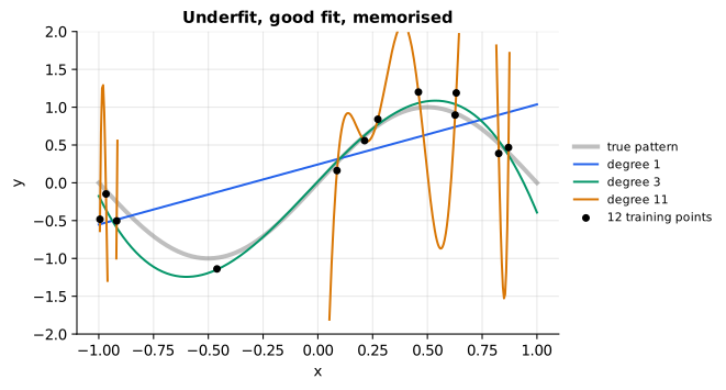
Reading it: the dots are 12 noisy samples of the grey sine curve (the true pattern). The straight line (degree 1) can't bend and misses the shape entirely: underfitting. The cubic (degree 3) follows the sine closely. The degree-11 polynomial passes through every dot exactly, and between and beyond them it swings wildly: it has memorised the noise.
The two numbers that tell these apart are errors on two different sets of data:
Level 3: the formula and its symbols
$$ \text{MSE}_{\text{train}} = \frac{1}{n}\sum_{i \in \text{train}} (y_i - \hat{y}_i)^2, \qquad \text{MSE}_{\text{val}} = \frac{1}{m}\sum_{j \in \text{val}} (y_j - \hat{y}_j)^2 $$
Symbols
| Symbol | Meaning here | In the example |
|---|---|---|
| $n, m$ | how many training and validation examples | 4 training points |
| $i \in \text{train}$ | "for every example $i$ in the training set" | $x = 0, 1, 2, 3$ |
| $y_i$ | the true value | 0, 1, 0, 1 |
| $\hat{y}_i$ | the model's prediction | 0.5 everywhere for the flat line |
| $\text{MSE}$ | mean squared error (see primer.ml.losses) |
0.25 for the flat line |
In words: "training error is the average squared miss on the data the model learned from; validation error is the same average on data it has never seen."
With the numbers: flat line: $\frac{1}{4}(0.5^2 + 0.5^2 + 0.5^2 + 0.5^2) = 0.25$. Cubic: every miss is 0, so training error is 0; its validation error on any point beyond x = 3 is enormous.
Level 3: in Python
In Python:
# the true values at x = 0, 1, 2, 3
y = [0, 1, 0, 1]
# the flat line predicts 0.5 everywhere
y_hat = [0.5, 0.5, 0.5, 0.5]
n = len(y)
# (1/n) Σ (y_i - ŷ_i)²
sum((y_i - y_hat_i) ** 2 for y_i, y_hat_i in zip(y, y_hat)) / n  # → 0.25
In code: zigzag_fit_error and zigzag_predict fit a polynomial of any
degree to the four zig-zag points and report its training error and its
prediction; true_function and make_curve_data draw the noisy sine
samples in the figure.
Why it matters: training error alone always rewards memorisation. The gap between training and validation error is the single most useful diagnostic in machine learning.
Underfitting vs. overfitting: finding the middle
Goldilocks tries three bowls of porridge: too cold, too hot, just right. Model capacity works the same way, and you find "just right" by measuring, not guessing: sweep the capacity and watch both errors.
Worked example: 12 noisy points from a sine wave, 300 fresh points for validation, polynomials of increasing degree.
| degree | training error | validation error | diagnosis |
|---|---|---|---|
| 1 | 0.20 | 0.30 | underfit: both high |
| 3 | 0.021 | 0.065 | about right |
| 5 | 0.013 | 0.057 | best: lowest validation error |
| 9 | 0.004 | 0.71 | overfit: validation 12× worse than at degree 5 |
| 11 | 0.0000 | 7,631 | memorised |
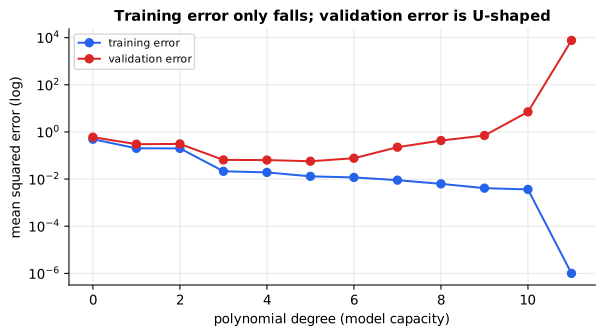
Reading it: the horizontal axis is model capacity (polynomial degree); the vertical axis is error on a log scale. The training curve (blue) only ever goes down: more capacity always fits the training data better. The validation curve (orange) falls, is nearly flat from degree 3 to 5 (lowest at 5), then climbs from degree 6 onward and shoots up. The left side of that valley is underfitting, the right side overfitting; the bottom is the model you want.
In code: polynomial_errors fits by least squares (choosing the
coefficients that minimise training MSE) and reports both errors.
Why it matters: "both errors high" and "training low, validation high" need opposite fixes. Underfitting wants more capacity, more features or more training; overfitting wants more data, regularization or early stopping. Diagnosing which one you have is the point.
Early stopping: take the cake out before it burns
A baker checks the cake with a toothpick every few minutes and takes it out when it comes out clean. Leave it longer and it burns, however good it was a minute ago. Training a flexible model is similar: validation error falls while the model learns the pattern, then rises once it starts memorising. Early stopping watches validation error during training, stops once it has failed to improve for a few checks (the patience), and keeps the weights from the best check.
Worked example: validation losses per epoch 1.0, 0.8, 0.6, 0.55, 0.58, 0.65, 0.7 with patience 2. Epoch 3 is the best. Epochs 4 and 5 are both worse, so training stops at epoch 5 and the weights from epoch 3 are kept.
flowchart LR
  E[End of epoch] --> V[Measure validation loss]
  V --> Q{Better than best?}
  Q -->|yes| S[Save weights,<br/>reset counter]
  Q -->|no| C[Counter + 1]
  C --> P{Counter = patience?}
  P -->|no| E2[Next epoch]
  P -->|yes| R[Stop; restore<br/>best weights]
  S --> E2
Reading it: after every epoch the loop asks one question: is this the best validation loss so far? If yes, snapshot the weights. If not, count a strike. Reaching the patience limit ends training and restores the snapshot, so you always ship the best model seen, not the last one.
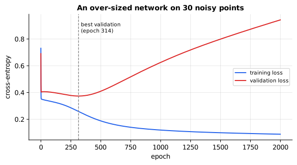
Reading it: a 64-unit network trained on only 30 noisy points. Both curves fall at first. Around epoch 300 (the dashed line) the validation curve bottoms out and turns upward while the training curve keeps falling: the network has started fitting individual noisy points. Everything to the right of the dashed line is wasted, or worse. Early stopping keeps the weights at the dashed line.
Level 3: the formula and its symbols
$$ t^\star = \arg\min_{t} \; \mathcal{L}_{\text{val}}(t), \qquad \text{stop at the first } t \text{ with } t - t^\star \ge \text{patience} $$
Symbols
| Symbol | Meaning here | In the example |
|---|---|---|
| $t$ | the epoch number | 0 to 6 |
| $\mathcal{L}_{\text{val}}(t)$ | validation loss after epoch $t$ | 0.55 at $t = 3$ |
| $\arg\min_t$ | "the $t$ at which the following is smallest" (the position, not the value) | 3 |
| $t^\star$ | "t-star", the best epoch so far | 3 |
| patience | how many non-improving epochs to tolerate | 2 |
In words: "remember the epoch with the lowest validation loss, and stop
once you've gone patience epochs past it without doing better."
With the numbers: $t^\star = 3$; at $t = 5$, $5 - 3 = 2 \ge 2$, so stop.
Level 3: in Python
In Python:
# validation loss after epoch t = 0, 1, 2, ...
L_val = [1.0, 0.8, 0.6, 0.55, 0.58, 0.65, 0.7]
patience = 2
t_star = 0
for t, loss in enumerate(L_val):
    if loss < L_val[t_star]:
        # a new best epoch: remember it
        t_star = t
    if t - t_star >= patience:
        # patience used up: stop here
        break
t_star, t  # → (3, 5)
In code: early_stopping replays a run's validation losses and returns
the best epoch and the epoch where training stops; train_flexible_model
trains the over-sized network in the figure and records both losses.
Why it matters: it's the cheapest regularizer there is: no change to the model, just a rule for when to stop. It's used almost everywhere a model is trained for multiple epochs, including fine-tuning language models.
Bias and variance: two ways to miss the target
Picture two archers. The first groups every arrow tightly, but a hand's width to the left of the bullseye: consistently wrong. That's bias. The second's arrows are centred on the bullseye on average but scattered all over the target: inconsistent. That's variance. A model trained on a different sample of data is like another volley of arrows. Simple models behave like the first archer; very flexible ones like the second.
Worked example: fit polynomials to 300 different random training sets of 30 points each, and measure (averaged over the input range):
| degree | bias² (systematic error) | variance (swing between training sets) |
|---|---|---|
| 1 | 0.174 | 0.022 |
| 3 | 0.0035 | 0.015 |
| 9 | 0.0038 | 4.5 |
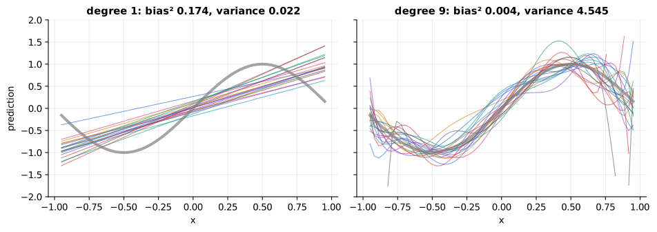
Reading it: each thin line is the model fitted to one random training set; the thick grey curve is the truth. On the left (degree 1), the lines agree with each other but all miss the sine's shape in the same way: high bias, low variance. On the right (degree 9), the lines follow the sine on average, but each one wiggles differently, especially near the edges: low bias, high variance.
Level 3: the formula and its symbols
$$ \mathbb{E}\big[(y - \hat{f}(x))^2\big] = \underbrace{\big(\mathbb{E}[\hat{f}(x)] - f(x)\big)^2}_{\text{bias}^2}
- \underbrace{\mathbb{E}\big[(\hat{f}(x) - \mathbb{E}[\hat{f}(x)])^2\big]}_{\text{variance}}
- \underbrace{\sigma^2}_{\text{noise}} $$
Symbols
| Symbol | Meaning here | In the example |
|---|---|---|
| $f(x)$ | the true pattern | $\sin(\pi x)$ |
| $\hat{f}(x)$ | "f-hat", the model's prediction, which depends on which training set it saw | one thin line |
| $\mathbb{E}[\cdot]$ | expected value: the average over many random training sets (and noise) | average of the 300 fits |
| $y$ | a noisy observation, $f(x)$ plus noise | |
| $\sigma^2$ | the noise variance: error no model can remove | $0.3^2 = 0.09$ |
In words: "a model's expected squared error on new data splits into how far its average prediction is from the truth (bias squared), plus how much its predictions scatter around their own average (variance), plus noise nobody can predict."
With the numbers: degree 1: $0.174 + 0.022 + 0.09 \approx 0.29$; degree 3: $0.0035 + 0.015 + 0.09 \approx 0.11$; degree 9: $0.0038 + 4.5 + 0.09 \approx 4.6$. Degree 3 has the best total.
Level 3: in Python
In Python:
sigma = 0.3
# σ²: the error no model can remove
noise = sigma ** 2
for degree, bias_sq, variance in [(1, 0.174, 0.022), (3, 0.0035, 0.015), (9, 0.0038, 4.5)]:
    # bias² + variance + σ²
    total = bias_sq + variance + noise
    # two significant figures
    print(degree, f"{total:.2g}")  # → 1 0.29 3 0.11 9 4.6
In code: bias_variance fits one polynomial to each of many random
training sets and splits their error into bias², variance and noise.
Why it matters: it names the two failure modes and explains why more data helps flexible models (averaging tames variance) but not rigid ones (more data doesn't fix bias). Very large neural networks complicate the picture ("double descent": past a point, even bigger models generalize better again), but the vocabulary is universal.
Dropout: nobody gets to be indispensable
A coach who randomly sends half the team home before each practice forces every player to learn every position; no single star can carry the team. Dropout does this to neurons: during training, each activation is set to zero with probability p on every step, so the network can't rely on any single neuron or fragile combination of neurons.
Worked example: four activations (1, 1, 1, 1), drop rate p = 0.5. Suppose the random mask keeps the last two: (0, 0, 1, 1). The survivors are scaled by 1 / (1 − 0.5) = 2, giving (0, 0, 2, 2). The average is still 1, so the next layer sees the same size signal on average. At evaluation time, nothing is dropped and nothing is scaled.
flowchart LR
  subgraph Train["Training step"]
    a1((1)) --> k1((0))
    a2((1)) --> k2((0))
    a3((1)) --> k3((2))
    a4((1)) --> k4((2))
  end
  subgraph Eval["Evaluation"]
    b1((1)) --> e1((1))
    b2((1)) --> e2((1))
    b3((1)) --> e3((1))
    b4((1)) --> e4((1))
  end
Reading it: on the left, one training step: two of the four units were dropped to 0 and the two survivors were doubled, so the total (4) matches what the full layer would have sent. A different random pair is dropped on the next step. On the right, at evaluation time every unit passes through unchanged. Scaling during training ("inverted dropout") is what lets evaluation be a plain pass-through.
$$ \tilde{h} = \frac{m \odot h}{1 - p}, \qquad m_i \sim \text{Bernoulli}(1 - p) $$
Symbols
| Symbol | Meaning here | In the example |
|---|---|---|
| $h$ | a layer's activations | (1, 1, 1, 1) |
| $\tilde{h}$ | "h-tilde", the activations after dropout | (0, 0, 2, 2) |
| $m$ | the random mask of 0s and 1s | (0, 0, 1, 1) |
| $m_i \sim \text{Bernoulli}(1-p)$ | each mask entry is independently 1 with probability $1 - p$, else 0 (a coin flip) | 50/50 |
| $p$ | the drop rate | 0.5 |
| $\odot$ | multiply entry by entry |
In words: "flip a biased coin for each activation, zero the ones that lose, and divide the survivors by the keep probability."
With the numbers: $(0\cdot1, 0\cdot1, 1\cdot1, 1\cdot1) / 0.5 = (0, 0, 2, 2)$.
Level 3: in Python
In Python:
import random
random.seed(0)
h = [1, 1, 1, 1]
p = 0.5
# m_i ~ Bernoulli(1 - p): a coin flip each
m = [1 if random.random() < 1 - p else 0 for _ in h]
m  # → [0, 0, 1, 1]
# (m ⊙ h) / (1 - p)
[m_i * h_i / (1 - p) for m_i, h_i in zip(m, h)]  # → [0.0, 0.0, 2.0, 2.0]
In code: dropout draws the mask and scales the survivors during
training, and passes activations through unchanged at evaluation time.
Why it matters: dropout was a key ingredient of the deep-learning
revival and is still used in many models (the original transformer used
p = 0.1). Forgetting to switch it off at evaluation (model.eval() in
PyTorch) is a classic bug that makes predictions noisy.
L1 and L2 penalties: a tax on large weights
Add a tax on the size of the weights to the loss, and the model must decide whether each weight earns its keep. L2 (ridge, "weight decay") taxes the square of each weight: big weights pay a lot, small ones almost nothing, so everything shrinks a little but nothing is eliminated. L1 (lasso) charges a flat rate per unit of size: small weights can't justify the fee, so they're wiped out entirely, to exactly zero.
Worked example: with independent (orthonormal) features, the penalized weights have a closed form. Start from the unpenalized weights (3, 0.5, −2) and use penalty strength 1:
| weight | L2: divide by 1 + 1 | L1: move 1 toward zero, stop at zero |
|---|---|---|
| 3 | 1.5 | 2 |
| 0.5 | 0.25 | 0 |
| −2 | −1 | −1 |
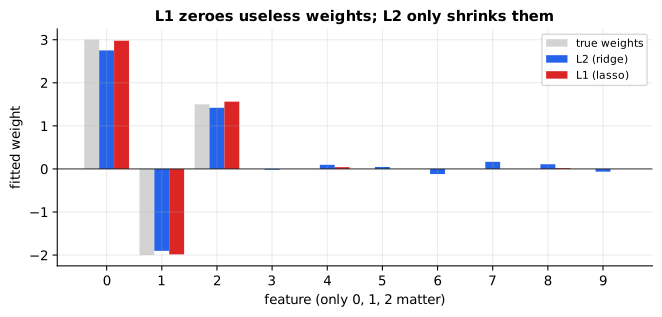
Reading it: ten features, but only the first three affect the target (grey bars show the true weights: 3, −2, 1.5, then zeros). The L2 fit (blue) shrinks everything a little and leaves small nonzero weights on all seven useless features. The L1 fit (orange) gets the three real weights nearly right and sets most of the useless ones to exactly zero: it has selected features for you.
Level 3: the formula and its symbols
$$ \text{L2: } \min_w \tfrac{1}{2}\lVert y - Xw \rVert^2 + \tfrac{\lambda}{2}\lVert w \rVert_2^2, \qquad \text{L1: } \min_w \tfrac{1}{2}\lVert y - Xw \rVert^2 + \lambda \lVert w \rVert_1 $$
Symbols
| Symbol | Meaning here | In the example |
|---|---|---|
| $\min_w$ | "choose the weights $w$ that make the following smallest" | |
| $X, y$ | the features (one row per example) and targets | |
| $\lVert y - Xw \rVert^2$ | the sum of squared prediction errors | |
| $\lambda$ | "lambda", the penalty strength | 1 |
| $\lVert w \rVert_2^2$ | the L2 norm squared: sum of squared weights | $3^2 + 0.5^2 + 2^2 = 13.25$ |
| $\lVert w \rVert_1$ | the L1 norm: sum of absolute weights | $3 + 0.5 + 2 = 5.5$ |
In words: "fit the data, but pay a penalty proportional to the sum of squared weights (L2) or the sum of absolute weights (L1)."
With the numbers: with orthonormal features the solutions are
$w_{\text{L2}} = w / (1 + \lambda) = (1.5, 0.25, -1)$ and
$w_{\text{L1}} = \text{sign}(w)\max(\lvert w \rvert - \lambda, 0) = (2, 0, -1)$,
the "soft threshold" in soft_threshold.
Level 3: in Python
In Python:
import math
w = [3, 0.5, -2]
# λ ("lambda" is taken in Python)
lam = 1
# ‖w‖₂², ‖w‖₁
sum(w_i ** 2 for w_i in w), sum(abs(w_i) for w_i in w)  # → (13.25, 5.5)
# L2: shrink every weight
[w_i / (1 + lam) for w_i in w]  # → [1.5, 0.25, -1.0]
# L1: sign(w) max(|w| - λ, 0)
[math.copysign(max(abs(w_i) - lam, 0), w_i) for w_i in w]  # → [2.0, 0.0, -1.0]
In code: penalised_weights gives both closed forms from the table, and
fit_sparse_problem fits the ten-feature problem in the figure (L1 by
alternating gradient steps with soft_threshold).
Why it matters: L2 (as weight decay; see AdamW in
primer.ml.optimizers) is on by default when training transformers. L1
is the tool when you want a sparse, interpretable model that uses only a
few features.
Train, validation and test: practice, mock and real exams
A student has practice questions (to learn from), a mock exam (to check progress and decide what to revise), and the real exam, sat once. Data is split the same way. Training data fits the weights. Validation data tunes choices like model size, learning rate and when to stop. Test data is touched once, at the end, to estimate real-world performance honestly. If you keep tuning against the test set, it quietly becomes a second validation set and stops being honest.
Worked example: 100 examples split 70 / 15 / 15, shuffled first, with no example in two sets. With only 10 examples, 5-fold cross-validation cuts them into 5 folds of 2; each fold takes a turn as the validation set while the model trains on the other 8, so every example is held out exactly once.
flowchart TB
  subgraph K["5-fold cross-validation"]
    f1["Run 1: [VAL] train train train train"]
    f2["Run 2: train [VAL] train train train"]
    f3["Run 3: train train [VAL] train train"]
    f4["Run 4: train train train [VAL] train"]
    f5["Run 5: train train train train [VAL]"]
  end
  K --> A[Average the 5 validation scores]
Reading it: the data is cut into five equal folds. In each run, one fold is held out (VAL) and the model is trained from scratch on the other four. Every example is validated on exactly once, and the average of the five scores is a steadier estimate than any single split.
Level 3: the formula and its symbols
$$ \text{CV score} = \frac{1}{k}\sum_{i=1}^{k} \text{score}\big(\text{model trained without fold } i,\ \text{fold } i\big) $$
Symbols
| Symbol | Meaning here | In the example |
|---|---|---|
| $k$ | number of folds | 5 |
| $i$ | which fold is held out | 1 to 5 |
| score(model, fold) | e.g. accuracy of that model on that fold |
In words: "train k models, each with one fold held out, and average their scores on the fold each one didn't see."
With the numbers: 10 examples, $k = 5$: five models, each trained on 8 and scored on 2; if they score 1.0, 0.5, 1.0, 1.0, 0.5, the CV score is 0.8.
Level 3: in Python
In Python:
examples = list(range(10))
k = 5
# 5 folds of 2
folds = [examples[2 * i: 2 * i + 2] for i in range(k)]
# each model trains on the other 8
[len(examples) - len(fold) for fold in folds]  # → [8, 8, 8, 8, 8]
# score of the model trained without fold i, on fold i
scores = [1.0, 0.5, 1.0, 1.0, 0.5]
# (1/k) Σ_i score_i
sum(scores) / k  # → 0.8
In code: train_val_test_split shuffles and cuts the indices into three
disjoint sets, and k_fold yields the training and validation indices for
each fold in turn.
Why it matters: with small datasets a single split is noisy, and cross-validation gives a more reliable estimate. With large datasets (or expensive models) one fixed validation set is enough.
Data leakage: the model saw the answers
A student who glimpsed the answer key scores perfectly on the practice exam and learns nothing. Data leakage is when information that won't be available at prediction time, or information from the test set, sneaks into training. Offline scores look superb; production scores collapse.
Worked examples:
- Duplicates across the split. Every row stored twice, labels 30% noisy (so no honest model can beat about 70%). Split before removing duplicates, and a model that just copies its nearest training row scores 87%: it's reading the answers off each test row's twin. Deduplicate first and the same model scores about 50%.
- A feature from the future. A fraud model is given
chargeback_filed, a column filled in only after a customer disputes a charge, which is to say after the outcome. Offline accuracy: 98%. In production that column is always empty at decision time, and accuracy falls to 49%, worse than an honest model using only the legitimate features (61%).
flowchart LR
  subgraph T["Timeline of one transaction"]
    direction LR
    A[Transaction happens] --> P["Model must decide<br/>(prediction time)"]
    P --> O[Fraud confirmed?]
    O --> C[chargeback_filed recorded]
  end
  C -. "leaks backwards into<br/>the training table" .-> P
Reading it: read the timeline left to right. The model has to decide at the second box. The chargeback is only recorded at the last box, after the outcome is known. In a historical training table every column sits side by side, so nothing stops the model from using a column that, in real time, it could never have had. The dotted arrow is the leak.
In code: duplicate_leakage_demo and future_feature_demo run both
examples; the "model" in the first is a one-nearest-neighbour lookup (copy the label
of the closest training row), the purest memoriser there is.
Why it matters: leakage is the most common reason a model that looked great in evaluation fails in production. For language-model benchmarks the big version is contamination: test questions that appeared in the pretraining data. The defences are procedural: deduplicate before splitting, split by time or by user when the real task is predicting the future or new users, and ask of every feature "would I actually know this at prediction time?"
In 20 seconds
- Overfitting: training error falls while validation error rises; the model memorised noise. Underfitting: both errors are high.
- Fixes for overfitting: more data, early stopping, dropout, weight decay (L2), L1 for sparsity, data augmentation.
- Bias is systematic error (too simple); variance is sensitivity to the training sample (too flexible).
- Train fits weights, validation tunes choices, test is touched once; cross-validation for small data.
- Leakage (duplicates across splits, features from the future) gives great offline scores that collapse in production.
Self-test questions
Training loss drops while validation loss rises. What's happening, and what helps? Overfitting: the model is memorising training-set noise. Stop early (keep the best-validation weights), add regularization (dropout, weight decay), get more or more varied data, or reduce capacity.
How do you tell underfitting from overfitting? Underfitting: training and validation errors are both high. Overfitting: training error is low and validation error is much higher. They need opposite fixes.
Why does dropout scale the surviving activations by 1/(1 − p)? So the expected value of each activation is the same during training as at evaluation, where nothing is dropped. The evaluation-time network can then be used as is.
Why does L1 produce exact zeros but L2 doesn't? L1's penalty has a constant slope, so small weights feel a fixed pull toward zero that the data can't outweigh; they're thresholded to zero. L2's pull is proportional to the weight, so it fades as a weight shrinks and never quite reaches zero.
Why must the test set be touched only once? Every decision made by looking at test scores fits the model to the test set a little. Do it repeatedly and the test score stops being an unbiased estimate of performance on new data.
Give two examples of data leakage. The same (or near-duplicate) documents in both the training and test splits; and a feature that's only known after the outcome (a chargeback flag in a fraud model). For LLM evaluation: benchmark questions present in the pretraining data.
The papers behind this lesson
- Srivastava, Hinton, Krizhevsky, Sutskever & Salakhutdinov, Dropout: A Simple Way to Prevent Neural Networks from Overfitting (JMLR, 2014): https://jmlr.org/papers/v15/srivastava14a.html Introduced dropout and showed it as a cheap approximation to averaging many networks. annotated companion
- Tibshirani, Regression Shrinkage and Selection via the Lasso (JRSS B, 1996): https://www.jstor.org/stable/2346178 Introduced the L1 penalty and its property of setting coefficients exactly to zero.
- Geman, Bienenstock & Doursat, Neural Networks and the Bias/Variance Dilemma (Neural Computation, 1992): https://doi.org/10.1162/neco.1992.4.1.1 Framed generalization in neural networks as the bias-variance trade-off.
- Belkin, Hsu, Ma & Mandal, Reconciling modern machine learning practice and the bias-variance trade-off (2018): https://arxiv.org/abs/1812.11118 Documented "double descent", where very over-parameterized models generalize better again.
- Kapoor & Narayanan, Leakage and the Reproducibility Crisis in ML-based Science (2022): https://arxiv.org/abs/2207.07048 Catalogued the kinds of data leakage and how widely they inflate published results.
Further reading
- Goodfellow, Bengio & Courville, Deep Learning, ch. 7 (regularization): https://www.deeplearningbook.org/contents/regularization.html
- CS231n notes, Neural Networks Part 2 (regularization and dropout): https://cs231n.github.io/neural-networks-2/
- Hastie, Tibshirani & Friedman, The Elements of Statistical Learning (free PDF; ch. 3 and 7): https://hastie.su.domains/ElemStatLearn/
- scikit-learn user guide, Cross-validation: https://scikit-learn.org/stable/modules/cross_validation.html
1r""" 2# Regularization: learning the pattern instead of memorising the examples 3 4Run: `python -m primer.ml.regularization` 5 6New to the notation? `primer.notation` explains every symbol used here from 7zero. This lesson builds on the losses in `primer.ml.losses` and the 8training loop in `primer.ml.neural_net`. 9 10## Level 1: The practitioner's guide 11 12**In one sentence.** Regularization is everything you do to make a model 13learn the pattern in its training data rather than memorise the examples, 14and the way you know it is working is the gap between the error on data 15the model trained on and the error on data it has never seen. 16 17**When you need it.** Whenever you train or fine-tune anything on less data 18than the model could memorise, which in practice is always: a fine-tune on 19a few thousand examples, a classifier on a table of ten thousand rows, a 20forecasting model on a year of history. The tell is a training error that 21keeps falling while the validation error turns and climbs. This lesson's 22polynomial sweep shows the whole story in one table: at degree 5 the 23training error is 0.013 and the validation error 0.057; at degree 9 the 24training error has dropped to 0.004 and the validation error has risen 25twelve-fold to 0.71; at degree 11 the training error is zero and the 26validation error is 7,631. Its over-sized network bottoms out on 27validation near epoch 300 and gets steadily worse for the next 1,700 28epochs while its training loss keeps improving. The other tell is the 29opposite one, and it hides in a good offline score: a model that looked 30superb in evaluation and collapsed in production has usually seen the 31answers, and that is leakage, which the same lesson covers. You do not need 32more regularization when both errors are high; that is underfitting, and it 33wants more capacity, more features or more training, the opposite fix. 34 35**Your options.** From the cheapest to the most involved: 36 37| Option | What it does | What it guarantees | What it costs | Where it lives | 38|---|---|---|---|---| 39| A held-out validation set (and a test set touched once) | Measures the gap that every other option is judged by | An honest estimate, as long as the test set is not used to choose | 15% to 30% of your data, and discipline | Your data pipeline | 40| Early stopping | Watches validation loss, stops after `patience` bad checks, restores the best weights | You ship the best model seen, not the last | A validation pass per epoch; nothing in the model | The training loop: a callback in every framework | 41| More data, or augmented data | Averages the noise away | Tames variance in flexible models; does nothing for a model too simple to fit the pattern | Collection or labelling time | Your data | 42| L2 penalty (weight decay) | Taxes the square of every weight, so all of them shrink a little | Smaller, smoother weights; nothing is eliminated | One hyperparameter, λ | The optimiser: on by default in AdamW | 43| Dropout | Zeroes each activation with probability p on every training step, scaled so evaluation is a plain pass-through | No neuron becomes indispensable | Slower convergence; a bug if left on at evaluation | The model, between layers | 44| L1 penalty (lasso) | Charges a flat fee per unit of weight, so small weights go to exactly zero | A sparse model that names its features | Harder optimisation; one hyperparameter | Linear and tabular models, feature selection | 45| Less capacity | A smaller model, a lower polynomial degree, fewer features | Less to memorise with | Possibly too little to learn the pattern | The architecture | 46| Cross-validation | Trains k models, each with one fold held out, and averages their scores | A steadier estimate than one split when data is small | k training runs | Small tabular problems; scikit-learn's cross-validation guide | 47| Leak-proof splitting | Deduplicates before splitting, splits by time or by user, drops features unknown at prediction time | An offline score that survives production | Thinking about the timeline of every feature | Your data pipeline, before any training | 48 49**How to choose.** Diagnose first, because the two failures want opposite 50cures. 51 52- Both errors high: underfitting. Add capacity, features or training time. 53 Regularizing further makes it worse. 54- Training low, validation high: overfitting. Early stopping first, because 55 it costs nothing; then weight decay (which you probably already have) and 56 dropout; then more data if you can get it. 57- A tabular model you must explain, or hundreds of features of which a few 58 matter: L1, which in this lesson zeroes 5 of 7 useless weights while L2 59 zeroes none. 60- Fewer than a few thousand examples: cross-validate rather than trust one 61 split. 62- A model that was wonderful offline: before celebrating, check for twins 63 across the split and for columns filled in after the outcome. 64- Whatever you pick, the test set is touched once, at the end. Every 65 decision made by looking at it turns it into a second validation set, and 66 the benchmark version of this failure is Goodhart's law in 67 `primer.ml.benchmarks`. 68 69**What it costs.** Early stopping costs one validation pass per epoch and 70stops training sooner, so it usually saves compute. Weight decay and L1 cost 71nothing at inference and one hyperparameter each; PyTorch's AdamW defaults 72weight decay to 0.01. Dropout slows training, because each step trains a 73thinned network, and the original transformer used p = 0.1 rather than 74anything heavier. Cross-validation multiplies training cost by the number 75of folds. The dear cost is data: the validation and test sets are examples 76you cannot train on, and with 100 examples a 70 / 15 / 15 split leaves 15 77for each. Leakage costs the most of all, late: this lesson's fraud model 78with a future feature scores 98% offline and 49% in production, worse than 79the honest model's 61%. 80 81**What breaks.** 82 83- **Dropout left on at evaluation.** Predictions become noisy and change 84 from call to call. Switch the model to evaluation mode; the lesson's 85 `dropout` passes activations through unchanged there. 86- **Early stopping with no restore.** Stopping is half the job; the weights 87 at the stop are the ones that just failed twice. Keep the snapshot from 88 the best check. 89- **Patience too short.** A noisy validation curve stops training on a 90 blip. Smooth it, or raise the patience. 91- **Tuning against the test set.** Each look fits the model to it a little. 92 Choose with validation, report with test. 93- **Duplicates across the split.** A nearest-neighbour memoriser scores 87% 94 on data whose labels are 30% noise, when no honest model can beat about 95 70%; deduplicated, it scores 50%. Deduplicate before splitting. 96- **A feature from the future.** `chargeback_filed` is recorded after the 97 outcome. Ask of every column: would I know this at prediction time? 98- **A random split on time-ordered data.** Predicting next month from a 99 shuffle of all months is a leak. Split by time when the task is the 100 future, by user when the task is new users. 101- **Regularizing an underfit model.** It cannot get better by learning 102 less. Look at both curves before reaching for the penalty. 103 104**In the wild.** Weight decay is on by default in the optimisers that train 105transformers: `torch.optim.AdamW` takes `weight_decay` with a default of 1060.01, and `primer.ml.optimizers` shows why decoupling it from the gradient 107step mattered. Early stopping is a callback everywhere it is offered; 108Keras's `EarlyStopping` has `patience` and `restore_best_weights`, which 109default to 0 and False, so a naive call gets neither. Dropout (Srivastava 110et al., 2014) trains at p = 0.1 in the original transformer and is switched 111off by `model.eval()` in PyTorch. The lasso is Tibshirani (1996), and 112scikit-learn's cross-validation guide is the standard reference for folds 113that respect groups and time. Kapoor and Narayanan (2022) catalogued the 114kinds of leakage and how widely they inflate published results, and Belkin 115et al. (2018) documented double descent, where very over-parameterised 116models generalise well again, which is why the modern recipe is a large 117model plus regularization rather than a small model. 118 119**Go deeper.** Level 2 fits the memorising cubic by hand, sweeps polynomial 120degree to draw the valley in validation error, replays early stopping on a 121list of losses, splits error into bias and variance over 300 training sets, 122builds dropout and the two penalties in a few lines each, cuts data into 123folds, and reproduces both leaks with a nearest-neighbour memoriser. If you 124only needed to diagnose a curve and pick a fix, you are done. 125 126## Level 2: How it works, from scratch 127 128Two students prepare for an exam. One learns the ideas. The other memorises 129last year's paper, answer by answer, and scores 100% on it in practice. On 130the real exam, with new questions, the first student does fine and the 131second falls apart. A model that memorises its training examples, noise 132and all, instead of learning the pattern behind them is **overfitting**. It 133looks brilliant on the data it has seen and fails on data it hasn't. 134**Regularization** is everything we do to push a model toward the first 135student. 136 137Worked example: four training points (0, 0), (1, 1), (2, 0), (3, 1), a 138zig-zag that is really "about 0.5, plus noise". 139 140| model | error on the 4 training points | prediction at x = 4 | 141|---|---|---| 142| flat line at 0.5 (the pattern) | 0.25 | 0.5 | 143| cubic through all four points (memorised) | **0** | **8** | 144 145The cubic is perfect on the training data and absurd one step beyond it. 146You can check the 8 by hand with a difference table: the values 0, 1, 0, 1 147have differences 1, −1, 1, then −2, 2, then 4; a cubic keeps that last 148difference constant, so extending the table gives 6, then 7, then 8. 149 150```mermaid 151flowchart LR 152 D["Training data =<br/>pattern + noise"] --> M{Model capacity} 153 M -->|too little| U["Underfits:<br/>misses the pattern"] 154 M -->|about right| G["Generalizes:<br/>learns the pattern"] 155 M -->|too much, unchecked| O["Overfits:<br/>memorises the noise"] 156 G --> N[Good on new data] 157 U & O --> B[Bad on new data] 158``` 159 160**Reading it:** every dataset is a pattern plus noise. A model with too 161little capacity can't even represent the pattern; one with too much, left 162unchecked, fits the noise too. Only the middle path does well on new data. 163Regularization techniques are ways of steering a high-capacity model onto 164that middle path without giving up its capacity. 165 166 167 168**Reading it:** the dots are 12 noisy samples of the grey sine curve (the 169true pattern). The straight line (degree 1) can't bend and misses the shape 170entirely: underfitting. The cubic (degree 3) follows the sine closely. The 171degree-11 polynomial passes through every dot exactly, and between and 172beyond them it swings wildly: it has memorised the noise. 173 174The two numbers that tell these apart are errors on two different sets of 175data: 176 177$$ 178\text{MSE}_{\text{train}} = \frac{1}{n}\sum_{i \in \text{train}} (y_i - \hat{y}_i)^2, 179\qquad 180\text{MSE}_{\text{val}} = \frac{1}{m}\sum_{j \in \text{val}} (y_j - \hat{y}_j)^2 181$$ 182 183**Symbols** 184 185| Symbol | Meaning here | In the example | 186|---|---|---| 187| $n, m$ | how many training and validation examples | 4 training points | 188| $i \in \text{train}$ | "for every example $i$ in the training set" | $x = 0, 1, 2, 3$ | 189| $y_i$ | the true value | 0, 1, 0, 1 | 190| $\hat{y}_i$ | the model's prediction | 0.5 everywhere for the flat line | 191| $\text{MSE}$ | mean squared error (see `primer.ml.losses`) | 0.25 for the flat line | 192 193**In words:** "training error is the average squared miss on the data the 194model learned from; validation error is the same average on data it has 195never seen." 196 197**With the numbers:** flat line: $\frac{1}{4}(0.5^2 + 0.5^2 + 0.5^2 + 0.5^2) = 0.25$. 198Cubic: every miss is 0, so training error is 0; its validation error on any 199point beyond x = 3 is enormous. 200 201**In Python:** 202 203```python 204# the true values at x = 0, 1, 2, 3 205y = [0, 1, 0, 1] 206# the flat line predicts 0.5 everywhere 207y_hat = [0.5, 0.5, 0.5, 0.5] 208n = len(y) 209# (1/n) Σ (y_i - ŷ_i)² 210sum((y_i - y_hat_i) ** 2 for y_i, y_hat_i in zip(y, y_hat)) / n # → 0.25 211``` 212 213**In code:** `zigzag_fit_error` and `zigzag_predict` fit a polynomial of any 214degree to the four zig-zag points and report its training error and its 215prediction; `true_function` and `make_curve_data` draw the noisy sine 216samples in the figure. 217 218**Why it matters:** training error alone always rewards memorisation. The 219gap between training and validation error is the single most useful 220diagnostic in machine learning. 221 222## Underfitting vs. overfitting: finding the middle 223 224Goldilocks tries three bowls of porridge: too cold, too hot, just right. 225Model capacity works the same way, and you find "just right" by measuring, 226not guessing: sweep the capacity and watch both errors. 227 228Worked example: 12 noisy points from a sine wave, 300 fresh points for 229validation, polynomials of increasing degree. 230 231| degree | training error | validation error | diagnosis | 232|---|---|---|---| 233| 1 | 0.20 | 0.30 | underfit: both high | 234| 3 | 0.021 | 0.065 | about right | 235| 5 | 0.013 | 0.057 | best: lowest validation error | 236| 9 | 0.004 | 0.71 | overfit: validation 12× worse than at degree 5 | 237| 11 | 0.0000 | 7,631 | memorised | 238 239 240 241**Reading it:** the horizontal axis is model capacity (polynomial degree); 242the vertical axis is error on a log scale. The training curve (blue) only 243ever goes down: more capacity always fits the training data better. The 244validation curve (orange) falls, is nearly flat from degree 3 to 5 (lowest 245at 5), then climbs from degree 6 onward and shoots up. The left side of that valley is underfitting, the right side 246overfitting; the bottom is the model you want. 247 248**In code:** `polynomial_errors` fits by least squares (choosing the 249coefficients that minimise training MSE) and reports both errors. 250 251**Why it matters:** "both errors high" and "training low, validation high" 252need opposite fixes. Underfitting wants more capacity, more features or more 253training; overfitting wants more data, regularization or early stopping. 254Diagnosing which one you have is the point. 255 256## Early stopping: take the cake out before it burns 257 258A baker checks the cake with a toothpick every few minutes and takes it out 259when it comes out clean. Leave it longer and it burns, however good it was 260a minute ago. Training a flexible model is similar: validation error falls 261while the model learns the pattern, then rises once it starts memorising. 262**Early stopping** watches validation error during training, stops once it 263has failed to improve for a few checks (the **patience**), and keeps the 264weights from the best check. 265 266Worked example: validation losses per epoch 1.0, 0.8, 0.6, **0.55**, 0.58, 2670.65, 0.7 with patience 2. Epoch 3 is the best. Epochs 4 and 5 are both 268worse, so training stops at epoch 5 and the weights from epoch 3 are kept. 269 270```mermaid 271flowchart LR 272 E[End of epoch] --> V[Measure validation loss] 273 V --> Q{Better than best?} 274 Q -->|yes| S[Save weights,<br/>reset counter] 275 Q -->|no| C[Counter + 1] 276 C --> P{Counter = patience?} 277 P -->|no| E2[Next epoch] 278 P -->|yes| R[Stop; restore<br/>best weights] 279 S --> E2 280``` 281 282**Reading it:** after every epoch the loop asks one question: is this the 283best validation loss so far? If yes, snapshot the weights. If not, count a 284strike. Reaching the patience limit ends training and restores the 285snapshot, so you always ship the best model seen, not the last one. 286 287 288 289**Reading it:** a 64-unit network trained on only 30 noisy points. Both 290curves fall at first. Around epoch 300 (the dashed line) the validation 291curve bottoms out and turns upward while the training curve keeps falling: 292the network has started fitting individual noisy points. Everything to the 293right of the dashed line is wasted, or worse. Early stopping keeps the 294weights at the dashed line. 295 296$$ 297t^\star = \arg\min_{t} \; \mathcal{L}_{\text{val}}(t), 298\qquad \text{stop at the first } t \text{ with } t - t^\star \ge \text{patience} 299$$ 300 301**Symbols** 302 303| Symbol | Meaning here | In the example | 304|---|---|---| 305| $t$ | the epoch number | 0 to 6 | 306| $\mathcal{L}_{\text{val}}(t)$ | validation loss after epoch $t$ | 0.55 at $t = 3$ | 307| $\arg\min_t$ | "the $t$ at which the following is smallest" (the position, not the value) | 3 | 308| $t^\star$ | "t-star", the best epoch so far | 3 | 309| patience | how many non-improving epochs to tolerate | 2 | 310 311**In words:** "remember the epoch with the lowest validation loss, and stop 312once you've gone `patience` epochs past it without doing better." 313 314**With the numbers:** $t^\star = 3$; at $t = 5$, $5 - 3 = 2 \ge 2$, so stop. 315 316**In Python:** 317 318```python 319# validation loss after epoch t = 0, 1, 2, ... 320L_val = [1.0, 0.8, 0.6, 0.55, 0.58, 0.65, 0.7] 321patience = 2 322t_star = 0 323for t, loss in enumerate(L_val): 324 if loss < L_val[t_star]: 325 # a new best epoch: remember it 326 t_star = t 327 if t - t_star >= patience: 328 # patience used up: stop here 329 break 330t_star, t # → (3, 5) 331``` 332 333**In code:** `early_stopping` replays a run's validation losses and returns 334the best epoch and the epoch where training stops; `train_flexible_model` 335trains the over-sized network in the figure and records both losses. 336 337**Why it matters:** it's the cheapest regularizer there is: no change to the 338model, just a rule for when to stop. It's used almost everywhere a model is 339trained for multiple epochs, including fine-tuning language models. 340 341## Bias and variance: two ways to miss the target 342 343Picture two archers. The first groups every arrow tightly, but a hand's 344width to the left of the bullseye: consistently wrong. That's **bias**. The 345second's arrows are centred on the bullseye on average but scattered all 346over the target: inconsistent. That's **variance**. A model trained on a 347different sample of data is like another volley of arrows. Simple models 348behave like the first archer; very flexible ones like the second. 349 350Worked example: fit polynomials to 300 different random training sets of 30 351points each, and measure (averaged over the input range): 352 353| degree | bias² (systematic error) | variance (swing between training sets) | 354|---|---|---| 355| 1 | 0.174 | 0.022 | 356| 3 | 0.0035 | 0.015 | 357| 9 | 0.0038 | 4.5 | 358 359 360 361**Reading it:** each thin line is the model fitted to one random training 362set; the thick grey curve is the truth. On the left (degree 1), the lines 363agree with each other but all miss the sine's shape in the same way: high 364bias, low variance. On the right (degree 9), the lines follow the sine on 365average, but each one wiggles differently, especially near the edges: low 366bias, high variance. 367 368$$ 369\mathbb{E}\big[(y - \hat{f}(x))^2\big] = \underbrace{\big(\mathbb{E}[\hat{f}(x)] - f(x)\big)^2}_{\text{bias}^2} 370+ \underbrace{\mathbb{E}\big[(\hat{f}(x) - \mathbb{E}[\hat{f}(x)])^2\big]}_{\text{variance}} 371+ \underbrace{\sigma^2}_{\text{noise}} 372$$ 373 374**Symbols** 375 376| Symbol | Meaning here | In the example | 377|---|---|---| 378| $f(x)$ | the true pattern | $\sin(\pi x)$ | 379| $\hat{f}(x)$ | "f-hat", the model's prediction, which depends on which training set it saw | one thin line | 380| $\mathbb{E}[\cdot]$ | expected value: the average over many random training sets (and noise) | average of the 300 fits | 381| $y$ | a noisy observation, $f(x)$ plus noise | | 382| $\sigma^2$ | the noise variance: error no model can remove | $0.3^2 = 0.09$ | 383 384**In words:** "a model's expected squared error on new data splits into how 385far its average prediction is from the truth (bias squared), plus how much 386its predictions scatter around their own average (variance), plus noise 387nobody can predict." 388 389**With the numbers:** degree 1: $0.174 + 0.022 + 0.09 \approx 0.29$; 390degree 3: $0.0035 + 0.015 + 0.09 \approx 0.11$; degree 9: 391$0.0038 + 4.5 + 0.09 \approx 4.6$. Degree 3 has the best total. 392 393**In Python:** 394 395```python 396sigma = 0.3 397# σ²: the error no model can remove 398noise = sigma ** 2 399for degree, bias_sq, variance in [(1, 0.174, 0.022), (3, 0.0035, 0.015), (9, 0.0038, 4.5)]: 400 # bias² + variance + σ² 401 total = bias_sq + variance + noise 402 # two significant figures 403 print(degree, f"{total:.2g}") # → 1 0.29 3 0.11 9 4.6 404``` 405 406**In code:** `bias_variance` fits one polynomial to each of many random 407training sets and splits their error into bias², variance and noise. 408 409**Why it matters:** it names the two failure modes and explains why more 410data helps flexible models (averaging tames variance) but not rigid ones 411(more data doesn't fix bias). Very large neural networks complicate the 412picture ("double descent": past a point, even bigger models generalize 413better again), but the vocabulary is universal. 414 415## Dropout: nobody gets to be indispensable 416 417A coach who randomly sends half the team home before each practice forces 418every player to learn every position; no single star can carry the team. 419**Dropout** does this to neurons: during training, each activation is set 420to zero with probability p on every step, so the network can't rely on any 421single neuron or fragile combination of neurons. 422 423Worked example: four activations (1, 1, 1, 1), drop rate p = 0.5. Suppose 424the random mask keeps the last two: (0, 0, 1, 1). The survivors are scaled by 4251 / (1 − 0.5) = 2, giving (0, 0, 2, 2). The average is still 1, so the next 426layer sees the same size signal on average. At evaluation time, nothing is 427dropped and nothing is scaled. 428 429```mermaid 430flowchart LR 431 subgraph Train["Training step"] 432 a1((1)) --> k1((0)) 433 a2((1)) --> k2((0)) 434 a3((1)) --> k3((2)) 435 a4((1)) --> k4((2)) 436 end 437 subgraph Eval["Evaluation"] 438 b1((1)) --> e1((1)) 439 b2((1)) --> e2((1)) 440 b3((1)) --> e3((1)) 441 b4((1)) --> e4((1)) 442 end 443``` 444 445**Reading it:** on the left, one training step: two of the four units were 446dropped to 0 and the two survivors were doubled, so the total (4) matches 447what the full layer would have sent. A different random pair is dropped on 448the next step. On the right, at evaluation time every unit passes through 449unchanged. Scaling during training ("inverted dropout") is what lets 450evaluation be a plain pass-through. 451 452$$ 453\tilde{h} = \frac{m \odot h}{1 - p}, \qquad m_i \sim \text{Bernoulli}(1 - p) 454$$ 455 456**Symbols** 457 458| Symbol | Meaning here | In the example | 459|---|---|---| 460| $h$ | a layer's activations | (1, 1, 1, 1) | 461| $\tilde{h}$ | "h-tilde", the activations after dropout | (0, 0, 2, 2) | 462| $m$ | the random mask of 0s and 1s | (0, 0, 1, 1) | 463| $m_i \sim \text{Bernoulli}(1-p)$ | each mask entry is independently 1 with probability $1 - p$, else 0 (a coin flip) | 50/50 | 464| $p$ | the drop rate | 0.5 | 465| $\odot$ | multiply entry by entry | | 466 467**In words:** "flip a biased coin for each activation, zero the ones that 468lose, and divide the survivors by the keep probability." 469 470**With the numbers:** $(0\cdot1, 0\cdot1, 1\cdot1, 1\cdot1) / 0.5 = (0, 0, 2, 2)$. 471 472**In Python:** 473 474```python 475import random 476random.seed(0) 477h = [1, 1, 1, 1] 478p = 0.5 479# m_i ~ Bernoulli(1 - p): a coin flip each 480m = [1 if random.random() < 1 - p else 0 for _ in h] 481m # → [0, 0, 1, 1] 482# (m ⊙ h) / (1 - p) 483[m_i * h_i / (1 - p) for m_i, h_i in zip(m, h)] # → [0.0, 0.0, 2.0, 2.0] 484``` 485 486**In code:** `dropout` draws the mask and scales the survivors during 487training, and passes activations through unchanged at evaluation time. 488 489**Why it matters:** dropout was a key ingredient of the deep-learning 490revival and is still used in many models (the original transformer used 491p = 0.1). Forgetting to switch it off at evaluation (`model.eval()` in 492PyTorch) is a classic bug that makes predictions noisy. 493 494## L1 and L2 penalties: a tax on large weights 495 496Add a tax on the size of the weights to the loss, and the model must decide 497whether each weight earns its keep. **L2** (ridge, "weight decay") taxes the 498*square* of each weight: big weights pay a lot, small ones almost nothing, 499so everything shrinks a little but nothing is eliminated. **L1** (lasso) 500charges a flat rate per unit of size: small weights can't justify the 501fee, so they're wiped out entirely, to exactly zero. 502 503Worked example: with independent (orthonormal) features, the penalized 504weights have a closed form. Start from the unpenalized weights (3, 0.5, −2) 505and use penalty strength 1: 506 507| weight | L2: divide by 1 + 1 | L1: move 1 toward zero, stop at zero | 508|---|---|---| 509| 3 | 1.5 | 2 | 510| 0.5 | 0.25 | **0** | 511| −2 | −1 | −1 | 512 513 514 515**Reading it:** ten features, but only the first three affect the target 516(grey bars show the true weights: 3, −2, 1.5, then zeros). The L2 fit (blue) 517shrinks everything a little and leaves small nonzero weights on all seven 518useless features. The L1 fit (orange) gets the three real weights nearly 519right and sets most of the useless ones to exactly zero: it has selected 520features for you. 521 522$$ 523\text{L2: } \min_w \tfrac{1}{2}\lVert y - Xw \rVert^2 + \tfrac{\lambda}{2}\lVert w \rVert_2^2, 524\qquad 525\text{L1: } \min_w \tfrac{1}{2}\lVert y - Xw \rVert^2 + \lambda \lVert w \rVert_1 526$$ 527 528**Symbols** 529 530| Symbol | Meaning here | In the example | 531|---|---|---| 532| $\min_w$ | "choose the weights $w$ that make the following smallest" | | 533| $X, y$ | the features (one row per example) and targets | | 534| $\lVert y - Xw \rVert^2$ | the sum of squared prediction errors | | 535| $\lambda$ | "lambda", the penalty strength | 1 | 536| $\lVert w \rVert_2^2$ | the L2 norm squared: sum of squared weights | $3^2 + 0.5^2 + 2^2 = 13.25$ | 537| $\lVert w \rVert_1$ | the L1 norm: sum of absolute weights | $3 + 0.5 + 2 = 5.5$ | 538 539**In words:** "fit the data, but pay a penalty proportional to the sum of 540squared weights (L2) or the sum of absolute weights (L1)." 541 542**With the numbers:** with orthonormal features the solutions are 543$w_{\text{L2}} = w / (1 + \lambda) = (1.5, 0.25, -1)$ and 544$w_{\text{L1}} = \text{sign}(w)\max(\lvert w \rvert - \lambda, 0) = (2, 0, -1)$, 545the "soft threshold" in `soft_threshold`. 546 547**In Python:** 548 549```python 550import math 551w = [3, 0.5, -2] 552# λ ("lambda" is taken in Python) 553lam = 1 554# ‖w‖₂², ‖w‖₁ 555sum(w_i ** 2 for w_i in w), sum(abs(w_i) for w_i in w) # → (13.25, 5.5) 556# L2: shrink every weight 557[w_i / (1 + lam) for w_i in w] # → [1.5, 0.25, -1.0] 558# L1: sign(w) max(|w| - λ, 0) 559[math.copysign(max(abs(w_i) - lam, 0), w_i) for w_i in w] # → [2.0, 0.0, -1.0] 560``` 561 562**In code:** `penalised_weights` gives both closed forms from the table, and 563`fit_sparse_problem` fits the ten-feature problem in the figure (L1 by 564alternating gradient steps with `soft_threshold`). 565 566**Why it matters:** L2 (as weight decay; see AdamW in 567`primer.ml.optimizers`) is on by default when training transformers. L1 568is the tool when you want a sparse, interpretable model that uses only a 569few features. 570 571## Train, validation and test: practice, mock and real exams 572 573A student has practice questions (to learn from), a mock exam (to check 574progress and decide what to revise), and the real exam, sat once. Data is 575split the same way. **Training data** fits the weights. **Validation data** 576tunes choices like model size, learning rate and when to stop. **Test data** 577is touched once, at the end, to estimate real-world performance honestly. 578If you keep tuning against the test set, it quietly becomes a second 579validation set and stops being honest. 580 581Worked example: 100 examples split 70 / 15 / 15, shuffled first, with no 582example in two sets. With only 10 examples, **5-fold cross-validation** cuts 583them into 5 folds of 2; each fold takes a turn as the validation set while 584the model trains on the other 8, so every example is held out exactly once. 585 586```mermaid 587flowchart TB 588 subgraph K["5-fold cross-validation"] 589 f1["Run 1: [VAL] train train train train"] 590 f2["Run 2: train [VAL] train train train"] 591 f3["Run 3: train train [VAL] train train"] 592 f4["Run 4: train train train [VAL] train"] 593 f5["Run 5: train train train train [VAL]"] 594 end 595 K --> A[Average the 5 validation scores] 596``` 597 598**Reading it:** the data is cut into five equal folds. In each run, one fold 599is held out (VAL) and the model is trained from scratch on the other four. 600Every example is validated on exactly once, and the average of the five 601scores is a steadier estimate than any single split. 602 603$$ 604\text{CV score} = \frac{1}{k}\sum_{i=1}^{k} \text{score}\big(\text{model trained without fold } i,\ \text{fold } i\big) 605$$ 606 607**Symbols** 608 609| Symbol | Meaning here | In the example | 610|---|---|---| 611| $k$ | number of folds | 5 | 612| $i$ | which fold is held out | 1 to 5 | 613| score(model, fold) | e.g. accuracy of that model on that fold | | 614 615**In words:** "train k models, each with one fold held out, and average 616their scores on the fold each one didn't see." 617 618**With the numbers:** 10 examples, $k = 5$: five models, each trained on 8 619and scored on 2; if they score 1.0, 0.5, 1.0, 1.0, 0.5, the CV score is 0.8. 620 621**In Python:** 622 623```python 624examples = list(range(10)) 625k = 5 626# 5 folds of 2 627folds = [examples[2 * i: 2 * i + 2] for i in range(k)] 628# each model trains on the other 8 629[len(examples) - len(fold) for fold in folds] # → [8, 8, 8, 8, 8] 630# score of the model trained without fold i, on fold i 631scores = [1.0, 0.5, 1.0, 1.0, 0.5] 632# (1/k) Σ_i score_i 633sum(scores) / k # → 0.8 634``` 635 636**In code:** `train_val_test_split` shuffles and cuts the indices into three 637disjoint sets, and `k_fold` yields the training and validation indices for 638each fold in turn. 639 640**Why it matters:** with small datasets a single split is noisy, and 641cross-validation gives a more reliable estimate. With large datasets (or 642expensive models) one fixed validation set is enough. 643 644## Data leakage: the model saw the answers 645 646A student who glimpsed the answer key scores perfectly on the practice exam 647and learns nothing. **Data leakage** is when information that won't be 648available at prediction time, or information from the test set, sneaks into 649training. Offline scores look superb; production scores collapse. 650 651Worked examples: 652 653- **Duplicates across the split.** Every row stored twice, labels 30% noisy 654 (so no honest model can beat about 70%). Split *before* removing 655 duplicates, and a model that just copies its nearest training row scores 656 **87%**: it's reading the answers off each test row's twin. Deduplicate 657 first and the same model scores about **50%**. 658- **A feature from the future.** A fraud model is given `chargeback_filed`, 659 a column filled in only after a customer disputes a charge, which is to 660 say after the outcome. Offline accuracy: **98%**. In production that column 661 is always empty at decision time, and accuracy falls to **49%**, worse 662 than an honest model using only the legitimate features (**61%**). 663 664```mermaid 665flowchart LR 666 subgraph T["Timeline of one transaction"] 667 direction LR 668 A[Transaction happens] --> P["Model must decide<br/>(prediction time)"] 669 P --> O[Fraud confirmed?] 670 O --> C[chargeback_filed recorded] 671 end 672 C -. "leaks backwards into<br/>the training table" .-> P 673``` 674 675**Reading it:** read the timeline left to right. The model has to decide at 676the second box. The chargeback is only recorded at the last box, after the 677outcome is known. In a historical training table every column sits side by 678side, so nothing stops the model from using a column that, in real time, it 679could never have had. The dotted arrow is the leak. 680 681**In code:** `duplicate_leakage_demo` and `future_feature_demo` run both 682examples; the "model" in the first is a one-nearest-neighbour lookup (copy the label 683of the closest training row), the purest memoriser there is. 684 685**Why it matters:** leakage is the most common reason a model that looked 686great in evaluation fails in production. For language-model benchmarks the 687big version is **contamination**: test questions that appeared in the 688pretraining data. The defences are procedural: deduplicate before 689splitting, split by time or by user when the real task is predicting the 690future or new users, and ask of every feature "would I actually know this 691at prediction time?" 692 693## In 20 seconds 694- Overfitting: training error falls while validation error rises; the model 695 memorised noise. Underfitting: both errors are high. 696- Fixes for overfitting: more data, early stopping, dropout, weight decay 697 (L2), L1 for sparsity, data augmentation. 698- Bias is systematic error (too simple); variance is sensitivity to the 699 training sample (too flexible). 700- Train fits weights, validation tunes choices, test is touched once; 701 cross-validation for small data. 702- Leakage (duplicates across splits, features from the future) gives great 703 offline scores that collapse in production. 704 705## Self-test questions 706 707**Training loss drops while validation loss rises. What's happening, and what helps?** 708Overfitting: the model is memorising training-set noise. Stop early (keep 709the best-validation weights), add regularization (dropout, weight decay), 710get more or more varied data, or reduce capacity. 711 712**How do you tell underfitting from overfitting?** 713Underfitting: training and validation errors are both high. Overfitting: 714training error is low and validation error is much higher. They need 715opposite fixes. 716 717**Why does dropout scale the surviving activations by 1/(1 − p)?** 718So the expected value of each activation is the same during training as at 719evaluation, where nothing is dropped. The evaluation-time network can then 720be used as is. 721 722**Why does L1 produce exact zeros but L2 doesn't?** 723L1's penalty has a constant slope, so small weights feel a fixed pull toward 724zero that the data can't outweigh; they're thresholded to zero. L2's pull is 725proportional to the weight, so it fades as a weight shrinks and never quite 726reaches zero. 727 728**Why must the test set be touched only once?** 729Every decision made by looking at test scores fits the model to the test 730set a little. Do it repeatedly and the test score stops being an unbiased 731estimate of performance on new data. 732 733**Give two examples of data leakage.** 734The same (or near-duplicate) documents in both the training and test 735splits; and a feature that's only known after the outcome (a chargeback flag 736in a fraud model). For LLM evaluation: benchmark questions present in the 737pretraining data. 738 739## The papers behind this lesson 740 741- Srivastava, Hinton, Krizhevsky, Sutskever & Salakhutdinov, *Dropout: A Simple Way to Prevent Neural Networks from Overfitting* (JMLR, 2014): https://jmlr.org/papers/v15/srivastava14a.html 742 Introduced dropout and showed it as a cheap approximation to averaging many networks. [annotated companion](../../papers/dropout.html) 743- Tibshirani, *Regression Shrinkage and Selection via the Lasso* (JRSS B, 1996): https://www.jstor.org/stable/2346178 744 Introduced the L1 penalty and its property of setting coefficients exactly to zero. 745- Geman, Bienenstock & Doursat, *Neural Networks and the Bias/Variance Dilemma* (Neural Computation, 1992): https://doi.org/10.1162/neco.1992.4.1.1 746 Framed generalization in neural networks as the bias-variance trade-off. 747- Belkin, Hsu, Ma & Mandal, *Reconciling modern machine learning practice and the bias-variance trade-off* (2018): https://arxiv.org/abs/1812.11118 748 Documented "double descent", where very over-parameterized models generalize better again. 749- Kapoor & Narayanan, *Leakage and the Reproducibility Crisis in ML-based Science* (2022): https://arxiv.org/abs/2207.07048 750 Catalogued the kinds of data leakage and how widely they inflate published results. 751 752## Further reading 753- Goodfellow, Bengio & Courville, *Deep Learning*, ch. 7 (regularization): https://www.deeplearningbook.org/contents/regularization.html 754- CS231n notes, *Neural Networks Part 2* (regularization and dropout): https://cs231n.github.io/neural-networks-2/ 755- Hastie, Tibshirani & Friedman, *The Elements of Statistical Learning* (free PDF; ch. 3 and 7): https://hastie.su.domains/ElemStatLearn/ 756- scikit-learn user guide, *Cross-validation*: https://scikit-learn.org/stable/modules/cross_validation.html 757""" 758 759from __future__ import annotations 760 761from functools import lru_cache 762 763import numpy as np 764 765from primer._show import banner, say, table, takeaway 766from primer.ml.neural_net import MLP, binary_cross_entropy, make_moons, sigmoid 767 768# --------------------------------------------------------------------------- 769# 1. Memorising a zig-zag: the smallest possible overfit 770# --------------------------------------------------------------------------- 771 772ZIGZAG_X = np.array([0.0, 1.0, 2.0, 3.0]) 773ZIGZAG_Y = np.array([0.0, 1.0, 0.0, 1.0]) 774 775 776def _poly_fit(x: np.ndarray, y: np.ndarray, degree: int) -> np.ndarray: 777 """Least-squares polynomial coefficients (lowest power first). 778 779 Builds the design matrix [1, x, x², …, x^degree] and solves for the 780 coefficients that minimise squared error. With degree = n_points − 1 the 781 polynomial passes through every point exactly. 782 """ 783 V = np.vander(x, degree + 1, increasing=True) 784 coef, *_ = np.linalg.lstsq(V, y, rcond=None) 785 return coef 786 787 788def _poly_eval(coef: np.ndarray, x: np.ndarray | float) -> np.ndarray: 789 return np.vander(np.atleast_1d(np.asarray(x, dtype=float)), len(coef), increasing=True) @ coef 790 791 792def zigzag_fit_error(degree: int) -> float: 793 """Training MSE of a degree-`degree` polynomial fitted to the four zig-zag points.""" 794 coef = _poly_fit(ZIGZAG_X, ZIGZAG_Y, degree) 795 return float(np.mean((_poly_eval(coef, ZIGZAG_X) - ZIGZAG_Y) ** 2)) 796 797 798def zigzag_predict(x: float, degree: int) -> float: 799 coef = _poly_fit(ZIGZAG_X, ZIGZAG_Y, degree) 800 return float(_poly_eval(coef, x)[0]) 801 802 803# --------------------------------------------------------------------------- 804# 2. Underfitting and overfitting with polynomials 805# --------------------------------------------------------------------------- 806 807 808def true_function(x: np.ndarray) -> np.ndarray: 809 """The pattern hidden in the data: one period of a sine wave on [−1, 1].""" 810 return np.sin(np.pi * x) 811 812 813def make_curve_data(n: int, noise: float = 0.2, seed: int = 0) -> tuple[np.ndarray, np.ndarray]: 814 rng = np.random.default_rng(seed) 815 # x in [−1, 1] keeps high powers of x well-behaved numerically. 816 x = np.sort(rng.uniform(-1, 1, n)) 817 return x, true_function(x) + rng.normal(0, noise, n) 818 819 820def polynomial_errors(degree: int, n_train: int = 12, seed: int = 0) -> dict[str, float]: 821 """Train and validation MSE for a polynomial of `degree` fitted to `n_train` noisy points.""" 822 x_tr, y_tr = make_curve_data(n_train, seed=seed) 823 x_va, y_va = make_curve_data(300, seed=seed + 100) 824 coef = _poly_fit(x_tr, y_tr, degree) 825 return dict( 826 train=float(np.mean((_poly_eval(coef, x_tr) - y_tr) ** 2)), 827 val=float(np.mean((_poly_eval(coef, x_va) - y_va) ** 2)), 828 ) 829 830 831# --------------------------------------------------------------------------- 832# 3. Early stopping 833# --------------------------------------------------------------------------- 834 835 836def early_stopping(val_losses: list[float], patience: int = 2) -> tuple[int, int]: 837 """Replay a run's validation losses; return (best epoch, epoch at which training stops). 838 839 Stop once `patience` epochs in a row fail to beat the best so far, and 840 keep the weights from the best epoch. If that never happens, the run 841 ends at its last epoch. 842 """ 843 best, since_best = 0, 0 844 for epoch in range(1, len(val_losses)): 845 if val_losses[epoch] < val_losses[best]: 846 best, since_best = epoch, 0 847 else: 848 since_best += 1 849 if since_best >= patience: 850 return best, epoch 851 return best, len(val_losses) - 1 852 853 854@lru_cache(maxsize=4) 855def train_flexible_model(epochs: int = 2000, hidden: int = 64, lr: float = 0.5, seed: int = 0) -> dict: 856 """A 64-unit MLP trained full-batch on 30 noisy two-moons points; records train/val loss per epoch. 857 858 The model has far more capacity than 30 points need, so after it learns 859 the moons it starts bending around individual noisy points. 860 """ 861 X_tr, y_tr = make_moons(n=30, noise=0.4, seed=seed) 862 X_va, y_va = make_moons(n=300, noise=0.4, seed=seed + 1) 863 model = MLP(2, hidden, seed=seed) 864 train_loss, val_loss = [], [] 865 for _ in range(epochs): 866 # Record both losses at the current weights, then take one full-batch step. 867 yhat, cache = model.forward(X_tr) 868 train_loss.append(binary_cross_entropy(yhat, y_tr)) 869 val_loss.append(model.loss(X_va, y_va)) 870 grads = model.backward(cache, y_tr) 871 for k in model.params: 872 model.params[k] -= lr * grads[k] 873 return dict(train=np.array(train_loss), val=np.array(val_loss)) 874 875 876# --------------------------------------------------------------------------- 877# 4. Bias and variance, measured by resampling 878# --------------------------------------------------------------------------- 879 880 881def bias_variance(degree: int, n_datasets: int = 300, n_train: int = 30, noise: float = 0.3, seed: int = 0) -> dict: 882 """Fit `degree` polynomials to many independent training sets; decompose their error. 883 884 bias² = how far the *average* prediction is from the truth (systematic error). 885 variance = how much predictions swing from one training set to the next. 886 """ 887 rng = np.random.default_rng(seed) 888 x_test = np.linspace(-0.95, 0.95, 60) 889 preds = np.empty((n_datasets, len(x_test))) 890 for i in range(n_datasets): 891 x = rng.uniform(-1, 1, n_train) 892 y = true_function(x) + rng.normal(0, noise, n_train) 893 preds[i] = _poly_eval(_poly_fit(x, y, degree), x_test) 894 mean_pred = preds.mean(axis=0) 895 return dict( 896 bias_sq=float(np.mean((mean_pred - true_function(x_test)) ** 2)), 897 variance=float(np.mean(preds.var(axis=0))), 898 noise=noise**2, 899 x_test=x_test, 900 preds=preds, 901 ) 902 903 904# --------------------------------------------------------------------------- 905# 5. Dropout 906# --------------------------------------------------------------------------- 907 908 909def dropout(x: np.ndarray, p: float = 0.5, training: bool = True, seed: int | None = None) -> np.ndarray: 910 """Inverted dropout: zero each activation with probability p and scale survivors by 1/(1 − p). 911 912 Scaling during training keeps the expected value unchanged, so at 913 evaluation time the layer is simply switched off (identity). 914 """ 915 if not training or p == 0.0: 916 return x 917 keep = np.random.default_rng(seed).random(x.shape) >= p 918 return x * keep / (1.0 - p) 919 920 921# --------------------------------------------------------------------------- 922# 6. L1 and L2 penalties 923# --------------------------------------------------------------------------- 924 925 926def soft_threshold(w: np.ndarray, t: float) -> np.ndarray: 927 """Move every weight t toward zero, and snap any weight within t of zero to exactly zero.""" 928 return np.sign(w) * np.maximum(np.abs(w) - t, 0.0) 929 930 931def penalised_weights(w_plain: np.ndarray, strength: float, kind: str) -> np.ndarray: 932 """Closed-form penalised solution when the features are orthonormal. 933 934 L1 (lasso): soft-threshold the unpenalised weights by λ. 935 L2 (ridge): shrink every unpenalised weight by the factor 1 / (1 + λ). 936 """ 937 if kind == "l1": 938 return soft_threshold(w_plain, strength) 939 if kind == "l2": 940 return w_plain / (1.0 + strength) 941 raise ValueError(kind) 942 943 944TRUE_SPARSE_W = np.array([3.0, -2.0, 1.5, 0, 0, 0, 0, 0, 0, 0]) 945 946 947def fit_sparse_problem(kind: str, strength: float = 5.0, n: int = 50, seed: int = 0) -> np.ndarray: 948 """Linear regression with 10 features of which only the first 3 matter, fitted with an L1 or L2 penalty. 949 950 L1 is solved with ISTA (gradient step, then soft-threshold), which is the 951 simplest solver that shows *why* L1 gives exact zeros: the threshold 952 step sets small weights to 0, not merely near it. L2 has a closed form. 953 Objective: ½‖y − Xw‖² + penalty. 954 """ 955 rng = np.random.default_rng(seed) 956 X = rng.standard_normal((n, 10)) 957 y = X @ TRUE_SPARSE_W + rng.normal(0, 1.0, n) 958 if kind == "l2": 959 return np.linalg.solve(X.T @ X + strength * np.eye(10), X.T @ y) 960 if kind == "l1": 961 step = 1.0 / np.linalg.norm(X, 2) ** 2 # 1 / largest eigenvalue of XᵀX keeps ISTA stable 962 w = np.zeros(10) 963 for _ in range(2000): 964 w = soft_threshold(w - step * X.T @ (X @ w - y), step * strength) 965 return w 966 raise ValueError(kind) 967 968 969# --------------------------------------------------------------------------- 970# 7. Splits and cross-validation 971# --------------------------------------------------------------------------- 972 973 974def train_val_test_split(n: int, val: float = 0.15, test: float = 0.15, seed: int = 0): 975 """Shuffle indices 0..n−1 and cut them into disjoint train / validation / test sets.""" 976 idx = np.random.default_rng(seed).permutation(n) 977 n_test, n_val = round(n * test), round(n * val) 978 return idx[n_test + n_val :], idx[n_test : n_test + n_val], idx[:n_test] 979 980 981def k_fold(n: int, k: int = 5, seed: int = 0): 982 """Yield (train indices, validation indices) for each of k folds; every example is held out once.""" 983 folds = np.array_split(np.random.default_rng(seed).permutation(n), k) 984 for i in range(k): 985 yield np.concatenate([f for j, f in enumerate(folds) if j != i]), folds[i] 986 987 988# --------------------------------------------------------------------------- 989# 8. Data leakage 990# --------------------------------------------------------------------------- 991 992 993def _one_nearest_neighbour_accuracy(X_tr, y_tr, X_te, y_te) -> float: 994 """Predict each test point's label by copying its closest training point: a pure memoriser.""" 995 d = ((X_te[:, None, :] - X_tr[None, :, :]) ** 2).sum(-1) 996 return float(np.mean(y_tr[d.argmin(axis=1)] == y_te)) 997 998 999def duplicate_leakage_demo(n: int = 300, seed: int = 0) -> dict[str, float]: 1000 """Noisy labels, every row stored twice. Split before vs. after removing duplicates.""" 1001 rng = np.random.default_rng(seed) 1002 X = rng.standard_normal((n, 2)) 1003 y = (X[:, 0] > 0).astype(int) 1004 flip = rng.random(n) < 0.3 # 30% label noise: no model should beat ~70% 1005 y[flip] = 1 - y[flip] 1006 X_dup, y_dup = np.vstack([X, X]), np.concatenate([y, y]) 1007 1008 # Leaky: split the duplicated table, so many test rows have their twin in training. 1009 idx = rng.permutation(2 * n) 1010 te, tr = idx[: n // 2], idx[n // 2 :] 1011 leaky = _one_nearest_neighbour_accuracy(X_dup[tr], y_dup[tr], X_dup[te], y_dup[te]) 1012 1013 # Clean: deduplicate first, then split. 1014 idx = rng.permutation(n) 1015 te, tr = idx[: n // 4], idx[n // 4 :] 1016 clean = _one_nearest_neighbour_accuracy(X[tr], y[tr], X[te], y[te]) 1017 return dict(leaky=leaky, clean=clean) 1018 1019 1020def _fit_logistic(X: np.ndarray, y: np.ndarray, epochs: int = 2000, lr: float = 0.5) -> tuple[np.ndarray, float]: 1021 w, b = np.zeros(X.shape[1]), 0.0 1022 for _ in range(epochs): 1023 g = (sigmoid(X @ w + b) - y) / len(y) 1024 w -= lr * X.T @ g 1025 b -= lr * g.sum() 1026 return w, b 1027 1028 1029@lru_cache(maxsize=4) 1030def future_feature_demo(n: int = 2000, seed: int = 0) -> dict[str, float]: 1031 """A fraud model given a feature that's only recorded *after* fraud is confirmed. 1032 1033 Features: two weak honest signals, plus `chargeback_filed`, which is set 1034 once the customer disputes the charge, i.e. after the outcome. Offline the 1035 column is filled in; at prediction time in production it's always 0. 1036 """ 1037 rng = np.random.default_rng(seed) 1038 y = rng.integers(0, 2, n) 1039 honest = rng.normal(0, 1, (n, 2)) + 0.4 * y[:, None] # weakly informative 1040 chargeback = (y == 1) & (rng.random(n) < 0.97) # the leak: almost equal to the label 1041 X = np.c_[honest, chargeback.astype(float)] 1042 tr, te = slice(0, n // 2), slice(n // 2, None) 1043 w, b = _fit_logistic(X[tr], y[tr]) 1044 offline = float(np.mean((sigmoid(X[te] @ w + b) > 0.5) == y[te])) 1045 X_prod = X[te].copy() 1046 X_prod[:, 2] = 0.0 # not known yet when the decision has to be made 1047 production = float(np.mean((sigmoid(X_prod @ w + b) > 0.5) == y[te])) 1048 honest_only = _fit_logistic(X[tr, :2], y[tr]) 1049 honest_acc = float(np.mean((sigmoid(X[te, :2] @ honest_only[0] + honest_only[1]) > 0.5) == y[te])) 1050 return dict(offline=offline, production=production, honest_model=honest_acc) 1051 1052 1053 1054# --------------------------------------------------------------------------- 1055# 9. Figures (rendered by `make figures`) 1056# --------------------------------------------------------------------------- 1057 1058 1059def figures() -> dict: 1060 """Plots computed from this module's own functions.""" 1061 import matplotlib 1062 1063 matplotlib.use("Agg") 1064 import matplotlib.pyplot as plt 1065 1066 figs = {} 1067 grid = np.linspace(-1, 1, 400) 1068 x_tr, y_tr = make_curve_data(12, seed=0) 1069 1070 def on_chart(y, limit=2.0): 1071 # A wild fit swings far off the chart; break its line there instead of running it into the labels. 1072 return np.where(np.abs(y) <= limit, y, np.nan) 1073 1074 fig, ax = plt.subplots(figsize=(7, 3.8)) 1075 ax.plot(grid, true_function(grid), color="gray", lw=3, alpha=0.5, label="true pattern") 1076 for degree, c in ((1, "C0"), (3, "C2"), (11, "C3")): 1077 ax.plot(grid, on_chart(_poly_eval(_poly_fit(x_tr, y_tr, degree), grid)), color=c, label=f"degree {degree}") 1078 ax.scatter(x_tr, y_tr, color="black", zorder=5, s=18, label="12 training points") 1079 ax.set(ylim=(-2, 2), xlabel="x", ylabel="y", title="Underfit, good fit, memorised") 1080 ax.legend(fontsize=8, loc="center left", bbox_to_anchor=(1.01, 0.5), frameon=False) # beside the plot: the wild fit crosses every corner 1081 ax.grid(alpha=0.3) 1082 fig.tight_layout() 1083 figs["fits"] = fig 1084 1085 degrees = np.arange(0, 12) 1086 errs = [polynomial_errors(int(d)) for d in degrees] 1087 fig, ax = plt.subplots(figsize=(6.4, 3.6)) 1088 ax.plot(degrees, [max(e["train"], 1e-6) for e in errs], "o-", label="training error") 1089 ax.plot(degrees, [e["val"] for e in errs], "o-", label="validation error") 1090 ax.set(yscale="log", xlabel="polynomial degree (model capacity)", ylabel="mean squared error (log)", 1091 title="Training error only falls; validation error is U-shaped") 1092 ax.legend(fontsize=8) 1093 ax.grid(alpha=0.3) 1094 fig.tight_layout() 1095 figs["degree_sweep"] = fig 1096 1097 run = train_flexible_model() 1098 best = int(np.argmin(run["val"])) 1099 fig, ax = plt.subplots(figsize=(6.4, 3.6)) 1100 ax.plot(run["train"], label="training loss") 1101 ax.plot(run["val"], label="validation loss") 1102 ax.axvline(best, color="gray", ls="--", lw=1) 1103 ax.text(best + 20, max(run["val"]) * 0.9, f"best validation\n(epoch {best})", fontsize=8) 1104 ax.set(xlabel="epoch", ylabel="cross-entropy", title="An over-sized network on 30 noisy points") 1105 ax.legend(fontsize=8) 1106 ax.grid(alpha=0.3) 1107 fig.tight_layout() 1108 figs["learning_curves"] = fig 1109 1110 fig, axes = plt.subplots(1, 2, figsize=(10, 3.6), sharey=True) 1111 for ax, degree in zip(axes, (1, 9)): 1112 bv = bias_variance(degree) 1113 for p in bv["preds"][:20]: 1114 ax.plot(bv["x_test"], on_chart(np.asarray(p)), lw=0.8, alpha=0.6) 1115 ax.plot(bv["x_test"], true_function(bv["x_test"]), color="gray", lw=3, alpha=0.7) 1116 ax.set(ylim=(-2, 2), xlabel="x", title=f"degree {degree}: bias² {bv['bias_sq']:.3f}, variance {bv['variance']:.3f}") 1117 axes[0].set_ylabel("prediction") 1118 fig.tight_layout() 1119 figs["bias_variance"] = fig 1120 1121 fig, ax = plt.subplots(figsize=(7, 3.4)) 1122 idx = np.arange(10) 1123 ax.bar(idx - 0.27, TRUE_SPARSE_W, width=0.27, color="lightgray", label="true weights") 1124 ax.bar(idx, fit_sparse_problem("l2"), width=0.27, color="C0", label="L2 (ridge)") 1125 ax.bar(idx + 0.27, fit_sparse_problem("l1"), width=0.27, color="C1", label="L1 (lasso)") 1126 ax.axhline(0, color="black", lw=0.6) 1127 ax.set(xticks=idx, xlabel="feature (only 0, 1, 2 matter)", ylabel="fitted weight", title="L1 zeroes useless weights; L2 only shrinks them") 1128 ax.legend(fontsize=8) 1129 fig.tight_layout() 1130 figs["l1_vs_l2"] = fig 1131 return figs 1132 1133 1134# --------------------------------------------------------------------------- 1135# 10. Walkthrough 1136# --------------------------------------------------------------------------- 1137 1138 1139def demo() -> None: 1140 banner("1. Memorising a zig-zag") 1141 table(["model", "training error", "prediction at x = 4"], 1142 [("flat line (degree 0)", zigzag_fit_error(0), zigzag_predict(4, 0)), 1143 ("cubic (degree 3)", zigzag_fit_error(3), zigzag_predict(4, 3))], floatfmt=".3f") 1144 takeaway("Perfect on the training data and absurd one step beyond it: that's overfitting.") 1145 1146 banner("2. Sweeping model capacity") 1147 table(["degree", "train MSE", "val MSE"], [(d, *polynomial_errors(d).values()) for d in (0, 1, 3, 5, 9, 11)], floatfmt=".4g") 1148 say("Training error only falls. Validation error falls, bottoms out around degree 3 to 5, then explodes.") 1149 1150 banner("3. Early stopping") 1151 losses = [1.0, 0.8, 0.6, 0.55, 0.58, 0.65, 0.7] 1152 best, stopped = early_stopping(losses, patience=2) 1153 say(f"Validation losses {losses}, patience 2: best epoch {best}, stop at epoch {stopped}, restore epoch {best}.") 1154 run = train_flexible_model() 1155 b = int(np.argmin(run["val"])) 1156 table(["epoch", "train loss", "val loss"], [(e, run["train"][e], run["val"][e]) for e in (0, 100, b, 1000, len(run["val"]) - 1)], 1157 floatfmt=".3f") 1158 1159 banner("4. Bias and variance (300 training sets of 30 points)") 1160 table(["degree", "bias²", "variance", "bias² + variance + noise"], 1161 [(d, bv["bias_sq"], bv["variance"], bv["bias_sq"] + bv["variance"] + bv["noise"]) 1162 for d, bv in ((d, bias_variance(d)) for d in (1, 3, 9))], floatfmt=".4f") 1163 1164 banner("5. Dropout") 1165 say(f"p = 0.5 on (1, 1, 1, 1): {dropout(np.ones(4), 0.5, True, seed=3)}; at evaluation: {dropout(np.ones(4), 0.5, False)}.") 1166 1167 banner("6. L1 vs. L2") 1168 w = np.array([3.0, 0.5, -2.0]) 1169 table(["penalty", "weights (from 3, 0.5, −2; strength 1)"], 1170 [("L2", str(penalised_weights(w, 1.0, "l2"))), ("L1", str(penalised_weights(w, 1.0, "l1")))]) 1171 say(f"On 10 features where 3 matter, L1 sets {int(np.sum(fit_sparse_problem('l1')[3:] == 0))} of the 7 useless weights to exactly 0; L2 sets none.") 1172 1173 banner("7. Splits and cross-validation") 1174 tr, va, te = train_val_test_split(100) 1175 say(f"100 examples -> train {len(tr)}, validation {len(va)}, test {len(te)}.") 1176 for i, (train_idx, val_idx) in enumerate(k_fold(10, 5)): 1177 print(f" fold {i + 1}: validate on {sorted(val_idx.tolist())}, train on {len(train_idx)}") 1178 print() 1179 1180 banner("8. Data leakage") 1181 dup, fut = duplicate_leakage_demo(), future_feature_demo() 1182 table(["scenario", "accuracy"], 1183 [("duplicates across the split (1-NN)", dup["leaky"]), ("deduplicated first (1-NN)", dup["clean"]), 1184 ("future feature, offline", fut["offline"]), ("same model in production", fut["production"]), 1185 ("honest features only", fut["honest_model"])], floatfmt=".2f") 1186 takeaway("Ask of every feature: would I actually know this at prediction time?") 1187 1188 1189if __name__ == "__main__": 1190 demo()
793def zigzag_fit_error(degree: int) -> float:
794    """Training MSE of a degree-`degree` polynomial fitted to the four zig-zag points."""
795    coef = _poly_fit(ZIGZAG_X, ZIGZAG_Y, degree)
796    return float(np.mean((_poly_eval(coef, ZIGZAG_X) - ZIGZAG_Y) ** 2))
Training MSE of a degree-degree polynomial fitted to the four zig-zag points.
809def true_function(x: np.ndarray) -> np.ndarray:
810    """The pattern hidden in the data: one period of a sine wave on [−1, 1]."""
811    return np.sin(np.pi * x)
The pattern hidden in the data: one period of a sine wave on [−1, 1].
814def make_curve_data(n: int, noise: float = 0.2, seed: int = 0) -> tuple[np.ndarray, np.ndarray]:
815    rng = np.random.default_rng(seed)
816    # x in [−1, 1] keeps high powers of x well-behaved numerically.
817    x = np.sort(rng.uniform(-1, 1, n))
818    return x, true_function(x) + rng.normal(0, noise, n)
821def polynomial_errors(degree: int, n_train: int = 12, seed: int = 0) -> dict[str, float]:
822    """Train and validation MSE for a polynomial of `degree` fitted to `n_train` noisy points."""
823    x_tr, y_tr = make_curve_data(n_train, seed=seed)
824    x_va, y_va = make_curve_data(300, seed=seed + 100)
825    coef = _poly_fit(x_tr, y_tr, degree)
826    return dict(
827        train=float(np.mean((_poly_eval(coef, x_tr) - y_tr) ** 2)),
828        val=float(np.mean((_poly_eval(coef, x_va) - y_va) ** 2)),
829    )
Train and validation MSE for a polynomial of degree fitted to n_train noisy points.
837def early_stopping(val_losses: list[float], patience: int = 2) -> tuple[int, int]:
838    """Replay a run's validation losses; return (best epoch, epoch at which training stops).
839
840    Stop once `patience` epochs in a row fail to beat the best so far, and
841    keep the weights from the best epoch. If that never happens, the run
842    ends at its last epoch.
843    """
844    best, since_best = 0, 0
845    for epoch in range(1, len(val_losses)):
846        if val_losses[epoch] < val_losses[best]:
847            best, since_best = epoch, 0
848        else:
849            since_best += 1
850            if since_best >= patience:
851                return best, epoch
852    return best, len(val_losses) - 1
Replay a run's validation losses; return (best epoch, epoch at which training stops).
Stop once patience epochs in a row fail to beat the best so far, and
keep the weights from the best epoch. If that never happens, the run
ends at its last epoch.
855@lru_cache(maxsize=4)
856def train_flexible_model(epochs: int = 2000, hidden: int = 64, lr: float = 0.5, seed: int = 0) -> dict:
857    """A 64-unit MLP trained full-batch on 30 noisy two-moons points; records train/val loss per epoch.
858
859    The model has far more capacity than 30 points need, so after it learns
860    the moons it starts bending around individual noisy points.
861    """
862    X_tr, y_tr = make_moons(n=30, noise=0.4, seed=seed)
863    X_va, y_va = make_moons(n=300, noise=0.4, seed=seed + 1)
864    model = MLP(2, hidden, seed=seed)
865    train_loss, val_loss = [], []
866    for _ in range(epochs):
867        # Record both losses at the current weights, then take one full-batch step.
868        yhat, cache = model.forward(X_tr)
869        train_loss.append(binary_cross_entropy(yhat, y_tr))
870        val_loss.append(model.loss(X_va, y_va))
871        grads = model.backward(cache, y_tr)
872        for k in model.params:
873            model.params[k] -= lr * grads[k]
874    return dict(train=np.array(train_loss), val=np.array(val_loss))
A 64-unit MLP trained full-batch on 30 noisy two-moons points; records train/val loss per epoch.
The model has far more capacity than 30 points need, so after it learns the moons it starts bending around individual noisy points.
882def bias_variance(degree: int, n_datasets: int = 300, n_train: int = 30, noise: float = 0.3, seed: int = 0) -> dict:
883    """Fit `degree` polynomials to many independent training sets; decompose their error.
884
885    bias²    = how far the *average* prediction is from the truth (systematic error).
886    variance = how much predictions swing from one training set to the next.
887    """
888    rng = np.random.default_rng(seed)
889    x_test = np.linspace(-0.95, 0.95, 60)
890    preds = np.empty((n_datasets, len(x_test)))
891    for i in range(n_datasets):
892        x = rng.uniform(-1, 1, n_train)
893        y = true_function(x) + rng.normal(0, noise, n_train)
894        preds[i] = _poly_eval(_poly_fit(x, y, degree), x_test)
895    mean_pred = preds.mean(axis=0)
896    return dict(
897        bias_sq=float(np.mean((mean_pred - true_function(x_test)) ** 2)),
898        variance=float(np.mean(preds.var(axis=0))),
899        noise=noise**2,
900        x_test=x_test,
901        preds=preds,
902    )
Fit degree polynomials to many independent training sets; decompose their error.
bias² = how far the average prediction is from the truth (systematic error). variance = how much predictions swing from one training set to the next.
910def dropout(x: np.ndarray, p: float = 0.5, training: bool = True, seed: int | None = None) -> np.ndarray:
911    """Inverted dropout: zero each activation with probability p and scale survivors by 1/(1 − p).
912
913    Scaling during training keeps the expected value unchanged, so at
914    evaluation time the layer is simply switched off (identity).
915    """
916    if not training or p == 0.0:
917        return x
918    keep = np.random.default_rng(seed).random(x.shape) >= p
919    return x * keep / (1.0 - p)
Inverted dropout: zero each activation with probability p and scale survivors by 1/(1 − p).
Scaling during training keeps the expected value unchanged, so at evaluation time the layer is simply switched off (identity).
927def soft_threshold(w: np.ndarray, t: float) -> np.ndarray:
928    """Move every weight t toward zero, and snap any weight within t of zero to exactly zero."""
929    return np.sign(w) * np.maximum(np.abs(w) - t, 0.0)
Move every weight t toward zero, and snap any weight within t of zero to exactly zero.
932def penalised_weights(w_plain: np.ndarray, strength: float, kind: str) -> np.ndarray:
933    """Closed-form penalised solution when the features are orthonormal.
934
935    L1 (lasso): soft-threshold the unpenalised weights by λ.
936    L2 (ridge): shrink every unpenalised weight by the factor 1 / (1 + λ).
937    """
938    if kind == "l1":
939        return soft_threshold(w_plain, strength)
940    if kind == "l2":
941        return w_plain / (1.0 + strength)
942    raise ValueError(kind)
Closed-form penalised solution when the features are orthonormal.
L1 (lasso): soft-threshold the unpenalised weights by λ. L2 (ridge): shrink every unpenalised weight by the factor 1 / (1 + λ).
948def fit_sparse_problem(kind: str, strength: float = 5.0, n: int = 50, seed: int = 0) -> np.ndarray:
949    """Linear regression with 10 features of which only the first 3 matter, fitted with an L1 or L2 penalty.
950
951    L1 is solved with ISTA (gradient step, then soft-threshold), which is the
952    simplest solver that shows *why* L1 gives exact zeros: the threshold
953    step sets small weights to 0, not merely near it. L2 has a closed form.
954    Objective: ½‖y − Xw‖² + penalty.
955    """
956    rng = np.random.default_rng(seed)
957    X = rng.standard_normal((n, 10))
958    y = X @ TRUE_SPARSE_W + rng.normal(0, 1.0, n)
959    if kind == "l2":
960        return np.linalg.solve(X.T @ X + strength * np.eye(10), X.T @ y)
961    if kind == "l1":
962        step = 1.0 / np.linalg.norm(X, 2) ** 2  # 1 / largest eigenvalue of XᵀX keeps ISTA stable
963        w = np.zeros(10)
964        for _ in range(2000):
965            w = soft_threshold(w - step * X.T @ (X @ w - y), step * strength)
966        return w
967    raise ValueError(kind)
Linear regression with 10 features of which only the first 3 matter, fitted with an L1 or L2 penalty.
L1 is solved with ISTA (gradient step, then soft-threshold), which is the simplest solver that shows why L1 gives exact zeros: the threshold step sets small weights to 0, not merely near it. L2 has a closed form. Objective: ½‖y − Xw‖² + penalty.
975def train_val_test_split(n: int, val: float = 0.15, test: float = 0.15, seed: int = 0):
976    """Shuffle indices 0..n−1 and cut them into disjoint train / validation / test sets."""
977    idx = np.random.default_rng(seed).permutation(n)
978    n_test, n_val = round(n * test), round(n * val)
979    return idx[n_test + n_val :], idx[n_test : n_test + n_val], idx[:n_test]
Shuffle indices 0..n−1 and cut them into disjoint train / validation / test sets.
982def k_fold(n: int, k: int = 5, seed: int = 0):
983    """Yield (train indices, validation indices) for each of k folds; every example is held out once."""
984    folds = np.array_split(np.random.default_rng(seed).permutation(n), k)
985    for i in range(k):
986        yield np.concatenate([f for j, f in enumerate(folds) if j != i]), folds[i]
Yield (train indices, validation indices) for each of k folds; every example is held out once.
1000def duplicate_leakage_demo(n: int = 300, seed: int = 0) -> dict[str, float]:
1001    """Noisy labels, every row stored twice. Split before vs. after removing duplicates."""
1002    rng = np.random.default_rng(seed)
1003    X = rng.standard_normal((n, 2))
1004    y = (X[:, 0] > 0).astype(int)
1005    flip = rng.random(n) < 0.3  # 30% label noise: no model should beat ~70%
1006    y[flip] = 1 - y[flip]
1007    X_dup, y_dup = np.vstack([X, X]), np.concatenate([y, y])
1008
1009    # Leaky: split the duplicated table, so many test rows have their twin in training.
1010    idx = rng.permutation(2 * n)
1011    te, tr = idx[: n // 2], idx[n // 2 :]
1012    leaky = _one_nearest_neighbour_accuracy(X_dup[tr], y_dup[tr], X_dup[te], y_dup[te])
1013
1014    # Clean: deduplicate first, then split.
1015    idx = rng.permutation(n)
1016    te, tr = idx[: n // 4], idx[n // 4 :]
1017    clean = _one_nearest_neighbour_accuracy(X[tr], y[tr], X[te], y[te])
1018    return dict(leaky=leaky, clean=clean)
Noisy labels, every row stored twice. Split before vs. after removing duplicates.
1030@lru_cache(maxsize=4)
1031def future_feature_demo(n: int = 2000, seed: int = 0) -> dict[str, float]:
1032    """A fraud model given a feature that's only recorded *after* fraud is confirmed.
1033
1034    Features: two weak honest signals, plus `chargeback_filed`, which is set
1035    once the customer disputes the charge, i.e. after the outcome. Offline the
1036    column is filled in; at prediction time in production it's always 0.
1037    """
1038    rng = np.random.default_rng(seed)
1039    y = rng.integers(0, 2, n)
1040    honest = rng.normal(0, 1, (n, 2)) + 0.4 * y[:, None]  # weakly informative
1041    chargeback = (y == 1) & (rng.random(n) < 0.97)  # the leak: almost equal to the label
1042    X = np.c_[honest, chargeback.astype(float)]
1043    tr, te = slice(0, n // 2), slice(n // 2, None)
1044    w, b = _fit_logistic(X[tr], y[tr])
1045    offline = float(np.mean((sigmoid(X[te] @ w + b) > 0.5) == y[te]))
1046    X_prod = X[te].copy()
1047    X_prod[:, 2] = 0.0  # not known yet when the decision has to be made
1048    production = float(np.mean((sigmoid(X_prod @ w + b) > 0.5) == y[te]))
1049    honest_only = _fit_logistic(X[tr, :2], y[tr])
1050    honest_acc = float(np.mean((sigmoid(X[te, :2] @ honest_only[0] + honest_only[1]) > 0.5) == y[te]))
1051    return dict(offline=offline, production=production, honest_model=honest_acc)
A fraud model given a feature that's only recorded after fraud is confirmed.
Features: two weak honest signals, plus chargeback_filed, which is set
once the customer disputes the charge, i.e. after the outcome. Offline the
column is filled in; at prediction time in production it's always 0.
1060def figures() -> dict:
1061    """Plots computed from this module's own functions."""
1062    import matplotlib
1063
1064    matplotlib.use("Agg")
1065    import matplotlib.pyplot as plt
1066
1067    figs = {}
1068    grid = np.linspace(-1, 1, 400)
1069    x_tr, y_tr = make_curve_data(12, seed=0)
1070
1071    def on_chart(y, limit=2.0):
1072        # A wild fit swings far off the chart; break its line there instead of running it into the labels.
1073        return np.where(np.abs(y) <= limit, y, np.nan)
1074
1075    fig, ax = plt.subplots(figsize=(7, 3.8))
1076    ax.plot(grid, true_function(grid), color="gray", lw=3, alpha=0.5, label="true pattern")
1077    for degree, c in ((1, "C0"), (3, "C2"), (11, "C3")):
1078        ax.plot(grid, on_chart(_poly_eval(_poly_fit(x_tr, y_tr, degree), grid)), color=c, label=f"degree {degree}")
1079    ax.scatter(x_tr, y_tr, color="black", zorder=5, s=18, label="12 training points")
1080    ax.set(ylim=(-2, 2), xlabel="x", ylabel="y", title="Underfit, good fit, memorised")
1081    ax.legend(fontsize=8, loc="center left", bbox_to_anchor=(1.01, 0.5), frameon=False)  # beside the plot: the wild fit crosses every corner
1082    ax.grid(alpha=0.3)
1083    fig.tight_layout()
1084    figs["fits"] = fig
1085
1086    degrees = np.arange(0, 12)
1087    errs = [polynomial_errors(int(d)) for d in degrees]
1088    fig, ax = plt.subplots(figsize=(6.4, 3.6))
1089    ax.plot(degrees, [max(e["train"], 1e-6) for e in errs], "o-", label="training error")
1090    ax.plot(degrees, [e["val"] for e in errs], "o-", label="validation error")
1091    ax.set(yscale="log", xlabel="polynomial degree (model capacity)", ylabel="mean squared error (log)",
1092           title="Training error only falls; validation error is U-shaped")
1093    ax.legend(fontsize=8)
1094    ax.grid(alpha=0.3)
1095    fig.tight_layout()
1096    figs["degree_sweep"] = fig
1097
1098    run = train_flexible_model()
1099    best = int(np.argmin(run["val"]))
1100    fig, ax = plt.subplots(figsize=(6.4, 3.6))
1101    ax.plot(run["train"], label="training loss")
1102    ax.plot(run["val"], label="validation loss")
1103    ax.axvline(best, color="gray", ls="--", lw=1)
1104    ax.text(best + 20, max(run["val"]) * 0.9, f"best validation\n(epoch {best})", fontsize=8)
1105    ax.set(xlabel="epoch", ylabel="cross-entropy", title="An over-sized network on 30 noisy points")
1106    ax.legend(fontsize=8)
1107    ax.grid(alpha=0.3)
1108    fig.tight_layout()
1109    figs["learning_curves"] = fig
1110
1111    fig, axes = plt.subplots(1, 2, figsize=(10, 3.6), sharey=True)
1112    for ax, degree in zip(axes, (1, 9)):
1113        bv = bias_variance(degree)
1114        for p in bv["preds"][:20]:
1115            ax.plot(bv["x_test"], on_chart(np.asarray(p)), lw=0.8, alpha=0.6)
1116        ax.plot(bv["x_test"], true_function(bv["x_test"]), color="gray", lw=3, alpha=0.7)
1117        ax.set(ylim=(-2, 2), xlabel="x", title=f"degree {degree}: bias² {bv['bias_sq']:.3f}, variance {bv['variance']:.3f}")
1118    axes[0].set_ylabel("prediction")
1119    fig.tight_layout()
1120    figs["bias_variance"] = fig
1121
1122    fig, ax = plt.subplots(figsize=(7, 3.4))
1123    idx = np.arange(10)
1124    ax.bar(idx - 0.27, TRUE_SPARSE_W, width=0.27, color="lightgray", label="true weights")
1125    ax.bar(idx, fit_sparse_problem("l2"), width=0.27, color="C0", label="L2 (ridge)")
1126    ax.bar(idx + 0.27, fit_sparse_problem("l1"), width=0.27, color="C1", label="L1 (lasso)")
1127    ax.axhline(0, color="black", lw=0.6)
1128    ax.set(xticks=idx, xlabel="feature (only 0, 1, 2 matter)", ylabel="fitted weight", title="L1 zeroes useless weights; L2 only shrinks them")
1129    ax.legend(fontsize=8)
1130    fig.tight_layout()
1131    figs["l1_vs_l2"] = fig
1132    return figs
Plots computed from this module's own functions.
1140def demo() -> None:
1141    banner("1. Memorising a zig-zag")
1142    table(["model", "training error", "prediction at x = 4"],
1143          [("flat line (degree 0)", zigzag_fit_error(0), zigzag_predict(4, 0)),
1144           ("cubic (degree 3)", zigzag_fit_error(3), zigzag_predict(4, 3))], floatfmt=".3f")
1145    takeaway("Perfect on the training data and absurd one step beyond it: that's overfitting.")
1146
1147    banner("2. Sweeping model capacity")
1148    table(["degree", "train MSE", "val MSE"], [(d, *polynomial_errors(d).values()) for d in (0, 1, 3, 5, 9, 11)], floatfmt=".4g")
1149    say("Training error only falls. Validation error falls, bottoms out around degree 3 to 5, then explodes.")
1150
1151    banner("3. Early stopping")
1152    losses = [1.0, 0.8, 0.6, 0.55, 0.58, 0.65, 0.7]
1153    best, stopped = early_stopping(losses, patience=2)
1154    say(f"Validation losses {losses}, patience 2: best epoch {best}, stop at epoch {stopped}, restore epoch {best}.")
1155    run = train_flexible_model()
1156    b = int(np.argmin(run["val"]))
1157    table(["epoch", "train loss", "val loss"], [(e, run["train"][e], run["val"][e]) for e in (0, 100, b, 1000, len(run["val"]) - 1)],
1158          floatfmt=".3f")
1159
1160    banner("4. Bias and variance (300 training sets of 30 points)")
1161    table(["degree", "bias²", "variance", "bias² + variance + noise"],
1162          [(d, bv["bias_sq"], bv["variance"], bv["bias_sq"] + bv["variance"] + bv["noise"])
1163           for d, bv in ((d, bias_variance(d)) for d in (1, 3, 9))], floatfmt=".4f")
1164
1165    banner("5. Dropout")
1166    say(f"p = 0.5 on (1, 1, 1, 1): {dropout(np.ones(4), 0.5, True, seed=3)}; at evaluation: {dropout(np.ones(4), 0.5, False)}.")
1167
1168    banner("6. L1 vs. L2")
1169    w = np.array([3.0, 0.5, -2.0])
1170    table(["penalty", "weights (from 3, 0.5, −2; strength 1)"],
1171          [("L2", str(penalised_weights(w, 1.0, "l2"))), ("L1", str(penalised_weights(w, 1.0, "l1")))])
1172    say(f"On 10 features where 3 matter, L1 sets {int(np.sum(fit_sparse_problem('l1')[3:] == 0))} of the 7 useless weights to exactly 0; L2 sets none.")
1173
1174    banner("7. Splits and cross-validation")
1175    tr, va, te = train_val_test_split(100)
1176    say(f"100 examples -> train {len(tr)}, validation {len(va)}, test {len(te)}.")
1177    for i, (train_idx, val_idx) in enumerate(k_fold(10, 5)):
1178        print(f"  fold {i + 1}: validate on {sorted(val_idx.tolist())}, train on {len(train_idx)}")
1179    print()
1180
1181    banner("8. Data leakage")
1182    dup, fut = duplicate_leakage_demo(), future_feature_demo()
1183    table(["scenario", "accuracy"],
1184          [("duplicates across the split (1-NN)", dup["leaky"]), ("deduplicated first (1-NN)", dup["clean"]),
1185           ("future feature, offline", fut["offline"]), ("same model in production", fut["production"]),
1186           ("honest features only", fut["honest_model"])], floatfmt=".2f")
1187    takeaway("Ask of every feature: would I actually know this at prediction time?")