primer.ml.embeddings.similarity
Similarity: how close are two meanings?
Run: python -m primer.ml.embeddings.similarity
New to the notation (vectors, Σ, ‖x‖)? Start with primer.notation, which
builds every symbol used here from zero.
Level 1: The practitioner's guide
In one sentence. A similarity metric turns two embedding vectors into one number that says how alike their meanings are, and the three in common use (cosine, dot product, Euclidean distance) agree with each other only under conditions you have to arrange.
When you need it. Every time you compare embeddings: semantic search,
retrieval for RAG, near-duplicate detection, a semantic cache that answers a
question from a stored one, clustering, recommendations. You choose a metric
whether you mean to or not, because every vector database and every search
library has a default, and the wrong one ranks silently wrong. The tells:
you are about to write ORDER BY against a vector column and have not
checked which operator the embedding model expects; or your team argues
about whether "0.8 similar" is a lot. This lesson's demo shows why the
second argument can't be settled by intuition: for one model, paraphrases
score between 0.76 and 0.87 and unrelated pairs between 0.72 and 0.78, so
"0.8" is either a near-duplicate or a stranger. You don't need any of this
for exact-match lookups (an id, a hash) or for keyword search, which scores
words, not vectors.
Your options. The ways to score a pair, from the cheapest to the most deliberate:
| Option | What it does | What it guarantees | What it costs | Where it lives |
|---|---|---|---|---|
| Dot product on normalized vectors | Normalize every vector to length 1 once, at write time, then multiply and add | The same ranking as cosine and as Euclidean distance, at the lowest price | One multiply-add per dimension per pair; a normalization step on insert | Your ingestion code, then the database's inner-product operator |
| Cosine similarity | Dot product divided by both lengths | Direction only; lengths can't skew the order, whatever came in | Two extra norms per comparison, unless the store caches them | The database's cosine operator, or a library's default |
| Raw dot product | Direction and length together | Keeps signal a model put in the length, such as popularity | Rankings that a mix of long and short vectors can dominate | Recommenders and models trained with it |
| Euclidean distance | Straight-line gap between the tips | The natural metric for clustering and for many index structures | Disagrees with cosine unless vectors are normalized | k-means, some indexes |
| Mean-centred scores | Subtract the collection's average vector before comparing | Unrelated pairs land near 0, similar ones stand clear | A pass over the collection, and a re-run when it changes | Your code, before scoring |
| A calibrated threshold | Label a few hundred pairs, sweep the cut-off, keep the best F1 | A yes/no that matches your data and your model | A labelling session, repeated at every model change | A number stored with the model version |
How to choose. Start from how the model was trained, not from which metric sounds best.
- The model's documentation says cosine, or says its vectors are unit length (most text embedding APIs): normalize on write and rank by dot product. Same order as cosine, fewer operations.
- The model was trained with a raw dot product and encodes something in the length (recommenders, some retrieval models): keep raw vectors and use the dot product. Normalizing "to be safe" throws the signal away.
- You need an ordered list (search, RAG): rank, and never threshold. A shared offset in every score leaves the order alone.
- You need a yes/no (duplicates, a cache hit, "no good answer found"): calibrate the threshold on labelled pairs from your own data, for this model, and store it with the model version.
- Whatever you pick, use one metric, one model and one normalization policy for every vector in the index. A mixture ranks wrong without an error.
What it costs. A comparison is arithmetic over the vector's dimensions:
real models produce 384 to 3,072 numbers per text, so a dot product is a few
thousand multiply-adds, and cosine adds two square roots and a division
unless the lengths are precomputed. Exact search is one comparison per
stored vector; the sentence-transformers documentation puts the practical
limit of that brute-force loop at about a million entries, after which you
move to an approximate index (primer.ml.embeddings.ann). Storage is 4 bytes
per dimension as float32 (pgvector charges 4 × dimensions + 8 bytes per
vector, half that as 16-bit floats), which primer.ml.embeddings.compression
shrinks. Normalizing is one pass at write time, once. Calibration costs
labelling: a few hundred pairs, scored and swept, and the demo shows the
return on it: a guessed threshold of 0.80 reaches F1 0.868 on the demo's
pairs, the calibrated 0.776 reaches 0.992.
What breaks.
- Mixed normalization. Some vectors normalized, some not, and the ranking quietly changes: in the demo, raw dot product and cosine order 200 documents differently, and agree only after every vector is normalized. Normalize in one place, on the write path.
- A threshold from folklore. A cut-off copied from a blog post or from the previous model is meaningless: F1 swings from 0.99 to 0.87 across four hundredths of cosine. Measure it on labelled pairs, per model.
- Every score looks like 0.8. Transformer embeddings crowd into a narrow cone (Ethayarajh, 2019, found them "not isotropic in any layer"). Rank instead of judging absolute scores, or mean-centre: after centring, the demo's unrelated pairs sit at 0.00 and paraphrases at 0.30.
- A model upgrade with an old index. A new model is a new space: old
vectors, old thresholds and old scores don't carry over. Re-embed the whole
collection and recalibrate (
primer.ml.embeddings.operations). - The operator is a distance, not a similarity. Databases often expose cosine distance (1 − cosine) and the negative inner product so that ascending order is best-first, as pgvector does. Read the sign before you sort.
- Queries and documents embedded differently. Some providers train
separate treatments for the query and for the passage (Cohere's
input_typeof search_query and search_document); embed both sides the way the model expects or the scores are off. - Nearest means little on unstructured data. With 1,000 random points, the nearest is 0.7% as far as the farthest in 2 dimensions and 90% as far in 1,000: the curse of dimensionality. Real embeddings are structured, so search works, but a score gap that small is a warning that the vectors carry little.
In the wild. pgvector exposes one operator per metric on a Postgres
column: <-> for Euclidean distance, <#> for the negative inner product,
<=> for cosine distance, plus Hamming and Jaccard on bit vectors, up to
16,000 dimensions. sentence-transformers' semantic search defaults to cosine
and offers dot-product scoring for normalized vectors. OpenAI's embedding
guide states that its embeddings are normalized to length 1, recommends
cosine, and notes that it can then be computed as a plain dot product; Cohere
asks for an input_type per side of the search. Faiss's flat indexes
(IndexFlatIP, IndexFlatL2) are the exact inner-product and Euclidean
searches every approximate index is measured against. Ethayarajh (2019)
measured anisotropy in contextual models and Su et al. (2021) showed that
centring and whitening spreads the vectors back out.
Go deeper. Level 2 computes all three metrics by hand on three 3-dimensional vectors, proves in one line why normalizing makes them agree (the squared distance is 2 − 2 × cosine), builds the popularity example where cosine and dot product disagree on purpose, measures the curse of dimensionality with random points, and manufactures anisotropic embeddings to show a calibrated threshold beating a guessed one. If you only needed to choose, you are done.
Level 2: How it works, from scratch
An embedding gives every piece of text a set of coordinates on a map of meaning. Texts about similar things live on the same street; unrelated ones are across town. Draw an arrow from the centre of the map to each text's spot, and "how similar are these two texts?" becomes "how alike are these two arrows?".
There are three natural ways to compare two arrows:
- Cosine similarity compares the direction they point and ignores how long they are, like two people pointing at the same mountain, one with a longer arm.
- Euclidean distance is the straight-line distance between the two arrow tips, like measuring with a ruler.
- Dot product mixes both: pointing the same way and being long both make it bigger.
A tiny worked example
Three texts, each placed in a 3-dimensional space (real models use 384 to 3,072 dimensions, meaning numbers per vector; the arithmetic is the same):
a = (1, 2, 2), b = (2, 1, 2), c = (2, −1, −2)
- Dot product: multiply position by position, then add. a·b = 1·2 + 2·1 + 2·2 = 8. a·c = 1·2 + 2·(−1) + 2·(−2) = −4.
- Length (the norm, written ‖a‖): square each number, add, and take the square root. ‖a‖ = √(1 + 4 + 4) = 3, and b and c also have length 3.
- Cosine: dot product divided by both lengths. cos(a, b) = 8 / (3·3) = 0.89. cos(a, c) = −4 / 9 = −0.44.
- Euclidean distance: subtract, square, add, square-root. ‖a − b‖ = √(1 + 1 + 0) = 1.41. ‖a − c‖ = √(1 + 9 + 16) = 5.10.
| Pair | Dot product | Lengths multiplied | Cosine | Distance | Reading |
|---|---|---|---|---|---|
| a, b | 8 | 9 | 0.89 | 1.41 | Very similar |
| a, c | −4 | 9 | −0.44 | 5.10 | Pointing away |
Cosine runs from −1 (opposite directions) through 0 (unrelated, at right angles) to 1 (same direction).
flowchart LR
  A["a = (1, 2, 2)"] --> D["dot product<br/>a·b = 8"]
  B["b = (2, 1, 2)"] --> D
  A --> NA["length ‖a‖ = 3"]
  B --> NB["length ‖b‖ = 3"]
  D --> COS["cosine = 8 / (3 × 3) = 0.89"]
  NA --> COS
  NB --> COS
  A --> SUB["difference a − b = (−1, 1, 0)"]
  B --> SUB
  SUB --> L2["distance = √2 = 1.41"]
Reading it: the two input vectors feed three calculations. The top path is the dot product. The middle paths measure each vector's length, and cosine is simply the dot product divided by those lengths, which is how it comes to "ignore length". The bottom path subtracts the vectors and measures what's left: that's distance. Everything later in this lesson is these three boxes.
In code: worked_example computes every number in the table above from
a, b and c, so you can check your hand arithmetic against it.
The math
Level 3: the formula and its symbols
$$ \cos(a, b) = \frac{a \cdot b}{\lVert a \rVert \, \lVert b \rVert} \qquad a \cdot b = \sum_{i=1}^{d} a_i b_i \qquad \lVert a - b \rVert = \sqrt{\sum_{i=1}^{d} (a_i - b_i)^2} $$
Symbols
| Symbol | Meaning here | Shape / range |
|---|---|---|
| a, b | the two embedding vectors being compared | d numbers each |
| d | number of dimensions | 3 in the example; 384 to 3,072 in real models |
| i | which position (dimension) we're looking at | 1 to d |
| aᵢ | the i-th number in a | a real number |
| Σ | "add up", over i from 1 to d | |
| a · b | dot product: multiply matching positions and add | one number, any sign |
| ‖a‖ | length (norm) of a: √(Σ aᵢ²) | one number ≥ 0 |
| √ | square root | |
| cos(a, b) | cosine of the angle between a and b | −1 to 1 |
| ‖a − b‖ | Euclidean distance between the tips | ≥ 0; 0 means identical |
In words: the cosine of a and b is their dot product divided by the product of their lengths; the dot product adds up the products of matching positions; the distance is the square root of the summed squared differences.
On the example: cos(a, b) = (1·2 + 2·1 + 2·2) / (3 · 3) = 8 / 9 = 0.89; ‖a − b‖ = √((1−2)² + (2−1)² + (2−2)²) = √2 = 1.41.
Level 3: in Python
In Python:
import math
a, b = [1, 2, 2], [2, 1, 2]
# a · b = Σ a_i b_i
dot = sum(a_i * b_i for a_i, b_i in zip(a, b))
dot  # → 8
# ‖a‖
norm_a = math.sqrt(sum(a_i ** 2 for a_i in a))
# ‖b‖
norm_b = math.sqrt(sum(b_i ** 2 for b_i in b))
norm_a, norm_b  # → (3.0, 3.0)
# cos(a, b)
round(dot / (norm_a * norm_b), 2)  # → 0.89
# ‖a - b‖
round(math.sqrt(sum((a_i - b_i) ** 2 for a_i, b_i in zip(a, b))), 2)  # → 1.41
The code is cosine, dot and euclidean, each a line of NumPy.
In code: rank sorts a whole collection of documents from best to worst
match under whichever of the three metrics you name.
Why it matters: every vector database, semantic search box and RAG system does exactly this comparison, millions of times per second. Knowing which of the three a system uses, and why, is the difference between correct and silently wrong rankings.
Normalize, and the three agree
Everyday picture: trim every arrow to the same length, one unit. Now the only thing that can differ is direction, so "tips are close together" and "arrows point the same way" become the same statement.
Tiny example: a = (1, 0) and b = (0.6, 0.8) both have length 1 (check: 0.6² + 0.8² = 0.36 + 0.64 = 1). Their cosine is 1·0.6 + 0·0.8 = 0.6. The squared distance is (1 − 0.6)² + (0 − 0.8)² = 0.16 + 0.64 = 0.8, and 2 − 2·0.6 = 0.8. Same number.
Level 3: the formula and its symbols
$$ \lVert a - b \rVert^2 = \lVert a \rVert^2 + \lVert b \rVert^2 - 2\,a\cdot b = 2 - 2\cos(a, b) \quad \text{when } \lVert a \rVert = \lVert b \rVert = 1 $$
Symbols
| Symbol | Meaning here | Shape / range |
|---|---|---|
| ‖a − b‖² | squared distance between the tips | 0 to 4 for unit vectors |
| ‖a‖², ‖b‖² | squared lengths, both 1 after normalizing | 1 |
| a · b | dot product, equal to cosine for unit vectors | −1 to 1 |
| cos(a, b) | cosine similarity | −1 to 1 |
In words: for unit-length vectors, the squared distance is two minus twice the cosine, so the higher the cosine, the smaller the distance, always.
On the example: ‖a − b‖² = 1 + 1 − 2·0.6 = 0.8 = 2 − 2·0.6.
Level 3: in Python
In Python:
# both length 1
a, b = [1, 0], [0.6, 0.8]
# for unit vectors, a · b is the cosine
cos = sum(a_i * b_i for a_i, b_i in zip(a, b))
# ‖a - b‖²
dist_sq = sum((a_i - b_i) ** 2 for a_i, b_i in zip(a, b))
# the two sides of the identity
round(dist_sq, 2), round(2 - 2 * cos, 2)  # → (0.8, 0.8)
L2-normalizing (dividing a vector by its own length) is what trims every arrow to length 1. After it, the dot product is the cosine, and distance is a decreasing function of the cosine. So once vectors are L2-normalized, cosine, dot product and Euclidean distance give the same ranking.
Try it: pick "Same direction, different lengths", then drag B's length. The dot product and the distance change, but the cosine stays at 1, because it only sees the angle. Drag an angle instead and watch the cosine slide from 1 through 0 to −1. Then switch on "Normalize to length 1": both arrows shrink to the unit circle, the dot product becomes the cosine, and the squared distance becomes 2 − 2 × cosine.
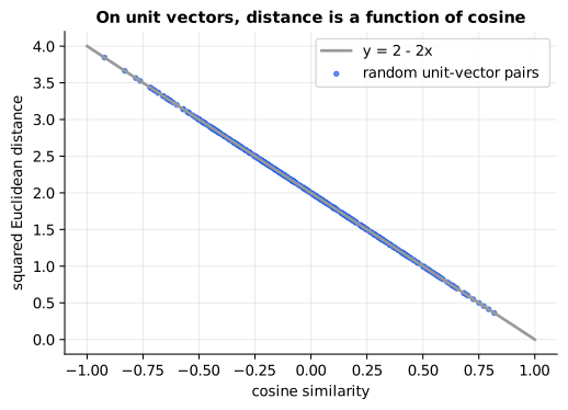
Reading it: each dot is one pair of random unit vectors. The horizontal axis is their cosine and the vertical axis is their squared Euclidean distance. Every dot sits exactly on the line y = 2 − 2x. Because the line only goes down, "higher cosine" and "smaller distance" always mean the same thing, so the two metrics can never disagree about which neighbour is nearer.
flowchart TD
  S{What was the model<br/>trained with?} -->|cosine| N[L2-normalize every vector<br/>once, at write time]
  S -->|dot product| D{Does the vector length<br/>carry signal?}
  D -->|yes, e.g. popularity| RAW[Keep raw vectors,<br/>rank by dot product]
  D -->|no| N
  N --> FAST[Rank by dot product:<br/>same order as cosine and L2,<br/>and the cheapest to compute]
Reading it: start at the top with the question that matters, which is how the model was trained, not which metric sounds best. Most text embedding models are trained with cosine, so you normalize once when you write vectors, then use the plain dot product at query time. It gives the same order as cosine and costs less. Only when length is deliberate signal do you skip normalizing.
In code: l2_normalize trims every row to length 1;
rankings_agree_after_normalizing ranks random documents by all three metrics
before and after normalizing and reports which rankings match, and
l2_identity_check returns both sides of the identity for two random vectors.
Why it matters: vector databases typically normalize on insert and then use the dot product, the cheapest of the three. If you mix normalized and unnormalized vectors, rankings quietly change. Use the metric the embedding model was trained with.
When length carries signal
Everyday picture: on the map of meaning, some shops are big and popular. A recommender may deliberately make popular items' arrows longer, so they win ties. Cosine throws that away; the dot product keeps it.
Tiny example (popularity_in_the_norm): the query points along
(1, 0). A niche item (0.99, 0.10) is almost perfectly aligned. A popular item
(0.95, 0.30) × 3 = (2.85, 0.90) is slightly off but three times longer.
| Item | Cosine with query | Dot with query |
|---|---|---|
| niche (0.99, 0.10) | 0.99 / 0.995 = 0.995 | 0.99 |
| popular (2.85, 0.90) | 2.85 / 2.99 = 0.954 | 2.85 |
Cosine prefers the niche item; the dot product prefers the popular one.
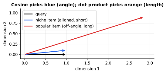
Reading it: the black arrow is the query. The blue arrow (niche item) points almost exactly the same way but is short. The orange arrow (popular item) leans a little away but is three times longer. Cosine only looks at the angle between each arrow and the query, so blue wins. The dot product also rewards length, so orange wins. Neither is wrong: it depends on what the model was trained to encode.
Why it matters: some retrieval and recommender models are trained with the raw dot product and put useful signal in the length. Normalizing their vectors "to be safe" throws that signal away.
The curse of dimensionality
Everyday picture: in a small village some neighbours live next door and some live across the valley. Now imagine a city with thousands of streets running in thousands of directions: pick random strangers and they all turn out to live about equally far from you. "Nearest" stops meaning much.
Tiny example: scatter 1,000 random points in a cube and measure from a random spot. In 2 dimensions the nearest point is about 1/100th as far away as the farthest. In 1,000 dimensions it's about 90% as far: everyone is nearly equidistant.
Level 3: the formula and its symbols
$$ \text{ratio} = \frac{\min_j \lVert q - x_j \rVert}{\max_j \lVert q - x_j \rVert} $$
Symbols
| Symbol | Meaning here | Shape / range |
|---|---|---|
| q | the query point | d numbers |
| xⱼ | the j-th of the random points | d numbers each |
| j | which random point | 1 to 1,000 |
| min, max over j | the smallest / largest value across all the points | |
| ratio | nearest distance divided by farthest distance | 0 to 1; near 1 means "all equally far" |
In words: the ratio is the distance to the closest point divided by the distance to the farthest point.
On the example: by hand first: a query at (0, 0) and three points at (1, 0), (0, 2) and (3, 4) are 1, 2 and 5 away, so the ratio is 1 / 5 = 0.2. With 1,000 random points the demo table shows about 0.01 at d = 2 and about 0.9 at d = 1,000. The Python below draws its own random points, so it lands close by rather than on the same digits: 0.02 and 0.9.
Level 3: in Python
In Python:
import math, random
def ratio(q, xs):
    # ‖q - x_j‖ for every j
    dists = [math.dist(q, x_j) for x_j in xs]
    # min over j ÷ max over j
    return min(dists) / max(dists)
ratio((0, 0), [(1, 0), (0, 2), (3, 4)])  # → 0.2
random.seed(0)
for d in (2, 1000):
    q = [random.random() for _ in range(d)]
    xs = [[random.random() for _ in range(d)] for _ in range(1000)]
    # one significant figure
    print(d, f"{ratio(q, xs):.1g}")  # → 2 0.02 1000 0.9
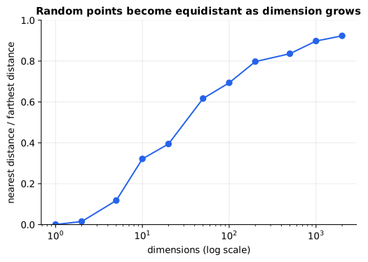
Reading it: the horizontal axis is the number of dimensions (log scale); the vertical axis is the nearest-to-farthest ratio above. In 2-D the ratio is near 0: the nearest point really is much nearer. By a few hundred dimensions the curve flattens toward 1, so every random point is roughly equally far away, and "nearest" tells you almost nothing about random data.
In code: curse_of_dimensionality scatters the random points, measures
from a random query, and returns the nearest, farthest and ratio for each
dimension.
Why it matters: exact nearest-neighbour search in high dimensions gets
slow and fragile, which is one reason vector search uses approximate indexes
(primer.ml.embeddings.ann). Real embeddings aren't random: meaning puts
them on a much lower-dimensional structure, so nearest-neighbour search still
works well in practice.
Anisotropy: why every score looks like 0.8
Everyday picture: a stadium crowd all facing the stage. Ask "are these two people facing the same way?" and the answer is "roughly yes" for everyone, so the question tells you little. Many embedding models behave like that crowd: their vectors bunch in a narrow cone, so even unrelated texts get cosines of 0.7 or more. This lopsidedness is called anisotropy ("not the same in every direction").
Tiny example: build each vector as √3·m + n, where m is one direction everybody shares (the stage) and n is a unit-length direction of each text's own. For two unrelated texts the n parts are at right angles, so their dot product is (√3)² = 3 and each length is √(3 + 1) = 2, and the cosine is 3 / (2 · 2) = 0.75. For paraphrases, whose own parts agree with cosine ρ, the cosine becomes 0.75 + 0.25·ρ: about 0.79 to 0.86. All the signal is squeezed into a few hundredths.
Level 3: the formula and its symbols
$$ v = \alpha\, m + \beta\, n, \qquad \cos(v_1, v_2) = \frac{\alpha^2 + \beta^2 \rho}{\alpha^2 + \beta^2} $$
Symbols
| Symbol | Meaning here | Shape / range |
|---|---|---|
| v, v₁, v₂ | an embedding vector | d numbers (768 here) |
| m | the shared direction every vector leans toward | unit vector |
| n | the text's own direction | unit vector |
| α (alpha) | how strongly every vector leans toward m | √3 here |
| β (beta) | how strongly each keeps its own direction | 1 here |
| ρ (rho) | cosine between the two texts' own directions | 0 unrelated; 0.15 to 0.45 for paraphrases |
In words: every vector is a big shared part plus a small personal part, so the cosine is mostly the shared part's weight, nudged up a little by how much the personal parts agree.
On the example: unrelated, ρ = 0: (3 + 0) / (3 + 1) = 0.75. A paraphrase with ρ = 0.4: (3 + 0.4) / 4 = 0.85.
Level 3: in Python
In Python:
import math
alpha, beta = math.sqrt(3), 1
# shared direction; two unrelated own directions
m, n1, n2 = (1, 0, 0), (0, 1, 0), (0, 0, 1)
# v = α m + β n
v1 = [alpha * m_i + beta * n_i for m_i, n_i in zip(m, n1)]
v2 = [alpha * m_i + beta * n_i for m_i, n_i in zip(m, n2)]
dot = sum(a * b for a, b in zip(v1, v2))
# the cosine, measured directly
round(dot / (math.hypot(*v1) * math.hypot(*v2)), 2)  # → 0.75
def cos_formula(rho):
    return (alpha ** 2 + beta ** 2 * rho) / (alpha ** 2 + beta ** 2)
# unrelated, and a paraphrase
round(cos_formula(0), 2), round(cos_formula(0.4), 2)  # → (0.75, 0.85)
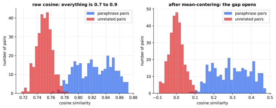
Reading it: the left panel shows raw cosine scores for 300 paraphrase pairs (one colour) and 300 unrelated pairs (the other). Both piles sit between 0.7 and 0.9, so a score of "0.8" alone says little. The right panel shows the same pairs after mean-centering, which means subtracting the average vector of the whole collection (that removes the shared "stage" direction). Unrelated pairs drop to about 0, paraphrases sit clearly above, and the gap is easy to see. The information was there all along, squeezed into a narrow band.
In code: anisotropic_embeddings builds the pairs as α·m + β·n,
pair_cosines scores each pair, and mean_center subtracts the average
vector to remove the shared direction.
Picking a threshold from data, not folklore
Sometimes you need a yes/no cut-off: "are these duplicates?", "is this cached answer close enough?". Pick it by measuring. Label some pairs, score them, and choose the threshold with the best F1, the balance of precision (of the pairs I called similar, how many were?) and recall (of the truly similar pairs, how many did I catch?):
Level 3: the formula and its symbols
$$ F_1 = \frac{2PR}{P + R} $$
Symbols
| Symbol | Meaning here | Range |
|---|---|---|
| P | precision: true matches ÷ everything called a match | 0 to 1 |
| R | recall: true matches found ÷ all true matches | 0 to 1 |
| F₁ | their harmonic mean; high only when both are high | 0 to 1 |
In words: F1 is twice the product of precision and recall, divided by their sum.
On a hand example: scores 0.9, 0.8, 0.7, 0.6 where the first two are true
matches. Threshold 0.8 calls exactly those two matches: P = 2/2 = 1,
R = 2/2 = 1, F₁ = 2·1·1 / 2 = 1. best_threshold finds 0.8.
Level 3: in Python
In Python:
scores = [0.9, 0.8, 0.7, 0.6]
# the labels
is_match = [True, True, False, False]
# threshold 0.8
called = [s >= 0.8 for s in scores]
true_matches = sum(c and y for c, y in zip(called, is_match))
# precision
P = true_matches / sum(called)
# recall
R = true_matches / sum(is_match)
# F₁
2 * P * R / (P + R)  # → 1.0
flowchart LR
  L[Sample a few hundred pairs<br/>from your own data] --> H[Label each:<br/>same meaning or not]
  H --> E[Score every pair<br/>with THIS model]
  E --> W[Sweep thresholds,<br/>compute precision, recall, F1]
  W --> P[Pick the threshold that fits<br/>your cost of each error]
  P --> V[Store it with the<br/>model version]
  V -->|model upgraded| E
Reading it: a threshold is a property of one model on one kind of data, so it is measured, not guessed. Label pairs, score them, sweep, and pick. The loop back from "model upgraded" is the step people forget: a new model has a different score distribution, so the old threshold is meaningless.
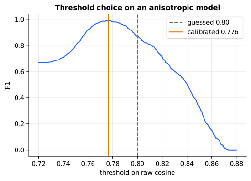
Reading it: the curve is F1 at each candidate threshold on the raw anisotropic scores. The dashed line is the "obvious" guess of 0.8; the solid line is the calibrated threshold. F1 changes sharply over a few hundredths of cosine, which is exactly why a threshold carried over from a different model (or a blog post) can be badly wrong.
In code: f1_curve computes F1 at every candidate threshold for this
plot; best_threshold returns the single best one with its precision and
recall.
Why it matters:
- Absolute scores mean different things for different models. "0.8" is not a universal "similar".
- Rank, don't threshold, whenever you can. A shared offset doesn't change which document is on top.
- When you must threshold (dedup, semantic caching, "no good answer found"), calibrate on labeled pairs for that model, and redo it when the model changes.
In 20 seconds
- Cosine compares direction, the dot product compares direction and length, Euclidean distance measures the gap between the tips.
- On L2-normalized vectors all three give the same ranking, because ‖a − b‖² = 2 − 2cos.
- Use the metric the model was trained with.
- Scores aren't comparable across models (anisotropy). Rank when you can; calibrate thresholds on labeled pairs when you can't.
Self-test questions
Q: When do cosine, dot product and Euclidean distance give the same ranking? When all vectors are L2-normalized: the dot product equals the cosine, and the squared distance equals 2 − 2cos, which always moves opposite to cosine.
Q: When would you deliberately use the raw dot product on unnormalized vectors? When the model was trained that way and encodes useful signal in the length (e.g. popularity or quality in some recommender and retrieval models). Normalizing would throw that signal away.
Q: Similarity scores all sit between 0.75 and 0.85. What's going on and how do you set a threshold? The model is anisotropic: its vectors share a dominant direction, so every pair looks similar and the real signal lives in a narrow band. Ranking still works. For a threshold, label a few hundred pairs from your own data, sweep the threshold, and pick the one that maximizes F1 (or matches your precision/recall needs). Optionally mean-center the vectors. Redo it for every model version.
Q: What is the curse of dimensionality for nearest-neighbour search? For random high-dimensional data, the nearest and farthest points are almost the same distance away, so "nearest" carries little information and exact search gets expensive. Real embeddings have structure, and approximate indexes trade a little recall for large speedups.
The papers behind this lesson
- Beyer, Goldstein, Ramakrishnan and Shaft, When Is "Nearest Neighbor" Meaningful? (1999): https://doi.org/10.1007/3-540-49257-7_15. Proved that for broad families of random data, the nearest and farthest neighbours become equally far as dimension grows: the curse of dimensionality measured in this lesson.
- Ethayarajh, How Contextual are Contextualized Word Representations? (2019): https://arxiv.org/abs/1909.00512. Showed that transformer embeddings occupy a narrow cone (anisotropy), which is why raw cosine scores bunch together.
- Su, Cao, Liu and Ou, Whitening Sentence Representations for Better Semantics and Faster Retrieval (2021): https://arxiv.org/abs/2103.15316. Showed that centering and whitening sentence embeddings spreads them back out and improves similarity quality.
Further reading
- Cosine similarity (Wikipedia): https://en.wikipedia.org/wiki/Cosine_similarity
- Beyer et al., When Is "Nearest Neighbor" Meaningful? (1999): https://doi.org/10.1007/3-540-49257-7_15
- Ethayarajh, How Contextual are Contextualized Word Representations? (anisotropy, 2019): https://arxiv.org/abs/1909.00512
- Su et al., Whitening Sentence Representations (2021): https://arxiv.org/abs/2103.15316
- sentence-transformers, semantic search and score functions: https://www.sbert.net/examples/applications/semantic-search/README.html
1r""" 2# Similarity: how close are two meanings? 3 4Run: `python -m primer.ml.embeddings.similarity` 5 6New to the notation (vectors, Σ, ‖x‖)? Start with `primer.notation`, which 7builds every symbol used here from zero. 8 9## Level 1: The practitioner's guide 10 11**In one sentence.** A similarity metric turns two embedding vectors into 12one number that says how alike their meanings are, and the three in common 13use (cosine, dot product, Euclidean distance) agree with each other only 14under conditions you have to arrange. 15 16**When you need it.** Every time you compare embeddings: semantic search, 17retrieval for RAG, near-duplicate detection, a semantic cache that answers a 18question from a stored one, clustering, recommendations. You choose a metric 19whether you mean to or not, because every vector database and every search 20library has a default, and the wrong one ranks silently wrong. The tells: 21you are about to write `ORDER BY` against a vector column and have not 22checked which operator the embedding model expects; or your team argues 23about whether "0.8 similar" is a lot. This lesson's demo shows why the 24second argument can't be settled by intuition: for one model, paraphrases 25score between 0.76 and 0.87 and unrelated pairs between 0.72 and 0.78, so 26"0.8" is either a near-duplicate or a stranger. You don't need any of this 27for exact-match lookups (an id, a hash) or for keyword search, which scores 28words, not vectors. 29 30**Your options.** The ways to score a pair, from the cheapest to the most 31deliberate: 32 33| Option | What it does | What it guarantees | What it costs | Where it lives | 34|---|---|---|---|---| 35| Dot product on normalized vectors | Normalize every vector to length 1 once, at write time, then multiply and add | The same ranking as cosine and as Euclidean distance, at the lowest price | One multiply-add per dimension per pair; a normalization step on insert | Your ingestion code, then the database's inner-product operator | 36| Cosine similarity | Dot product divided by both lengths | Direction only; lengths can't skew the order, whatever came in | Two extra norms per comparison, unless the store caches them | The database's cosine operator, or a library's default | 37| Raw dot product | Direction and length together | Keeps signal a model put in the length, such as popularity | Rankings that a mix of long and short vectors can dominate | Recommenders and models trained with it | 38| Euclidean distance | Straight-line gap between the tips | The natural metric for clustering and for many index structures | Disagrees with cosine unless vectors are normalized | k-means, some indexes | 39| Mean-centred scores | Subtract the collection's average vector before comparing | Unrelated pairs land near 0, similar ones stand clear | A pass over the collection, and a re-run when it changes | Your code, before scoring | 40| A calibrated threshold | Label a few hundred pairs, sweep the cut-off, keep the best F1 | A yes/no that matches your data and your model | A labelling session, repeated at every model change | A number stored with the model version | 41 42**How to choose.** Start from how the model was trained, not from which 43metric sounds best. 44 45- The model's documentation says cosine, or says its vectors are unit 46 length (most text embedding APIs): normalize on write and rank by dot 47 product. Same order as cosine, fewer operations. 48- The model was trained with a raw dot product and encodes something in the 49 length (recommenders, some retrieval models): keep raw vectors and use the 50 dot product. Normalizing "to be safe" throws the signal away. 51- You need an ordered list (search, RAG): rank, and never threshold. A shared 52 offset in every score leaves the order alone. 53- You need a yes/no (duplicates, a cache hit, "no good answer found"): 54 calibrate the threshold on labelled pairs from your own data, for this 55 model, and store it with the model version. 56- Whatever you pick, use one metric, one model and one normalization policy 57 for every vector in the index. A mixture ranks wrong without an error. 58 59**What it costs.** A comparison is arithmetic over the vector's dimensions: 60real models produce 384 to 3,072 numbers per text, so a dot product is a few 61thousand multiply-adds, and cosine adds two square roots and a division 62unless the lengths are precomputed. Exact search is one comparison per 63stored vector; the sentence-transformers documentation puts the practical 64limit of that brute-force loop at about a million entries, after which you 65move to an approximate index (`primer.ml.embeddings.ann`). Storage is 4 bytes 66per dimension as float32 (pgvector charges 4 × dimensions + 8 bytes per 67vector, half that as 16-bit floats), which `primer.ml.embeddings.compression` 68shrinks. Normalizing is one pass at write time, once. Calibration costs 69labelling: a few hundred pairs, scored and swept, and the demo shows the 70return on it: a guessed threshold of 0.80 reaches F1 0.868 on the demo's 71pairs, the calibrated 0.776 reaches 0.992. 72 73**What breaks.** 74 75- **Mixed normalization.** Some vectors normalized, some not, and the 76 ranking quietly changes: in the demo, raw dot product and cosine order 200 77 documents differently, and agree only after every vector is normalized. 78 Normalize in one place, on the write path. 79- **A threshold from folklore.** A cut-off copied from a blog post or from 80 the previous model is meaningless: F1 swings from 0.99 to 0.87 across four 81 hundredths of cosine. Measure it on labelled pairs, per model. 82- **Every score looks like 0.8.** Transformer embeddings crowd into a narrow 83 cone (Ethayarajh, 2019, found them "not isotropic in any layer"). Rank 84 instead of judging absolute scores, or mean-centre: after centring, the 85 demo's unrelated pairs sit at 0.00 and paraphrases at 0.30. 86- **A model upgrade with an old index.** A new model is a new space: old 87 vectors, old thresholds and old scores don't carry over. Re-embed the whole 88 collection and recalibrate (`primer.ml.embeddings.operations`). 89- **The operator is a distance, not a similarity.** Databases often expose 90 cosine *distance* (1 − cosine) and the *negative* inner product so that 91 ascending order is best-first, as pgvector does. Read the sign before you 92 sort. 93- **Queries and documents embedded differently.** Some providers train 94 separate treatments for the query and for the passage (Cohere's 95 `input_type` of search_query and search_document); embed both sides the way 96 the model expects or the scores are off. 97- **Nearest means little on unstructured data.** With 1,000 random points, 98 the nearest is 0.7% as far as the farthest in 2 dimensions and 90% as far 99 in 1,000: the curse of dimensionality. Real embeddings are structured, so 100 search works, but a score gap that small is a warning that the vectors 101 carry little. 102 103**In the wild.** pgvector exposes one operator per metric on a Postgres 104column: `<->` for Euclidean distance, `<#>` for the negative inner product, 105`<=>` for cosine distance, plus Hamming and Jaccard on bit vectors, up to 10616,000 dimensions. sentence-transformers' semantic search defaults to cosine 107and offers dot-product scoring for normalized vectors. OpenAI's embedding 108guide states that its embeddings are normalized to length 1, recommends 109cosine, and notes that it can then be computed as a plain dot product; Cohere 110asks for an `input_type` per side of the search. Faiss's flat indexes 111(IndexFlatIP, IndexFlatL2) are the exact inner-product and Euclidean 112searches every approximate index is measured against. Ethayarajh (2019) 113measured anisotropy in contextual models and Su et al. (2021) showed that 114centring and whitening spreads the vectors back out. 115 116**Go deeper.** Level 2 computes all three metrics by hand on three 1173-dimensional vectors, proves in one line why normalizing makes them agree 118(the squared distance is 2 − 2 × cosine), builds the popularity example where 119cosine and dot product disagree on purpose, measures the curse of 120dimensionality with random points, and manufactures anisotropic embeddings 121to show a calibrated threshold beating a guessed one. If you only needed to 122choose, you are done. 123 124## Level 2: How it works, from scratch 125 126An **embedding** gives every piece of text a set of coordinates on a map of 127meaning. Texts about similar things live on the same street; unrelated ones 128are across town. Draw an arrow from the centre of the map to each text's 129spot, and "how similar are these two texts?" becomes "how alike are these two 130arrows?". 131 132There are three natural ways to compare two arrows: 133 134- **Cosine similarity** compares the *direction* they point and ignores how 135 long they are, like two people pointing at the same mountain, one with a 136 longer arm. 137- **Euclidean distance** is the straight-line distance between the two arrow 138 tips, like measuring with a ruler. 139- **Dot product** mixes both: pointing the same way *and* being long both 140 make it bigger. 141 142## A tiny worked example 143 144Three texts, each placed in a 3-dimensional space (real models use 384 to 1453,072 **dimensions**, meaning numbers per vector; the arithmetic is the same): 146 147a = (1, 2, 2), b = (2, 1, 2), c = (2, −1, −2) 148 1491. **Dot product**: multiply position by position, then add. 150 a·b = 1·2 + 2·1 + 2·2 = **8**. a·c = 1·2 + 2·(−1) + 2·(−2) = **−4**. 1512. **Length** (the **norm**, written ‖a‖): square each number, add, and take 152 the square root. ‖a‖ = √(1 + 4 + 4) = **3**, and b and c also have length 3. 1533. **Cosine**: dot product divided by both lengths. 154 cos(a, b) = 8 / (3·3) = **0.89**. cos(a, c) = −4 / 9 = **−0.44**. 1554. **Euclidean distance**: subtract, square, add, square-root. 156 ‖a − b‖ = √(1 + 1 + 0) = **1.41**. ‖a − c‖ = √(1 + 9 + 16) = **5.10**. 157 158| Pair | Dot product | Lengths multiplied | Cosine | Distance | Reading | 159|---|---|---|---|---|---| 160| a, b | 8 | 9 | 0.89 | 1.41 | Very similar | 161| a, c | −4 | 9 | −0.44 | 5.10 | Pointing away | 162 163Cosine runs from −1 (opposite directions) through 0 (unrelated, at right 164angles) to 1 (same direction). 165 166```mermaid 167flowchart LR 168 A["a = (1, 2, 2)"] --> D["dot product<br/>a·b = 8"] 169 B["b = (2, 1, 2)"] --> D 170 A --> NA["length ‖a‖ = 3"] 171 B --> NB["length ‖b‖ = 3"] 172 D --> COS["cosine = 8 / (3 × 3) = 0.89"] 173 NA --> COS 174 NB --> COS 175 A --> SUB["difference a − b = (−1, 1, 0)"] 176 B --> SUB 177 SUB --> L2["distance = √2 = 1.41"] 178``` 179 180**Reading it:** the two input vectors feed three calculations. The top path 181is the dot product. The middle paths measure each vector's length, and 182cosine is simply the dot product divided by those lengths, which is how it 183comes to "ignore length". The bottom path subtracts the vectors and measures 184what's left: that's distance. Everything later in this lesson is these three 185boxes. 186 187**In code:** `worked_example` computes every number in the table above from 188a, b and c, so you can check your hand arithmetic against it. 189 190## The math 191 192$$ 193\cos(a, b) = \frac{a \cdot b}{\lVert a \rVert \, \lVert b \rVert} 194\qquad 195a \cdot b = \sum_{i=1}^{d} a_i b_i 196\qquad 197\lVert a - b \rVert = \sqrt{\sum_{i=1}^{d} (a_i - b_i)^2} 198$$ 199 200**Symbols** 201 202| Symbol | Meaning here | Shape / range | 203|---|---|---| 204| a, b | the two embedding vectors being compared | d numbers each | 205| d | number of dimensions | 3 in the example; 384 to 3,072 in real models | 206| i | which position (dimension) we're looking at | 1 to d | 207| aᵢ | the i-th number in a | a real number | 208| Σ | "add up", over i from 1 to d | | 209| a · b | dot product: multiply matching positions and add | one number, any sign | 210| ‖a‖ | length (norm) of a: √(Σ aᵢ²) | one number ≥ 0 | 211| √ | square root | | 212| cos(a, b) | cosine of the angle between a and b | −1 to 1 | 213| ‖a − b‖ | Euclidean distance between the tips | ≥ 0; 0 means identical | 214 215**In words:** the cosine of a and b is their dot product divided by the 216product of their lengths; the dot product adds up the products of matching 217positions; the distance is the square root of the summed squared 218differences. 219 220**On the example:** cos(a, b) = (1·2 + 2·1 + 2·2) / (3 · 3) = 8 / 9 = 0.89; 221‖a − b‖ = √((1−2)² + (2−1)² + (2−2)²) = √2 = 1.41. 222 223**In Python:** 224 225```python 226import math 227a, b = [1, 2, 2], [2, 1, 2] 228# a · b = Σ a_i b_i 229dot = sum(a_i * b_i for a_i, b_i in zip(a, b)) 230dot # → 8 231# ‖a‖ 232norm_a = math.sqrt(sum(a_i ** 2 for a_i in a)) 233# ‖b‖ 234norm_b = math.sqrt(sum(b_i ** 2 for b_i in b)) 235norm_a, norm_b # → (3.0, 3.0) 236# cos(a, b) 237round(dot / (norm_a * norm_b), 2) # → 0.89 238# ‖a - b‖ 239round(math.sqrt(sum((a_i - b_i) ** 2 for a_i, b_i in zip(a, b))), 2) # → 1.41 240``` 241 242The code is `cosine`, `dot` and `euclidean`, each a line of NumPy. 243 244**In code:** `rank` sorts a whole collection of documents from best to worst 245match under whichever of the three metrics you name. 246 247**Why it matters:** every vector database, semantic search box and RAG 248system does exactly this comparison, millions of times per second. Knowing 249which of the three a system uses, and why, is the difference between 250correct and silently wrong rankings. 251 252## Normalize, and the three agree 253 254**Everyday picture:** trim every arrow to the same length, one unit. Now the 255only thing that can differ is direction, so "tips are close together" and 256"arrows point the same way" become the same statement. 257 258**Tiny example:** a = (1, 0) and b = (0.6, 0.8) both have length 1 (check: 2590.6² + 0.8² = 0.36 + 0.64 = 1). Their cosine is 1·0.6 + 0·0.8 = 0.6. The squared 260distance is (1 − 0.6)² + (0 − 0.8)² = 0.16 + 0.64 = 0.8, and 2 − 2·0.6 = 0.8. 261Same number. 262 263$$ 264\lVert a - b \rVert^2 = \lVert a \rVert^2 + \lVert b \rVert^2 - 2\,a\cdot b = 2 - 2\cos(a, b) 265\quad \text{when } \lVert a \rVert = \lVert b \rVert = 1 266$$ 267 268**Symbols** 269 270| Symbol | Meaning here | Shape / range | 271|---|---|---| 272| ‖a − b‖² | squared distance between the tips | 0 to 4 for unit vectors | 273| ‖a‖², ‖b‖² | squared lengths, both 1 after normalizing | 1 | 274| a · b | dot product, equal to cosine for unit vectors | −1 to 1 | 275| cos(a, b) | cosine similarity | −1 to 1 | 276 277**In words:** for unit-length vectors, the squared distance is two minus 278twice the cosine, so the higher the cosine, the smaller the distance, always. 279 280**On the example:** ‖a − b‖² = 1 + 1 − 2·0.6 = 0.8 = 2 − 2·0.6. 281 282**In Python:** 283 284```python 285# both length 1 286a, b = [1, 0], [0.6, 0.8] 287# for unit vectors, a · b is the cosine 288cos = sum(a_i * b_i for a_i, b_i in zip(a, b)) 289# ‖a - b‖² 290dist_sq = sum((a_i - b_i) ** 2 for a_i, b_i in zip(a, b)) 291# the two sides of the identity 292round(dist_sq, 2), round(2 - 2 * cos, 2) # → (0.8, 0.8) 293``` 294 295**L2-normalizing** (dividing a vector by its own length) is what trims every 296arrow to length 1. After it, the dot product *is* the cosine, and distance is 297a decreasing function of the cosine. So **once vectors are L2-normalized, 298cosine, dot product and Euclidean distance give the same ranking.** 299 300**Try it:** pick "Same direction, different lengths", then drag B's length. 301The dot product and the distance change, but the cosine stays at 1, because 302it only sees the angle. Drag an angle instead and watch the cosine slide from 3031 through 0 to −1. Then switch on "Normalize to length 1": both arrows shrink 304to the unit circle, the dot product becomes the cosine, and the squared 305distance becomes 2 − 2 × cosine. 306 307<div class="viz" data-viz="cosine-similarity" aria-label="Cosine similarity of two arrows"></div> 308 309 310 311**Reading it:** each dot is one pair of random unit vectors. The horizontal 312axis is their cosine and the vertical axis is their squared Euclidean 313distance. Every dot sits exactly on the line y = 2 − 2x. Because the line only 314goes down, "higher cosine" and "smaller distance" always mean the same thing, 315so the two metrics can never disagree about which neighbour is nearer. 316 317```mermaid 318flowchart TD 319 S{What was the model<br/>trained with?} -->|cosine| N[L2-normalize every vector<br/>once, at write time] 320 S -->|dot product| D{Does the vector length<br/>carry signal?} 321 D -->|yes, e.g. popularity| RAW[Keep raw vectors,<br/>rank by dot product] 322 D -->|no| N 323 N --> FAST[Rank by dot product:<br/>same order as cosine and L2,<br/>and the cheapest to compute] 324``` 325 326**Reading it:** start at the top with the question that matters, which is 327how the model was trained, not which metric sounds best. Most text 328embedding models are trained with cosine, so you normalize once when you 329write vectors, then use the plain dot product at query time. It gives the 330same order as cosine and costs less. Only when length is deliberate signal 331do you skip normalizing. 332 333**In code:** `l2_normalize` trims every row to length 1; 334`rankings_agree_after_normalizing` ranks random documents by all three metrics 335before and after normalizing and reports which rankings match, and 336`l2_identity_check` returns both sides of the identity for two random vectors. 337 338**Why it matters:** vector databases typically normalize on insert and 339then use the dot product, the cheapest of the three. If you mix normalized 340and unnormalized vectors, rankings quietly change. **Use the metric the 341embedding model was trained with.** 342 343## When length carries signal 344 345**Everyday picture:** on the map of meaning, some shops are big and popular. 346A recommender may deliberately make popular items' arrows longer, so they 347win ties. Cosine throws that away; the dot product keeps it. 348 349**Tiny example** (`popularity_in_the_norm`): the query points along 350(1, 0). A niche item (0.99, 0.10) is almost perfectly aligned. A popular item 351(0.95, 0.30) × 3 = (2.85, 0.90) is slightly off but three times longer. 352 353| Item | Cosine with query | Dot with query | 354|---|---|---| 355| niche (0.99, 0.10) | 0.99 / 0.995 = 0.995 | 0.99 | 356| popular (2.85, 0.90) | 2.85 / 2.99 = 0.954 | 2.85 | 357 358Cosine prefers the niche item; the dot product prefers the popular one. 359 360 361 362**Reading it:** the black arrow is the query. The blue arrow (niche item) 363points almost exactly the same way but is short. The orange arrow (popular 364item) leans a little away but is three times longer. Cosine only looks at 365the angle between each arrow and the query, so blue wins. The dot product 366also rewards length, so orange wins. Neither is wrong: it depends on what 367the model was trained to encode. 368 369**Why it matters:** some retrieval and recommender models are trained with 370the raw dot product and put useful signal in the length. Normalizing their 371vectors "to be safe" throws that signal away. 372 373## The curse of dimensionality 374 375**Everyday picture:** in a small village some neighbours live next door and 376some live across the valley. Now imagine a city with thousands of streets 377running in thousands of directions: pick random strangers and they all turn 378out to live about equally far from you. "Nearest" stops meaning much. 379 380**Tiny example:** scatter 1,000 random points in a cube and measure from a 381random spot. In 2 dimensions the nearest point is about 1/100th as far away 382as the farthest. In 1,000 dimensions it's about 90% as far: everyone is 383nearly equidistant. 384 385$$ 386\text{ratio} = \frac{\min_j \lVert q - x_j \rVert}{\max_j \lVert q - x_j \rVert} 387$$ 388 389**Symbols** 390 391| Symbol | Meaning here | Shape / range | 392|---|---|---| 393| q | the query point | d numbers | 394| xⱼ | the j-th of the random points | d numbers each | 395| j | which random point | 1 to 1,000 | 396| min, max over j | the smallest / largest value across all the points | | 397| ratio | nearest distance divided by farthest distance | 0 to 1; near 1 means "all equally far" | 398 399**In words:** the ratio is the distance to the closest point divided by the 400distance to the farthest point. 401 402**On the example:** by hand first: a query at (0, 0) and three points at 403(1, 0), (0, 2) and (3, 4) are 1, 2 and 5 away, so the ratio is 1 / 5 = 0.2. 404With 1,000 random points the demo table shows about 0.01 at d = 2 and about 4050.9 at d = 1,000. The Python below draws its own random points, so it lands 406close by rather than on the same digits: 0.02 and 0.9. 407 408**In Python:** 409 410```python 411import math, random 412def ratio(q, xs): 413 # ‖q - x_j‖ for every j 414 dists = [math.dist(q, x_j) for x_j in xs] 415 # min over j ÷ max over j 416 return min(dists) / max(dists) 417ratio((0, 0), [(1, 0), (0, 2), (3, 4)]) # → 0.2 418random.seed(0) 419for d in (2, 1000): 420 q = [random.random() for _ in range(d)] 421 xs = [[random.random() for _ in range(d)] for _ in range(1000)] 422 # one significant figure 423 print(d, f"{ratio(q, xs):.1g}") # → 2 0.02 1000 0.9 424``` 425 426 427 428**Reading it:** the horizontal axis is the number of dimensions (log scale); 429the vertical axis is the nearest-to-farthest ratio above. In 2-D the ratio is 430near 0: the nearest point really is much nearer. By a few hundred dimensions 431the curve flattens toward 1, so every random point is roughly equally far 432away, and "nearest" tells you almost nothing about random data. 433 434**In code:** `curse_of_dimensionality` scatters the random points, measures 435from a random query, and returns the nearest, farthest and ratio for each 436dimension. 437 438**Why it matters:** exact nearest-neighbour search in high dimensions gets 439slow and fragile, which is one reason vector search uses approximate indexes 440(`primer.ml.embeddings.ann`). Real embeddings aren't random: meaning puts 441them on a much lower-dimensional structure, so nearest-neighbour search still 442works well in practice. 443 444## Anisotropy: why every score looks like 0.8 445 446**Everyday picture:** a stadium crowd all facing the stage. Ask "are these 447two people facing the same way?" and the answer is "roughly yes" for 448everyone, so the question tells you little. Many embedding models behave 449like that crowd: their vectors bunch in a narrow cone, so even unrelated 450texts get cosines of 0.7 or more. This lopsidedness is called 451**anisotropy** ("not the same in every direction"). 452 453**Tiny example:** build each vector as √3·m + n, where m is one direction 454everybody shares (the stage) and n is a unit-length direction of each 455text's own. For two unrelated texts the n parts are at right angles, so 456their dot product is (√3)² = 3 and each length is √(3 + 1) = 2, and the 457cosine is 3 / (2 · 2) = **0.75**. For paraphrases, whose own parts agree with 458cosine ρ, the cosine becomes 0.75 + 0.25·ρ: about 0.79 to 0.86. All the signal 459is squeezed into a few hundredths. 460 461$$ 462v = \alpha\, m + \beta\, n, \qquad 463\cos(v_1, v_2) = \frac{\alpha^2 + \beta^2 \rho}{\alpha^2 + \beta^2} 464$$ 465 466**Symbols** 467 468| Symbol | Meaning here | Shape / range | 469|---|---|---| 470| v, v₁, v₂ | an embedding vector | d numbers (768 here) | 471| m | the shared direction every vector leans toward | unit vector | 472| n | the text's own direction | unit vector | 473| α (alpha) | how strongly every vector leans toward m | √3 here | 474| β (beta) | how strongly each keeps its own direction | 1 here | 475| ρ (rho) | cosine between the two texts' own directions | 0 unrelated; 0.15 to 0.45 for paraphrases | 476 477**In words:** every vector is a big shared part plus a small personal part, 478so the cosine is mostly the shared part's weight, nudged up a little by how 479much the personal parts agree. 480 481**On the example:** unrelated, ρ = 0: (3 + 0) / (3 + 1) = 0.75. A paraphrase with 482ρ = 0.4: (3 + 0.4) / 4 = 0.85. 483 484**In Python:** 485 486```python 487import math 488alpha, beta = math.sqrt(3), 1 489# shared direction; two unrelated own directions 490m, n1, n2 = (1, 0, 0), (0, 1, 0), (0, 0, 1) 491# v = α m + β n 492v1 = [alpha * m_i + beta * n_i for m_i, n_i in zip(m, n1)] 493v2 = [alpha * m_i + beta * n_i for m_i, n_i in zip(m, n2)] 494dot = sum(a * b for a, b in zip(v1, v2)) 495# the cosine, measured directly 496round(dot / (math.hypot(*v1) * math.hypot(*v2)), 2) # → 0.75 497def cos_formula(rho): 498 return (alpha ** 2 + beta ** 2 * rho) / (alpha ** 2 + beta ** 2) 499# unrelated, and a paraphrase 500round(cos_formula(0), 2), round(cos_formula(0.4), 2) # → (0.75, 0.85) 501``` 502 503 504 505**Reading it:** the left panel shows raw cosine scores for 300 paraphrase 506pairs (one colour) and 300 unrelated pairs (the other). Both piles sit 507between 0.7 and 0.9, so a score of "0.8" alone says little. The right panel 508shows the same pairs after **mean-centering**, which means subtracting the 509average vector of the whole collection (that removes the shared "stage" 510direction). Unrelated pairs drop to about 0, paraphrases sit clearly above, 511and the gap is easy to see. The information was there all along, squeezed 512into a narrow band. 513 514**In code:** `anisotropic_embeddings` builds the pairs as α·m + β·n, 515`pair_cosines` scores each pair, and `mean_center` subtracts the average 516vector to remove the shared direction. 517 518### Picking a threshold from data, not folklore 519 520Sometimes you need a yes/no cut-off: "are these duplicates?", "is this 521cached answer close enough?". Pick it by measuring. Label some pairs, 522score them, and choose the threshold with the best **F1**, the balance of 523**precision** (of the pairs I called similar, how many were?) and **recall** 524(of the truly similar pairs, how many did I catch?): 525 526$$ 527F_1 = \frac{2PR}{P + R} 528$$ 529 530**Symbols** 531 532| Symbol | Meaning here | Range | 533|---|---|---| 534| P | precision: true matches ÷ everything called a match | 0 to 1 | 535| R | recall: true matches found ÷ all true matches | 0 to 1 | 536| F₁ | their harmonic mean; high only when both are high | 0 to 1 | 537 538**In words:** F1 is twice the product of precision and recall, divided by 539their sum. 540 541**On a hand example:** scores 0.9, 0.8, 0.7, 0.6 where the first two are true 542matches. Threshold 0.8 calls exactly those two matches: P = 2/2 = 1, 543R = 2/2 = 1, F₁ = 2·1·1 / 2 = 1. `best_threshold` finds 0.8. 544 545**In Python:** 546 547```python 548scores = [0.9, 0.8, 0.7, 0.6] 549# the labels 550is_match = [True, True, False, False] 551# threshold 0.8 552called = [s >= 0.8 for s in scores] 553true_matches = sum(c and y for c, y in zip(called, is_match)) 554# precision 555P = true_matches / sum(called) 556# recall 557R = true_matches / sum(is_match) 558# F₁ 5592 * P * R / (P + R) # → 1.0 560``` 561 562```mermaid 563flowchart LR 564 L[Sample a few hundred pairs<br/>from your own data] --> H[Label each:<br/>same meaning or not] 565 H --> E[Score every pair<br/>with THIS model] 566 E --> W[Sweep thresholds,<br/>compute precision, recall, F1] 567 W --> P[Pick the threshold that fits<br/>your cost of each error] 568 P --> V[Store it with the<br/>model version] 569 V -->|model upgraded| E 570``` 571 572**Reading it:** a threshold is a property of one model on one kind of data, 573so it is *measured*, not guessed. Label pairs, score them, sweep, and pick. 574The loop back from "model upgraded" is the step people forget: a new model 575has a different score distribution, so the old threshold is meaningless. 576 577 578 579**Reading it:** the curve is F1 at each candidate threshold on the raw 580anisotropic scores. The dashed line is the "obvious" guess of 0.8; the 581solid line is the calibrated threshold. F1 changes sharply over a few 582hundredths of cosine, which is exactly why a threshold carried over from a 583different model (or a blog post) can be badly wrong. 584 585**In code:** `f1_curve` computes F1 at every candidate threshold for this 586plot; `best_threshold` returns the single best one with its precision and 587recall. 588 589**Why it matters:** 590 591* Absolute scores mean different things for different models. "0.8" is 592 not a universal "similar". 593* **Rank, don't threshold, whenever you can.** A shared offset doesn't change 594 which document is on top. 595* When you *must* threshold (dedup, semantic caching, "no good answer 596 found"), calibrate on labeled pairs for that model, and redo it when the 597 model changes. 598 599## In 20 seconds 600- Cosine compares direction, the dot product compares direction and length, 601 Euclidean distance measures the gap between the tips. 602- On L2-normalized vectors all three give the same ranking, because 603 ‖a − b‖² = 2 − 2cos. 604- Use the metric the model was trained with. 605- Scores aren't comparable across models (anisotropy). Rank when you can; 606 calibrate thresholds on labeled pairs when you can't. 607 608## Self-test questions 609 610**Q: When do cosine, dot product and Euclidean distance give the same ranking?** 611When all vectors are L2-normalized: the dot product equals the cosine, and 612the squared distance equals 2 − 2cos, which always moves opposite to cosine. 613 614**Q: When would you deliberately use the raw dot product on unnormalized vectors?** 615When the model was trained that way and encodes useful signal in the length 616(e.g. popularity or quality in some recommender and retrieval models). 617Normalizing would throw that signal away. 618 619**Q: Similarity scores all sit between 0.75 and 0.85. What's going on and how do you set a threshold?** 620The model is anisotropic: its vectors share a dominant direction, so every 621pair looks similar and the real signal lives in a narrow band. Ranking still 622works. For a threshold, label a few hundred pairs from your own data, sweep 623the threshold, and pick the one that maximizes F1 (or matches your 624precision/recall needs). Optionally mean-center the vectors. Redo it for 625every model version. 626 627**Q: What is the curse of dimensionality for nearest-neighbour search?** 628For random high-dimensional data, the nearest and farthest points are almost 629the same distance away, so "nearest" carries little information and exact 630search gets expensive. Real embeddings have structure, and approximate 631indexes trade a little recall for large speedups. 632 633## The papers behind this lesson 634 635- **Beyer, Goldstein, Ramakrishnan and Shaft, *When Is "Nearest Neighbor" Meaningful?* (1999)**: https://doi.org/10.1007/3-540-49257-7_15. 636 Proved that for broad families of random data, the nearest and farthest neighbours become equally far as dimension grows: the curse of dimensionality measured in this lesson. 637- **Ethayarajh, *How Contextual are Contextualized Word Representations?* (2019)**: https://arxiv.org/abs/1909.00512. 638 Showed that transformer embeddings occupy a narrow cone (anisotropy), which is why raw cosine scores bunch together. 639- **Su, Cao, Liu and Ou, *Whitening Sentence Representations for Better Semantics and Faster Retrieval* (2021)**: https://arxiv.org/abs/2103.15316. 640 Showed that centering and whitening sentence embeddings spreads them back out and improves similarity quality. 641 642## Further reading 643- Cosine similarity (Wikipedia): https://en.wikipedia.org/wiki/Cosine_similarity 644- Beyer et al., *When Is "Nearest Neighbor" Meaningful?* (1999): https://doi.org/10.1007/3-540-49257-7_15 645- Ethayarajh, *How Contextual are Contextualized Word Representations?* (anisotropy, 2019): https://arxiv.org/abs/1909.00512 646- Su et al., *Whitening Sentence Representations* (2021): https://arxiv.org/abs/2103.15316 647- sentence-transformers, semantic search and score functions: https://www.sbert.net/examples/applications/semantic-search/README.html 648""" 649 650from __future__ import annotations 651 652import numpy as np 653 654from primer._show import banner, say, table, takeaway 655 656# --------------------------------------------------------------------------- 657# 1. The three measures 658# --------------------------------------------------------------------------- 659 660 661def l2_normalize(X: np.ndarray, axis: int = -1, eps: float = 1e-12) -> np.ndarray: 662 """Scale each vector (row, by default) to unit length. 663 664 `eps` avoids dividing by zero for an all-zero vector (e.g. empty text). 665 """ 666 return X / np.maximum(np.linalg.norm(X, axis=axis, keepdims=True), eps) 667 668 669def dot(a: np.ndarray, b: np.ndarray) -> float: 670 """Sum of element-wise products. Sensitive to both angle and length.""" 671 return float(np.dot(a, b)) 672 673 674def cosine(a: np.ndarray, b: np.ndarray) -> float: 675 """cos(angle) = a·b / (|a||b|). In [-1, 1]; ignores length.""" 676 return float(np.dot(a, b) / (np.linalg.norm(a) * np.linalg.norm(b))) 677 678 679def euclidean(a: np.ndarray, b: np.ndarray) -> float: 680 """Straight-line distance. Smaller means closer.""" 681 return float(np.linalg.norm(a - b)) 682 683 684def rank(query: np.ndarray, docs: np.ndarray, metric: str) -> np.ndarray: 685 """Doc indices from best to worst match under `metric` (cosine | dot | l2).""" 686 if metric == "dot": 687 scores = docs @ query 688 elif metric == "cosine": 689 scores = (docs @ query) / (np.linalg.norm(docs, axis=1) * np.linalg.norm(query)) 690 elif metric == "l2": 691 scores = -np.linalg.norm(docs - query, axis=1) # negate: closer = higher 692 else: 693 raise ValueError(metric) 694 # Stable sort so ties break the same way for every metric. 695 return np.argsort(-scores, kind="stable") 696 697 698# --------------------------------------------------------------------------- 699# 2. Worked example 700# --------------------------------------------------------------------------- 701 702A = np.array([1.0, 2.0, 2.0]) 703B = np.array([2.0, 1.0, 2.0]) 704C = np.array([2.0, -1.0, -2.0]) 705 706 707def worked_example() -> dict[str, float]: 708 """a, b, c from the table above. Returns the numbers you should be able to compute by hand.""" 709 return { 710 "len_a": float(np.linalg.norm(A)), 711 "dot_ab": dot(A, B), 712 "dot_ac": dot(A, C), 713 "cos_ab": cosine(A, B), 714 "cos_ac": cosine(A, C), 715 "l2_ab": euclidean(A, B), 716 "l2_ac": euclidean(A, C), 717 } 718 719 720# --------------------------------------------------------------------------- 721# 3. Normalization makes the metrics agree; without it they can disagree 722# --------------------------------------------------------------------------- 723 724 725def rankings_agree_after_normalizing(n_docs: int = 200, dim: int = 32, seed: int = 0) -> dict[str, bool]: 726 """Random docs with wildly different lengths: do the three rankings agree? 727 728 Before normalizing: dot product favors long vectors, so it disagrees. 729 After normalizing: all three rankings are identical, as the algebra says. 730 """ 731 rng = np.random.default_rng(seed) 732 docs = rng.standard_normal((n_docs, dim)) * rng.uniform(0.2, 5.0, (n_docs, 1)) # varied lengths 733 q = rng.standard_normal(dim) 734 735 raw = {m: rank(q, docs, m) for m in ("cosine", "dot", "l2")} 736 dn, qn = l2_normalize(docs), l2_normalize(q) 737 norm = {m: rank(qn, dn, m) for m in ("cosine", "dot", "l2")} 738 return { 739 "raw_dot_equals_cosine": bool(np.array_equal(raw["dot"], raw["cosine"])), 740 "raw_l2_equals_cosine": bool(np.array_equal(raw["l2"], raw["cosine"])), 741 "norm_dot_equals_cosine": bool(np.array_equal(norm["dot"], norm["cosine"])), 742 "norm_l2_equals_cosine": bool(np.array_equal(norm["l2"], norm["cosine"])), 743 } 744 745 746def l2_identity_check(seed: int = 0) -> tuple[float, float]: 747 """Return (||a-b||², 2 - 2cos(a,b)) for two random unit vectors. They're equal.""" 748 rng = np.random.default_rng(seed) 749 a, b = l2_normalize(rng.standard_normal(16)), l2_normalize(rng.standard_normal(16)) 750 return float(np.sum((a - b) ** 2)), 2 - 2 * cosine(a, b) 751 752 753def popularity_in_the_norm() -> list[tuple[str, float, float]]: 754 """When magnitude carries signal, dot product and cosine rank differently. 755 756 Two items point in almost the same direction as the query. The "popular" 757 one has a long vector (a model trained with dot product can learn to do 758 this). Cosine ignores that and prefers the slightly better-aligned niche 759 item; dot product prefers the popular one. 760 """ 761 q = np.array([1.0, 0.0]) 762 items = { 763 "niche item (well aligned, short)": np.array([0.99, 0.10]) * 1.0, 764 "popular item (a bit off, long)": np.array([0.95, 0.30]) * 3.0, 765 } 766 return [(name, cosine(q, v), dot(q, v)) for name, v in items.items()] 767 768 769# --------------------------------------------------------------------------- 770# 4. Curse of dimensionality 771# --------------------------------------------------------------------------- 772 773 774def curse_of_dimensionality(dims=(2, 10, 100, 1000), n_points: int = 1000, seed: int = 0) -> list[dict]: 775 """For random points, how much nearer is the nearest than the farthest? 776 777 ratio = nearest / farthest distance from a random query. Near 0 means 778 "nearest" is meaningful; near 1 means every point is about equally far. 779 """ 780 rng = np.random.default_rng(seed) 781 rows = [] 782 for d in dims: 783 X = rng.uniform(0, 1, (n_points, d)) 784 q = rng.uniform(0, 1, d) 785 dist = np.linalg.norm(X - q, axis=1) 786 rows.append({"dim": d, "nearest": float(dist.min()), "farthest": float(dist.max()), "ratio": float(dist.min() / dist.max())}) 787 return rows 788 789 790# --------------------------------------------------------------------------- 791# 5. Anisotropy, and thresholds chosen from labeled pairs 792# --------------------------------------------------------------------------- 793 794 795def anisotropic_embeddings(n_pairs: int = 300, dim: int = 768, seed: int = 0): 796 """Simulate a model whose vectors all live in a narrow cone. 797 798 Each vector = sqrt(3)·m + 1·n, where m is one shared unit direction and n 799 is a per-text unit direction. For unrelated texts the n parts are nearly 800 orthogonal, so cos ≈ 3 / (3 + 1) = 0.75. For paraphrases we make the n parts 801 correlated (rho in [0.15, 0.45]), so cos ≈ 0.75 + 0.25·rho, about 0.79 to 0.86. 802 Everything lands in the 0.75-0.85 band even though the underlying 803 signal (rho) is clear. 804 805 Returns (left, right, is_paraphrase): left[i] and right[i] form pair i. 806 """ 807 rng = np.random.default_rng(seed) 808 m = l2_normalize(rng.standard_normal(dim)) 809 alpha, beta = np.sqrt(3.0), 1.0 810 811 def unit(k): 812 return l2_normalize(rng.standard_normal((k, dim))) 813 814 n_left = unit(2 * n_pairs) 815 labels = np.array([True] * n_pairs + [False] * n_pairs) 816 rho = np.where(labels, rng.uniform(0.15, 0.45, 2 * n_pairs), 0.0) 817 # Correlated partner: rho·n + sqrt(1 - rho²)·fresh, which is unit length with cos(n, partner) ≈ rho. 818 n_right = l2_normalize(rho[:, None] * n_left + np.sqrt(1 - rho[:, None] ** 2) * unit(2 * n_pairs)) 819 left = alpha * m + beta * n_left 820 right = alpha * m + beta * n_right 821 return left, right, labels 822 823 824def pair_cosines(left: np.ndarray, right: np.ndarray) -> np.ndarray: 825 return np.sum(l2_normalize(left) * l2_normalize(right), axis=1) 826 827 828def mean_center(*arrays: np.ndarray) -> list[np.ndarray]: 829 """Subtract the mean vector of all given vectors (the shared "cone" direction). 830 831 In production you'd estimate the mean once from a sample of your corpus 832 and store it with the index; queries get the same shift. 833 """ 834 mu = np.concatenate(arrays).mean(axis=0) 835 return [a - mu for a in arrays] 836 837 838def best_threshold(scores: np.ndarray, labels: np.ndarray) -> dict[str, float]: 839 """Sweep every candidate threshold; return the one with the best F1. 840 841 Predict "similar" when score >= threshold. This is how you pick a dedup 842 or cache threshold for a specific model, from a few hundred labeled pairs, 843 instead of guessing "0.8". 844 """ 845 best = {"threshold": 0.0, "f1": -1.0, "precision": 0.0, "recall": 0.0} 846 for t in np.unique(scores): 847 pred = scores >= t 848 tp = np.sum(pred & labels) 849 if tp == 0: 850 continue 851 precision, recall = tp / pred.sum(), tp / labels.sum() 852 f1 = 2 * precision * recall / (precision + recall) 853 if f1 > best["f1"]: 854 best = {"threshold": float(t), "f1": float(f1), "precision": float(precision), "recall": float(recall)} 855 return best 856 857 858def f1_curve(scores: np.ndarray, labels: np.ndarray, thresholds: np.ndarray) -> np.ndarray: 859 """F1 of the rule "score >= t" for each t in `thresholds` (for plotting).""" 860 out = [] 861 for t in thresholds: 862 pred = scores >= t 863 tp = np.sum(pred & labels) 864 out.append(0.0 if tp == 0 else 2 * tp / (pred.sum() + labels.sum())) 865 return np.array(out) 866 867 868# --------------------------------------------------------------------------- 869# 6. Figures (rendered into docs/figures by `make figures`) and the widget's data 870# --------------------------------------------------------------------------- 871 872 873def viz_data() -> dict: 874 """The starting arrows for the site's interactive cosine-similarity widget.""" 875 # Each arrow is an angle in degrees (0 points right, 90 up) and a length. 876 # The widget recomputes dot, cosine and distance with the same formulas as 877 # dot, cosine and euclidean above; tests check the two agree. 878 return { 879 "cosine-similarity": { 880 "presets": [ 881 {"name": "Same direction, different lengths", "a": {"angle": 30, "length": 1.0}, "b": {"angle": 30, "length": 3.0}}, 882 {"name": "Close in direction", "a": {"angle": 20, "length": 2.0}, "b": {"angle": 50, "length": 1.5}}, 883 {"name": "At right angles", "a": {"angle": 0, "length": 2.0}, "b": {"angle": 90, "length": 2.0}}, 884 {"name": "Opposite", "a": {"angle": 30, "length": 1.5}, "b": {"angle": 210, "length": 1.5}}, 885 ], 886 } 887 } 888 889 890def figures() -> dict: 891 """Plots computed from this module's own functions. Keys match the docstring's image names.""" 892 import matplotlib 893 894 matplotlib.use("Agg") 895 import matplotlib.pyplot as plt 896 897 figs = {} 898 899 # identity: ||a-b||² = 2 - 2cos for unit vectors 900 rng = np.random.default_rng(0) 901 a, b = l2_normalize(rng.standard_normal((400, 8))), l2_normalize(rng.standard_normal((400, 8))) 902 cos = np.sum(a * b, axis=1) 903 sq = np.sum((a - b) ** 2, axis=1) 904 fig, ax = plt.subplots(figsize=(5.5, 4)) 905 xs = np.linspace(-1, 1, 50) 906 ax.plot(xs, 2 - 2 * xs, color="0.6", lw=2, label="y = 2 - 2x") 907 ax.scatter(cos, sq, s=10, alpha=0.7, label="random unit-vector pairs") 908 ax.set(xlabel="cosine similarity", ylabel="squared Euclidean distance", title="On unit vectors, distance is a function of cosine") 909 ax.legend() 910 figs["identity"] = fig 911 912 # arrows: niche vs popular item against a query 913 fig, ax = plt.subplots(figsize=(5.5, 3.5)) 914 q = np.array([1.0, 0.0]) 915 niche, popular = np.array([0.99, 0.10]), np.array([0.95, 0.30]) * 3.0 916 for v, color, label in ((q, "black", "query"), (niche, "C0", "niche item (aligned, short)"), (popular, "C1", "popular item (off-angle, long)")): 917 ax.annotate("", xy=v, xytext=(0, 0), arrowprops=dict(arrowstyle="->", color=color, lw=2)) 918 ax.plot([], [], color=color, lw=2, label=label) 919 ax.set(xlim=(-0.1, 3.1), ylim=(-0.1, 1.1), xlabel="dimension 1", ylabel="dimension 2", title="Cosine picks blue (angle); dot product picks orange (length)") 920 ax.set_aspect("equal") 921 ax.legend(loc="upper left") 922 figs["arrows"] = fig 923 924 # curse: nearest/farthest ratio vs dimension 925 rows = curse_of_dimensionality(dims=(1, 2, 5, 10, 20, 50, 100, 200, 500, 1000, 2000)) 926 fig, ax = plt.subplots(figsize=(5.5, 4)) 927 ax.plot([r["dim"] for r in rows], [r["ratio"] for r in rows], marker="o") 928 ax.set_xscale("log") 929 ax.set_ylim(0, 1) 930 ax.set(xlabel="dimensions (log scale)", ylabel="nearest distance / farthest distance", title="Random points become equidistant as dimension grows") 931 figs["curse"] = fig 932 933 # anisotropy: raw vs centered score histograms 934 left, right, related = anisotropic_embeddings() 935 raw = pair_cosines(left, right) 936 lc, rc = mean_center(left, right) 937 centered = pair_cosines(lc, rc) 938 fig, axes = plt.subplots(1, 2, figsize=(10, 4)) 939 for ax, s, title in ((axes[0], raw, "raw cosine: everything is 0.7 to 0.9"), (axes[1], centered, "after mean-centering: the gap opens")): 940 bins = np.linspace(s.min(), s.max(), 40) 941 ax.hist(s[related], bins=bins, alpha=0.7, label="paraphrase pairs") 942 ax.hist(s[~related], bins=bins, alpha=0.7, label="unrelated pairs") 943 ax.set(xlabel="cosine similarity", ylabel="number of pairs", title=title) 944 ax.legend() 945 figs["anisotropy"] = fig 946 947 # threshold: F1 sweep, guessed vs calibrated 948 ts = np.linspace(0.72, 0.88, 200) 949 best = best_threshold(raw, related) 950 fig, ax = plt.subplots(figsize=(5.5, 4)) 951 ax.plot(ts, f1_curve(raw, related, ts)) 952 ax.axvline(0.8, ls="--", color="0.4", label="guessed 0.80") 953 ax.axvline(best["threshold"], color="C3", label=f"calibrated {best['threshold']:.3f}") 954 ax.set(xlabel="threshold on raw cosine", ylabel="F1", title="Threshold choice on an anisotropic model") 955 ax.legend() 956 figs["threshold"] = fig 957 958 for f in figs.values(): 959 f.tight_layout() 960 return figs 961 962 963# --------------------------------------------------------------------------- 964# 7. Narrated walkthrough 965# --------------------------------------------------------------------------- 966 967 968def demo() -> None: 969 banner("1. Worked example: a=(1,2,2), b=(2,1,2), c=(2,-1,-2)") 970 w = worked_example() 971 table( 972 ["pair", "dot", "|x||y|", "cosine", "L2 distance"], 973 [("a, b", w["dot_ab"], 9, w["cos_ab"], w["l2_ab"]), ("a, c", w["dot_ac"], 9, w["cos_ac"], w["l2_ac"])], 974 floatfmt=".2f", 975 ) 976 say("Every vector has length 3, so cosine = dot / 9: 8/9 = 0.89 and -4/9 = -0.44.") 977 978 banner("2. Normalize and the three metrics agree") 979 sq, formula = l2_identity_check() 980 say(f"For two random unit vectors: ||a-b||² = {sq:.6f} and 2 - 2cos = {formula:.6f}.") 981 agree = rankings_agree_after_normalizing() 982 table(["check (200 docs, varied lengths)", "same ranking?"], [(k, v) for k, v in agree.items()]) 983 takeaway("On L2-normalized vectors, cosine, dot product and Euclidean distance rank identically.") 984 985 banner("3. When they disagree: signal stored in the vector length") 986 table(["item", "cosine", "dot"], popularity_in_the_norm(), floatfmt=".3f") 987 say( 988 """ 989 Cosine prefers the better-aligned niche item; dot product prefers the 990 long "popular" vector. Neither is wrong. Use whatever the model was 991 trained with. 992 """ 993 ) 994 995 banner("4. Curse of dimensionality (random points)") 996 table(["dim", "nearest", "farthest", "nearest / farthest"], [(r["dim"], r["nearest"], r["farthest"], r["ratio"]) for r in curse_of_dimensionality()], floatfmt=".3f") 997 say("As dimension grows the ratio climbs toward 1: every random point is about equally far away.") 998 999 banner("5. Anisotropy: every score sits in 0.75-0.85") 1000 left, right, labels = anisotropic_embeddings() 1001 raw = pair_cosines(left, right) 1002 table( 1003 ["pairs", "min cos", "mean cos", "max cos"], 1004 [ 1005 ("paraphrases", raw[labels].min(), raw[labels].mean(), raw[labels].max()), 1006 ("unrelated", raw[~labels].min(), raw[~labels].mean(), raw[~labels].max()), 1007 ], 1008 floatfmt=".3f", 1009 ) 1010 naive = raw >= 0.8 1011 naive_f1 = 2 * np.sum(naive & labels) / (naive.sum() + labels.sum()) 1012 best = best_threshold(raw, labels) 1013 say( 1014 f""" 1015 A "magic" threshold of 0.80 gives F1 = {naive_f1:.3f}. Calibrating on 1016 labeled pairs picks {best['threshold']:.3f} with F1 = {best['f1']:.3f}. 1017 The signal is there, squeezed into a few hundredths. 1018 """ 1019 ) 1020 lc, rc = mean_center(left, right) 1021 centered = pair_cosines(lc, rc) 1022 table( 1023 ["after mean-centering", "mean cos"], 1024 [("paraphrases", centered[labels].mean()), ("unrelated", centered[~labels].mean())], 1025 floatfmt=".3f", 1026 ) 1027 takeaway( 1028 "Raw scores aren't comparable across models. Rank when you can; when you " 1029 "must threshold, calibrate on labeled pairs from your own data, per model." 1030 ) 1031 1032 1033if __name__ == "__main__": 1034 demo()
662def l2_normalize(X: np.ndarray, axis: int = -1, eps: float = 1e-12) -> np.ndarray:
663    """Scale each vector (row, by default) to unit length.
664
665    `eps` avoids dividing by zero for an all-zero vector (e.g. empty text).
666    """
667    return X / np.maximum(np.linalg.norm(X, axis=axis, keepdims=True), eps)
Scale each vector (row, by default) to unit length.
eps avoids dividing by zero for an all-zero vector (e.g. empty text).
670def dot(a: np.ndarray, b: np.ndarray) -> float:
671    """Sum of element-wise products. Sensitive to both angle and length."""
672    return float(np.dot(a, b))
Sum of element-wise products. Sensitive to both angle and length.
675def cosine(a: np.ndarray, b: np.ndarray) -> float:
676    """cos(angle) = a·b / (|a||b|). In [-1, 1]; ignores length."""
677    return float(np.dot(a, b) / (np.linalg.norm(a) * np.linalg.norm(b)))
cos(angle) = a·b / (|a||b|). In [-1, 1]; ignores length.
680def euclidean(a: np.ndarray, b: np.ndarray) -> float:
681    """Straight-line distance. Smaller means closer."""
682    return float(np.linalg.norm(a - b))
Straight-line distance. Smaller means closer.
685def rank(query: np.ndarray, docs: np.ndarray, metric: str) -> np.ndarray:
686    """Doc indices from best to worst match under `metric` (cosine | dot | l2)."""
687    if metric == "dot":
688        scores = docs @ query
689    elif metric == "cosine":
690        scores = (docs @ query) / (np.linalg.norm(docs, axis=1) * np.linalg.norm(query))
691    elif metric == "l2":
692        scores = -np.linalg.norm(docs - query, axis=1)  # negate: closer = higher
693    else:
694        raise ValueError(metric)
695    # Stable sort so ties break the same way for every metric.
696    return np.argsort(-scores, kind="stable")
Doc indices from best to worst match under metric (cosine | dot | l2).
708def worked_example() -> dict[str, float]:
709    """a, b, c from the table above. Returns the numbers you should be able to compute by hand."""
710    return {
711        "len_a": float(np.linalg.norm(A)),
712        "dot_ab": dot(A, B),
713        "dot_ac": dot(A, C),
714        "cos_ab": cosine(A, B),
715        "cos_ac": cosine(A, C),
716        "l2_ab": euclidean(A, B),
717        "l2_ac": euclidean(A, C),
718    }
a, b, c from the table above. Returns the numbers you should be able to compute by hand.
726def rankings_agree_after_normalizing(n_docs: int = 200, dim: int = 32, seed: int = 0) -> dict[str, bool]:
727    """Random docs with wildly different lengths: do the three rankings agree?
728
729    Before normalizing: dot product favors long vectors, so it disagrees.
730    After normalizing: all three rankings are identical, as the algebra says.
731    """
732    rng = np.random.default_rng(seed)
733    docs = rng.standard_normal((n_docs, dim)) * rng.uniform(0.2, 5.0, (n_docs, 1))  # varied lengths
734    q = rng.standard_normal(dim)
735
736    raw = {m: rank(q, docs, m) for m in ("cosine", "dot", "l2")}
737    dn, qn = l2_normalize(docs), l2_normalize(q)
738    norm = {m: rank(qn, dn, m) for m in ("cosine", "dot", "l2")}
739    return {
740        "raw_dot_equals_cosine": bool(np.array_equal(raw["dot"], raw["cosine"])),
741        "raw_l2_equals_cosine": bool(np.array_equal(raw["l2"], raw["cosine"])),
742        "norm_dot_equals_cosine": bool(np.array_equal(norm["dot"], norm["cosine"])),
743        "norm_l2_equals_cosine": bool(np.array_equal(norm["l2"], norm["cosine"])),
744    }
Random docs with wildly different lengths: do the three rankings agree?
Before normalizing: dot product favors long vectors, so it disagrees. After normalizing: all three rankings are identical, as the algebra says.
747def l2_identity_check(seed: int = 0) -> tuple[float, float]:
748    """Return (||a-b||², 2 - 2cos(a,b)) for two random unit vectors. They're equal."""
749    rng = np.random.default_rng(seed)
750    a, b = l2_normalize(rng.standard_normal(16)), l2_normalize(rng.standard_normal(16))
751    return float(np.sum((a - b) ** 2)), 2 - 2 * cosine(a, b)
Return (||a-b||², 2 - 2cos(a,b)) for two random unit vectors. They're equal.
754def popularity_in_the_norm() -> list[tuple[str, float, float]]:
755    """When magnitude carries signal, dot product and cosine rank differently.
756
757    Two items point in almost the same direction as the query. The "popular"
758    one has a long vector (a model trained with dot product can learn to do
759    this). Cosine ignores that and prefers the slightly better-aligned niche
760    item; dot product prefers the popular one.
761    """
762    q = np.array([1.0, 0.0])
763    items = {
764        "niche item (well aligned, short)": np.array([0.99, 0.10]) * 1.0,
765        "popular item (a bit off, long)": np.array([0.95, 0.30]) * 3.0,
766    }
767    return [(name, cosine(q, v), dot(q, v)) for name, v in items.items()]
When magnitude carries signal, dot product and cosine rank differently.
Two items point in almost the same direction as the query. The "popular" one has a long vector (a model trained with dot product can learn to do this). Cosine ignores that and prefers the slightly better-aligned niche item; dot product prefers the popular one.
775def curse_of_dimensionality(dims=(2, 10, 100, 1000), n_points: int = 1000, seed: int = 0) -> list[dict]:
776    """For random points, how much nearer is the nearest than the farthest?
777
778    ratio = nearest / farthest distance from a random query. Near 0 means
779    "nearest" is meaningful; near 1 means every point is about equally far.
780    """
781    rng = np.random.default_rng(seed)
782    rows = []
783    for d in dims:
784        X = rng.uniform(0, 1, (n_points, d))
785        q = rng.uniform(0, 1, d)
786        dist = np.linalg.norm(X - q, axis=1)
787        rows.append({"dim": d, "nearest": float(dist.min()), "farthest": float(dist.max()), "ratio": float(dist.min() / dist.max())})
788    return rows
For random points, how much nearer is the nearest than the farthest?
ratio = nearest / farthest distance from a random query. Near 0 means "nearest" is meaningful; near 1 means every point is about equally far.
796def anisotropic_embeddings(n_pairs: int = 300, dim: int = 768, seed: int = 0):
797    """Simulate a model whose vectors all live in a narrow cone.
798
799    Each vector = sqrt(3)·m + 1·n, where m is one shared unit direction and n
800    is a per-text unit direction. For unrelated texts the n parts are nearly
801    orthogonal, so cos ≈ 3 / (3 + 1) = 0.75. For paraphrases we make the n parts
802    correlated (rho in [0.15, 0.45]), so cos ≈ 0.75 + 0.25·rho, about 0.79 to 0.86.
803    Everything lands in the 0.75-0.85 band even though the underlying
804    signal (rho) is clear.
805
806    Returns (left, right, is_paraphrase): left[i] and right[i] form pair i.
807    """
808    rng = np.random.default_rng(seed)
809    m = l2_normalize(rng.standard_normal(dim))
810    alpha, beta = np.sqrt(3.0), 1.0
811
812    def unit(k):
813        return l2_normalize(rng.standard_normal((k, dim)))
814
815    n_left = unit(2 * n_pairs)
816    labels = np.array([True] * n_pairs + [False] * n_pairs)
817    rho = np.where(labels, rng.uniform(0.15, 0.45, 2 * n_pairs), 0.0)
818    # Correlated partner: rho·n + sqrt(1 - rho²)·fresh, which is unit length with cos(n, partner) ≈ rho.
819    n_right = l2_normalize(rho[:, None] * n_left + np.sqrt(1 - rho[:, None] ** 2) * unit(2 * n_pairs))
820    left = alpha * m + beta * n_left
821    right = alpha * m + beta * n_right
822    return left, right, labels
Simulate a model whose vectors all live in a narrow cone.
Each vector = sqrt(3)·m + 1·n, where m is one shared unit direction and n is a per-text unit direction. For unrelated texts the n parts are nearly orthogonal, so cos ≈ 3 / (3 + 1) = 0.75. For paraphrases we make the n parts correlated (rho in [0.15, 0.45]), so cos ≈ 0.75 + 0.25·rho, about 0.79 to 0.86. Everything lands in the 0.75-0.85 band even though the underlying signal (rho) is clear.
Returns (left, right, is_paraphrase): left[i] and right[i] form pair i.
829def mean_center(*arrays: np.ndarray) -> list[np.ndarray]:
830    """Subtract the mean vector of all given vectors (the shared "cone" direction).
831
832    In production you'd estimate the mean once from a sample of your corpus
833    and store it with the index; queries get the same shift.
834    """
835    mu = np.concatenate(arrays).mean(axis=0)
836    return [a - mu for a in arrays]
Subtract the mean vector of all given vectors (the shared "cone" direction).
In production you'd estimate the mean once from a sample of your corpus and store it with the index; queries get the same shift.
839def best_threshold(scores: np.ndarray, labels: np.ndarray) -> dict[str, float]:
840    """Sweep every candidate threshold; return the one with the best F1.
841
842    Predict "similar" when score >= threshold. This is how you pick a dedup
843    or cache threshold for a specific model, from a few hundred labeled pairs,
844    instead of guessing "0.8".
845    """
846    best = {"threshold": 0.0, "f1": -1.0, "precision": 0.0, "recall": 0.0}
847    for t in np.unique(scores):
848        pred = scores >= t
849        tp = np.sum(pred & labels)
850        if tp == 0:
851            continue
852        precision, recall = tp / pred.sum(), tp / labels.sum()
853        f1 = 2 * precision * recall / (precision + recall)
854        if f1 > best["f1"]:
855            best = {"threshold": float(t), "f1": float(f1), "precision": float(precision), "recall": float(recall)}
856    return best
Sweep every candidate threshold; return the one with the best F1.
Predict "similar" when score >= threshold. This is how you pick a dedup or cache threshold for a specific model, from a few hundred labeled pairs, instead of guessing "0.8".
859def f1_curve(scores: np.ndarray, labels: np.ndarray, thresholds: np.ndarray) -> np.ndarray:
860    """F1 of the rule "score >= t" for each t in `thresholds` (for plotting)."""
861    out = []
862    for t in thresholds:
863        pred = scores >= t
864        tp = np.sum(pred & labels)
865        out.append(0.0 if tp == 0 else 2 * tp / (pred.sum() + labels.sum()))
866    return np.array(out)
F1 of the rule "score >= t" for each t in thresholds (for plotting).
874def viz_data() -> dict:
875    """The starting arrows for the site's interactive cosine-similarity widget."""
876    # Each arrow is an angle in degrees (0 points right, 90 up) and a length.
877    # The widget recomputes dot, cosine and distance with the same formulas as
878    # dot, cosine and euclidean above; tests check the two agree.
879    return {
880        "cosine-similarity": {
881            "presets": [
882                {"name": "Same direction, different lengths", "a": {"angle": 30, "length": 1.0}, "b": {"angle": 30, "length": 3.0}},
883                {"name": "Close in direction", "a": {"angle": 20, "length": 2.0}, "b": {"angle": 50, "length": 1.5}},
884                {"name": "At right angles", "a": {"angle": 0, "length": 2.0}, "b": {"angle": 90, "length": 2.0}},
885                {"name": "Opposite", "a": {"angle": 30, "length": 1.5}, "b": {"angle": 210, "length": 1.5}},
886            ],
887        }
888    }
The starting arrows for the site's interactive cosine-similarity widget.
891def figures() -> dict:
892    """Plots computed from this module's own functions. Keys match the docstring's image names."""
893    import matplotlib
894
895    matplotlib.use("Agg")
896    import matplotlib.pyplot as plt
897
898    figs = {}
899
900    # identity: ||a-b||² = 2 - 2cos for unit vectors
901    rng = np.random.default_rng(0)
902    a, b = l2_normalize(rng.standard_normal((400, 8))), l2_normalize(rng.standard_normal((400, 8)))
903    cos = np.sum(a * b, axis=1)
904    sq = np.sum((a - b) ** 2, axis=1)
905    fig, ax = plt.subplots(figsize=(5.5, 4))
906    xs = np.linspace(-1, 1, 50)
907    ax.plot(xs, 2 - 2 * xs, color="0.6", lw=2, label="y = 2 - 2x")
908    ax.scatter(cos, sq, s=10, alpha=0.7, label="random unit-vector pairs")
909    ax.set(xlabel="cosine similarity", ylabel="squared Euclidean distance", title="On unit vectors, distance is a function of cosine")
910    ax.legend()
911    figs["identity"] = fig
912
913    # arrows: niche vs popular item against a query
914    fig, ax = plt.subplots(figsize=(5.5, 3.5))
915    q = np.array([1.0, 0.0])
916    niche, popular = np.array([0.99, 0.10]), np.array([0.95, 0.30]) * 3.0
917    for v, color, label in ((q, "black", "query"), (niche, "C0", "niche item (aligned, short)"), (popular, "C1", "popular item (off-angle, long)")):
918        ax.annotate("", xy=v, xytext=(0, 0), arrowprops=dict(arrowstyle="->", color=color, lw=2))
919        ax.plot([], [], color=color, lw=2, label=label)
920    ax.set(xlim=(-0.1, 3.1), ylim=(-0.1, 1.1), xlabel="dimension 1", ylabel="dimension 2", title="Cosine picks blue (angle); dot product picks orange (length)")
921    ax.set_aspect("equal")
922    ax.legend(loc="upper left")
923    figs["arrows"] = fig
924
925    # curse: nearest/farthest ratio vs dimension
926    rows = curse_of_dimensionality(dims=(1, 2, 5, 10, 20, 50, 100, 200, 500, 1000, 2000))
927    fig, ax = plt.subplots(figsize=(5.5, 4))
928    ax.plot([r["dim"] for r in rows], [r["ratio"] for r in rows], marker="o")
929    ax.set_xscale("log")
930    ax.set_ylim(0, 1)
931    ax.set(xlabel="dimensions (log scale)", ylabel="nearest distance / farthest distance", title="Random points become equidistant as dimension grows")
932    figs["curse"] = fig
933
934    # anisotropy: raw vs centered score histograms
935    left, right, related = anisotropic_embeddings()
936    raw = pair_cosines(left, right)
937    lc, rc = mean_center(left, right)
938    centered = pair_cosines(lc, rc)
939    fig, axes = plt.subplots(1, 2, figsize=(10, 4))
940    for ax, s, title in ((axes[0], raw, "raw cosine: everything is 0.7 to 0.9"), (axes[1], centered, "after mean-centering: the gap opens")):
941        bins = np.linspace(s.min(), s.max(), 40)
942        ax.hist(s[related], bins=bins, alpha=0.7, label="paraphrase pairs")
943        ax.hist(s[~related], bins=bins, alpha=0.7, label="unrelated pairs")
944        ax.set(xlabel="cosine similarity", ylabel="number of pairs", title=title)
945        ax.legend()
946    figs["anisotropy"] = fig
947
948    # threshold: F1 sweep, guessed vs calibrated
949    ts = np.linspace(0.72, 0.88, 200)
950    best = best_threshold(raw, related)
951    fig, ax = plt.subplots(figsize=(5.5, 4))
952    ax.plot(ts, f1_curve(raw, related, ts))
953    ax.axvline(0.8, ls="--", color="0.4", label="guessed 0.80")
954    ax.axvline(best["threshold"], color="C3", label=f"calibrated {best['threshold']:.3f}")
955    ax.set(xlabel="threshold on raw cosine", ylabel="F1", title="Threshold choice on an anisotropic model")
956    ax.legend()
957    figs["threshold"] = fig
958
959    for f in figs.values():
960        f.tight_layout()
961    return figs
Plots computed from this module's own functions. Keys match the docstring's image names.
 969def demo() -> None:
 970    banner("1. Worked example: a=(1,2,2), b=(2,1,2), c=(2,-1,-2)")
 971    w = worked_example()
 972    table(
 973        ["pair", "dot", "|x||y|", "cosine", "L2 distance"],
 974        [("a, b", w["dot_ab"], 9, w["cos_ab"], w["l2_ab"]), ("a, c", w["dot_ac"], 9, w["cos_ac"], w["l2_ac"])],
 975        floatfmt=".2f",
 976    )
 977    say("Every vector has length 3, so cosine = dot / 9: 8/9 = 0.89 and -4/9 = -0.44.")
 978
 979    banner("2. Normalize and the three metrics agree")
 980    sq, formula = l2_identity_check()
 981    say(f"For two random unit vectors: ||a-b||² = {sq:.6f} and 2 - 2cos = {formula:.6f}.")
 982    agree = rankings_agree_after_normalizing()
 983    table(["check (200 docs, varied lengths)", "same ranking?"], [(k, v) for k, v in agree.items()])
 984    takeaway("On L2-normalized vectors, cosine, dot product and Euclidean distance rank identically.")
 985
 986    banner("3. When they disagree: signal stored in the vector length")
 987    table(["item", "cosine", "dot"], popularity_in_the_norm(), floatfmt=".3f")
 988    say(
 989        """
 990        Cosine prefers the better-aligned niche item; dot product prefers the
 991        long "popular" vector. Neither is wrong. Use whatever the model was
 992        trained with.
 993        """
 994    )
 995
 996    banner("4. Curse of dimensionality (random points)")
 997    table(["dim", "nearest", "farthest", "nearest / farthest"], [(r["dim"], r["nearest"], r["farthest"], r["ratio"]) for r in curse_of_dimensionality()], floatfmt=".3f")
 998    say("As dimension grows the ratio climbs toward 1: every random point is about equally far away.")
 999
1000    banner("5. Anisotropy: every score sits in 0.75-0.85")
1001    left, right, labels = anisotropic_embeddings()
1002    raw = pair_cosines(left, right)
1003    table(
1004        ["pairs", "min cos", "mean cos", "max cos"],
1005        [
1006            ("paraphrases", raw[labels].min(), raw[labels].mean(), raw[labels].max()),
1007            ("unrelated", raw[~labels].min(), raw[~labels].mean(), raw[~labels].max()),
1008        ],
1009        floatfmt=".3f",
1010    )
1011    naive = raw >= 0.8
1012    naive_f1 = 2 * np.sum(naive & labels) / (naive.sum() + labels.sum())
1013    best = best_threshold(raw, labels)
1014    say(
1015        f"""
1016        A "magic" threshold of 0.80 gives F1 = {naive_f1:.3f}. Calibrating on
1017        labeled pairs picks {best['threshold']:.3f} with F1 = {best['f1']:.3f}.
1018        The signal is there, squeezed into a few hundredths.
1019        """
1020    )
1021    lc, rc = mean_center(left, right)
1022    centered = pair_cosines(lc, rc)
1023    table(
1024        ["after mean-centering", "mean cos"],
1025        [("paraphrases", centered[labels].mean()), ("unrelated", centered[~labels].mean())],
1026        floatfmt=".3f",
1027    )
1028    takeaway(
1029        "Raw scores aren't comparable across models. Rank when you can; when you "
1030        "must threshold, calibrate on labeled pairs from your own data, per model."
1031    )