primer.ml.embeddings.contrastive
Contrastive training: how an embedding model learns what "similar" means
Run: python -m primer.ml.embeddings.contrastive
New to vectors, dot products, Σ or log? primer.notation builds them from zero.
Level 1: The practitioner's guide
In one sentence. Contrastive training teaches an embedding model what "similar" means by showing it pairs that belong together and pairs that don't, pulling the first kind close and pushing the second apart, and it is how nearly every embedding model behind search and RAG was made.
When you need it. You need to understand it whenever you pick or judge an embedding model, because what a model calls similar is exactly what its training pairs called similar: a model trained on (question, answer) pairs ranks answers, one trained on (sentence, paraphrase) pairs ranks restatements, and neither is "the" similarity. You need to run it when a general model keeps confusing things your users never confuse: the reset steps with the password policy, two product lines that share a name, a statute with its commentary. The tell is a retrieval log where the top hit is on topic and still wrong. This lesson's experiment puts a number on it: a model trained only with random negatives picks the right card over its look-alike 60% of the time on unseen topics, barely above a coin flip, scoring the reset card at 0.646 and the policy card at 0.632 for "my password is broken"; the same model trained with hard negatives picks right 100% of the time and scores them 0.944 and −0.588. You don't need to train anything when a general model already ranks your held-out queries well, and you don't need it for one-off comparisons where a person reads the result.
Your options. From the cheapest to the most work:
| Option | What it does | What it guarantees | What it costs | Where it lives |
|---|---|---|---|---|
| A general pretrained model, as is | Uses vectors from a model trained on millions of public pairs | Good general similarity; on public benchmarks, dense models beat keyword search (DPR: 9 to 19 points of top-20 accuracy over BM25) | Per-token fees or hosting, and nothing about your jargon | An embedding API or an open model |
| The model's query and document modes | Embeds each side of a search the way the model was trained for it (a query prefix, an input type) | The pairing the model learned, instead of a symmetric comparison it wasn't trained for | Reading the model card | Your embedding calls |
| Fine-tune with in-batch negatives | Trains on your (query, right document) pairs; every other document in the batch is a free negative | Learns your vocabulary and topics from a few thousand pairs | Pairs from logs, a training run, a full re-embedding of the corpus | Your training job |
| Fine-tune with mined hard negatives | Adds to each pair a top search result that is wrong | Learns the distinction retrieval needs: right answer versus look-alike | A mining pass over the corpus per training query, plus the above | Your training job |
| Contrastive pretraining at scale | Trains from weak public pairs before any fine-tuning (E5's CCPairs) | A general model that beats BM25 zero-shot | Curated web-scale pairs and GPU weeks; for model builders | A research lab or a model vendor |
| Two encoders, one space (CLIP) | Trains an image encoder and a text encoder so matching pairs meet | Search across modalities and zero-shot labelling; 26% to 92% on the lesson's toy | Paired data across modalities (CLIP used 400 million pairs) | A multimodal model |
How to choose. Start from what the model must tell apart, and whether it already can.
- Measure first: embed a few hundred held-out queries with the general model and check recall@k against the documents that resolved them. Good enough means stop.
- Check the model card for a query mode before blaming the model; embedding both sides the same way when it expects a prefix costs quality for free.
- Failures are about vocabulary (your terms, your product names): fine-tune on pairs from logs with in-batch negatives.
- Failures are about intent (right topic, wrong document): mine hard negatives from your current search results and train with them. This is the step that moved the lesson's model from 60% to 100%.
- Images, scans or audio next to text: a CLIP-style dual-encoder model, not a text model with captions.
- Whatever you pick, judge it on held-out pairs against the base model, and ship only a winner. Fine-tuning changes the whole space, so every stored vector is re-embedded.
What it costs. Data is the main price, and it is cheap when you have logs: real questions and the document that resolved each, support tickets and the article that closed them. A few thousand good pairs usually adapt a general model to a domain. In-batch negatives are free, which is why batches matter: a batch of B pairs gives every question B − 1 negatives at no extra cost, and sentence-transformers' guidance for its MultipleNegativesRankingLoss is that larger batches are better, with a cached variant (GradCache) for large batches on limited memory. Hard negatives cost one search per training question, with BM25 or the model itself. Compute for fine-tuning is small next to pretraining: the lesson's bi-encoder trains for 400 steps at batch 8 in seconds, and a fine-tune starts from a model whose web-scale training someone else paid for. The recurring bill is deployment: a new model means re-embedding the whole corpus, and every model change repeats it. One setting to get right: the temperature, the dial that turns small cosine gaps into confident scores; typical values are 0.01 to 0.1 (sentence-transformers' default scale of 20 is a temperature of 0.05).
What breaks.
- Topic matching instead of answering. Random negatives are about other subjects, so the model learns subjects: 60% on look-alikes. Mine hard negatives.
- A hidden right answer in the batch. Every card that isn't a question's own is treated as wrong, so two questions with the same answer in one batch push a right answer away. Deduplicate pairs before batching; sentence-transformers' GISTEmbedLoss guides in-batch sampling for this.
- Temperature at the wrong setting. At a temperature of 1, a right card leading three wrong ones by 0.2 in cosine earns only 29% of the softmax, so training keeps punishing correct rankings; at 0.05 it earns 95%. Too low and a few hard pairs dominate and training turns unstable.
- Training and testing on the same topics. The lesson's exam uses four topics the model never saw; a model scored on its training topics looks better than it is.
- The old index after a new model. A fine-tuned model is a new space. Vectors from the old one are not comparable; re-embed everything.
- Both sides embedded the same way. A model trained with a query side and a document side scores worse when you skip the prefix or the input type it was trained with.
In the wild. Sentence-BERT (2019) made the bi-encoder the standard shape; DPR (2020) trained one on question-passage pairs with in-batch and BM25-mined hard negatives and beat BM25 by 9 to 19 points of top-20 accuracy; E5 (2022) pretrained contrastively on weakly supervised web pairs and was the first to beat BM25 on BEIR with no labels; SimCSE (2021) showed that dropout noise alone gives usable positives, with NLI pairs as hard negatives; CLIP (2021) trained an image and a text encoder on 400 million pairs with the symmetric loss. sentence-transformers implements the loss as MultipleNegativesRankingLoss, with CachedMultipleNegativesRankingLoss for big batches and GISTEmbedLoss for guided negatives. Cohere's embedding API asks which side of a search each text is on. The MTEB leaderboard ranks embedding models by the tasks these losses target.
Go deeper. Level 2 scores one question against two answer cards by hand, turns the scores into a loss (InfoNCE) and shows what the temperature does to it, then runs the controlled experiment: two identical models, one with hard negatives, tested on topics neither has seen. It ends with the CLIP recipe, two encoders trained into one space, and a zero-shot classifier that needs no classifier. If you only needed to choose, you are done.
Level 2: How it works, from scratch
A teacher has a stack of question cards and a stack of answer cards. She lays out a few questions, deals out all the answers face up, and asks the student to pair each question with its answer. Every wrong pairing, she corrects. Over many rounds the student learns what makes an answer fit a question.
Then she gets sneaky. Alongside each right answer she slips in a look-alike wrong card: same subject, wrong answer. "How do I reset my password?" now faces both the reset steps and the password policy. A student who only ever saw easy wrong cards (answers about printers or holidays) would happily pick the policy card because it says "password". The look-alikes force the student to learn the difference that actually matters.
That's contrastive training, and it's how nearly every modern embedding
model is taught. The student is the model; "pairing" means making a
question's vector point the same way as its answer's vector (see
primer.ml.embeddings.similarity); the wrong cards are negatives; the
look-alikes are hard negatives.
A tiny worked example: one question, two answer cards
A question's vector is q = (1, 0). The right answer is p₊ = (1, 0) and a wrong one is p₋ = (0, 1). All three have length 1, so a dot product is a cosine.
- Score each card with the dot product: q·p₊ = 1, q·p₋ = 0.
- Divide by the temperature τ (tau), a sharpness dial explained below. With τ = 1 the scores stay (1, 0).
- Softmax (from
primer.ml.attention): exponentiate and share out. e¹ = 2.718 and e⁰ = 1, so the right card gets 2.718 / 3.718 = 0.731. - Loss = −ln 0.731 = 0.313. It would be 0 if the right card got 100%.
At τ = 0.1 the scores become (10, 0), the right card gets 99.995%, and the loss is 0.0000454. Same vectors, far more confident: that's what the temperature does.
flowchart LR
  Q["Question: reset my password"] --> E1[Encoder]
  P["Right answer: reset steps"] --> E2[Encoder]
  N["Look-alike: password policy"] --> E3[Encoder]
  E1 --> PULL[Pull these two<br/>vectors together]
  E2 --> PULL
  E1 --> PUSH[Push these two<br/>vectors apart]
  E3 --> PUSH
Reading it: three texts go through the same encoder (the model that turns text into a vector). The question and its right answer are pulled together; the question and the look-alike are pushed apart. The look-alike is about the same topic but doesn't answer the question. Learning to separate it from the right answer is what makes a model good at retrieval (finding the answer) rather than just topic matching (finding the subject).
The math: InfoNCE, the loss behind it
In practice the teacher deals a whole batch. B questions sit in rows, all the answer cards in the batch sit in columns, and every card that isn't a question's own answer is a free negative for it: in-batch negatives.
flowchart LR
  subgraph Batch["Similarity table for a batch of 3"]
    direction TB
    r1["q₁:  ✔ ✗ ✗ | ✗"]
    r2["q₂:  ✗ ✔ ✗ | ✗"]
    r3["q₃:  ✗ ✗ ✔ | ✗"]
  end
  Batch --> SM["softmax along<br/>each row"] --> L["loss: −log of the<br/>✔ cell's share"]
Reading it: each row is one question scored against every answer card in the batch. The ✔ on the diagonal is its own answer; every ✗ is a negative that costs nothing extra because those answers are already in the batch. Extra columns to the right of the bar (|) are hard negatives added on purpose, which belong to no question. Softmax runs along each row, and the loss asks each row to put its share on the ✔.
Level 3: the formula and its symbols
$$ L = -\frac{1}{B}\sum_{i=1}^{B} \log \frac{\exp(q_i \cdot p_i / \tau)}{\sum_{j=1}^{M} \exp(q_i \cdot p_j / \tau)} $$
Symbols
| Symbol | Meaning here | Shape / range |
|---|---|---|
| B | number of questions in the batch | 8 in this lesson |
| M | number of answer cards in the batch (B, plus any hard negatives) | 8 or 16 here |
| i | which question (row) | 1 to B |
| j | which answer card (column) | 1 to M |
| qᵢ | the i-th question's vector, unit length | d numbers (d = 16) |
| pᵢ | question i's own answer vector (the ✔) | d numbers |
| pⱼ | the j-th answer card in the batch | d numbers |
| · | dot product; equals cosine because the vectors are unit length | −1 to 1 |
| τ (tau) | temperature: divides every score; small τ sharpens the softmax | 0.01 to 1; 0.1 here |
| exp | e raised to the power | > 0 |
| Σⱼ | add up over all M answer cards | |
| the fraction | softmax share of the right card | 0 to 1 |
| log, −(1/B) Σᵢ | take −log of each row's share, then average over the rows | L ≥ 0 |
In words: for every question, measure what share of its softmax goes to its own answer, take the negative log (big when the share is small), and average over the batch.
On the example: B = 1, M = 2, τ = 1: L = −log(e¹ / (e¹ + e⁰)) = −log 0.731 = 0.313.
Level 3: in Python
In Python:
import math
def dot(a, b):
    return sum(a_i * b_i for a_i, b_i in zip(a, b))
def info_nce(q, p, tau):
    B = len(q)
    total = 0
    for i in range(B):
        # exp(q_i · p_j / τ) for every card j
        exps = [math.exp(dot(q[i], p_j) / tau) for p_j in p]
        # log of the ✔ card's share
        total += math.log(exps[i] / sum(exps))
    # -(1/B) Σ_i
    return -total / B
# B = 1 question
q = [(1, 0)]
# M = 2 cards; card 0 is the question's own answer
p = [(1, 0), (0, 1)]
round(info_nce(q, p, tau=1), 3)  # → 0.313
print(f"{info_nce(q, p, tau=0.1):.7f}")  # → 0.0000454
The name InfoNCE comes from "noise-contrastive estimation": telling the true
pair apart from noise. It's the softmax cross-entropy loss from
primer.ml.losses, where the "classes" are the answer cards in the batch.
The model trained here is a deliberately tiny bi-encoder (the same
encoder applied separately to questions and answers): count the words in a
text (a bag of words), multiply by one learned matrix W, and scale the
result to length 1. _contrastive_grads and _normalize_backward derive the
gradient (the direction in which each number in W should move to lower
the loss) by hand, and encoder_gradient_check confirms it against a
brute-force numerical estimate.
In code: info_nce_loss computes L for a batch, treating any rows of P
beyond B as extra hard negatives. BagOfWords turns text into word counts,
BiEncoder holds the learned matrix W, and BiEncoder.encode maps texts to
unit vectors.
Why it matters: the embedding models behind search and RAG (Sentence-BERT, DPR, E5 and their successors) are trained with exactly this loss on millions of (question, answer) pairs. When a retrieval system confuses "reset my password" with "password policy", this is the training signal that was missing.
Temperature: the sharpness dial
Everyday picture: grading on a curve. With a gentle curve (high τ), a slightly better answer gets slightly more credit. With a steep curve (low τ), the best answer takes nearly all the credit, so small differences in score become big differences in outcome.
Tiny example: the right card has cosine 0.8 and three wrong cards have 0.6 each.
Level 3: the formula and its symbols
$$ \text{share}_+ = \frac{e^{0.8/\tau}}{e^{0.8/\tau} + 3\,e^{0.6/\tau}} $$
Symbols
| Symbol | Meaning here | Range |
|---|---|---|
| share₊ | the softmax share that goes to the right card | 0 to 1 |
| 0.8, 0.6 | cosine of the right card and of each wrong card | −1 to 1 |
| 3 | the number of (identical) wrong cards | |
| τ (tau) | temperature: every cosine is divided by it | 0.01 to 1 in practice |
| e^x | e ≈ 2.718 raised to the power x | > 0 |
In words: the right card's share is its exponentiated, temperature-scaled score divided by the total over all cards.
On the example: at τ = 1, 2.2255 / (2.2255 + 3 × 1.8221) = 0.289; at τ = 0.05 the scores become 16 and 12, and 1 / (1 + 3e⁻⁴) = 0.948.
Level 3: in Python
In Python:
import math
def share_plus(tau):
    # e^(0.8/τ)
    right = math.exp(0.8 / tau)
    # three wrong cards, e^(0.6/τ) each
    wrong = 3 * math.exp(0.6 / tau)
    return right / (right + wrong)
round(share_plus(1), 3), round(share_plus(0.05), 3)  # → (0.289, 0.948)
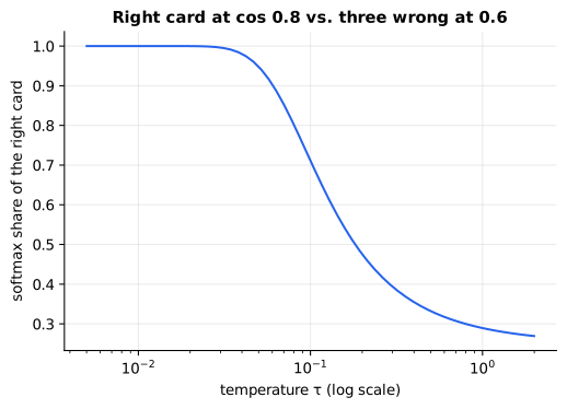
Reading it: the horizontal axis is τ (log scale), the vertical axis is the right card's softmax share when it beats three wrong cards by 0.2 in cosine. At τ = 1 a 0.2 lead earns under a third of the share, so the loss keeps complaining about pairs that are already ranked correctly. Around τ = 0.05 the same lead earns about 95%. Cosines live in a narrow range (−1 to 1), so embedding models use small temperatures (commonly 0.01 to 0.1) to make those small differences count.
In code: positive_probability computes share₊ for given cosines and τ;
this curve is that function swept across τ.
Why it matters: too high a temperature and the model can't become confident; too low and a few hard pairs dominate training and it becomes unstable. It's one of the handful of settings that really matters when fine-tuning an embedding model.
Hard negatives: the experiment
Everyday picture: a driving test on an empty road teaches you to steer. It teaches nothing about merging, because merging never came up. Negatives only teach the distinctions they contain.
The setup (train_bi_encoder): questions come in two intents for each
topic: "how do I fix it?" (answered by a how-to card: "restart, reinstall
and follow the setup guide") and "what are the rules?" (answered by a policy
card: "approval, compliance and usage limits"). The question and answer
cards share almost no words, so matching intent must be learned ("fix"
goes with "restart"), not read off the overlap. Each batch holds one intent
across different topics, so its in-batch negatives differ from the right
card only by topic. We train two identical models; the only difference is
that one also gets each question's same-topic, other-intent card as a hard
negative. Then we test on four topics neither model has seen, including
"password".
flowchart TD
  D[Training pairs] --> A[Batches: one intent,<br/>8 different topics]
  A --> M1[Model 1: in-batch negatives only<br/>wrong cards differ by topic]
  A --> H[Add each question's<br/>look-alike card]
  H --> M2[Model 2: plus hard negatives<br/>wrong cards also differ by intent]
  M1 --> T[Test on unseen topics:<br/>right card vs. look-alike]
  M2 --> T
Reading it: both models see exactly the same questions and answers in the same order. The branch on the right adds one extra wrong card per question, a card that has the right topic but the wrong intent. Both models then take the same exam: for a question about an unseen topic, does the right card beat its look-alike?
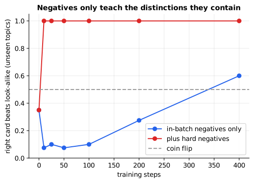
Reading it: the horizontal axis is training steps, the vertical axis is the share of held-out questions whose right card beats the same-topic look-alike (the dashed line is a coin flip). The in-batch-only model spends most of its training below the coin flip, often preferring the wrong card, and ends near 60%. Nothing in its training ever penalised "same topic, wrong intent", so whatever it does on that distinction is an accident of what it learned about topics. With hard negatives the model reaches 100% within ten steps, on topics it never trained on, because it learned what "fix" and "rules" mean.
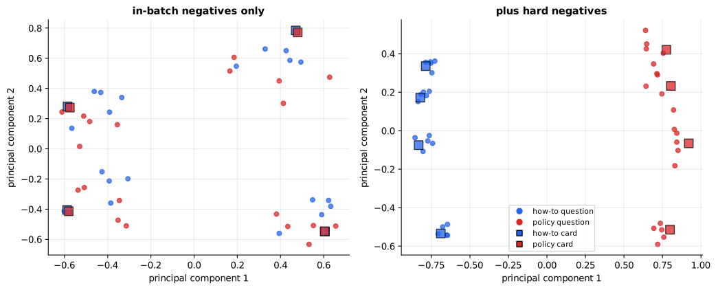
Reading it: each panel squashes the embeddings of the four unseen topics
to 2-D with PCA (the two most spread-out directions; see primer.notation).
Circles are questions and squares are answer cards; blue means how-to and
orange means policy. With in-batch negatives only (left), the points group
by topic, and how-to and policy questions sit on top of each other. With
hard negatives (right), they split by intent, and each question sits next
to the kind of card that actually answers it.
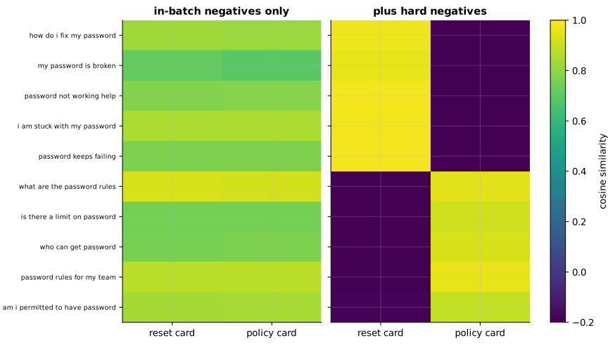
Reading it: rows are the ten "password" questions (five how-to, then five policy), columns are the two password cards, and brighter means a higher cosine. On the left the two columns are nearly the same colour: the model sees "password" and can't tell the cards apart. On the right, the how-to rows light up the reset card and the policy rows light up the policy card: the diagonal blocks are exactly the right answers.
In code: make_pairs builds the (question, right card, look-alike)
triples; look_alike_accuracy runs the exam on unseen topics, and
training_curve records that score at checkpoints during training.
Why it matters: hard negatives are the biggest single driver of retrieval quality. In practice you mine them: search your corpus with BM25 or the current model, and take high-ranking results that are not the right answer.
Fine-tuning on your own domain
flowchart LR
  L[Logs: real questions +<br/>the document that resolved each] --> P[Positive pairs]
  P --> MINE[Mine hard negatives:<br/>top results that are wrong]
  MINE --> T[Fine-tune with InfoNCE,<br/>in-batch + hard negatives]
  T --> E["Evaluate recall@k<br/>on a held-out set"]
  E -->|better than base model| D[Re-embed corpus, deploy]
  E -->|not better| P
Reading it: start from pairs you already have: search logs, support
tickets and the article that closed them, questions and their FAQ entries.
Mine hard negatives from your current search results. Train, then evaluate
recall@k (the share of questions whose right document is in the top k) on
held-out pairs, and only ship if it beats the base model. Shipping means
re-embedding the whole corpus, because a fine-tuned model has a new vector
space (primer.ml.embeddings.operations).
A few thousand good pairs is usually enough to adapt a general model to
legal, medical or internal jargon. Libraries such as sentence-transformers
implement this loss as MultipleNegativesRankingLoss.
CLIP: two encoders, one shared space
Everyday picture: two people describing the same holiday, one through photos and one through postcards. CLIP teaches a photo reader and a text reader to put matching photos and captions at the same spot on one shared map, so a photo of a dog and the words "a photo of a dog" land together.
Tiny example: two images and two captions, each a unit vector. Correctly paired, image 1 scores (1, 0) against the captions and caption 1 scores (1, 0) against the images: each direction's loss is ln(1 + 1/e) = 0.313. Swap the captions and every right pair scores 0 against a wrong pair's 1: the loss rises to ln(1 + e) = 1.313.
Level 3: the formula and its symbols
$$ L_{\text{CLIP}} = \tfrac{1}{2}\left(L_{\text{image} \to \text{text}} + L_{\text{text} \to \text{image}}\right) $$
Symbols
| Symbol | Meaning here |
|---|---|
| L_image→text | InfoNCE where each image (a row of the table) must pick its own caption from all captions in the batch |
| L_text→image | the same loss with the roles swapped: each caption (a column) must pick its own image |
| ½( … + … ) | the average of the two directions |
| L_CLIP | the loss both encoders are trained on together |
In words: each image must find its caption and each caption must find its image.
On the example: ½(0.313 + 0.313) = 0.313 correctly paired; ½(1.313 + 1.313) = 1.313 with the captions swapped.
Level 3: in Python
In Python:
import math
# InfoNCE with τ = 1: row i must pick column i
def rows_pick_diagonal(S):
    return -sum(math.log(math.exp(row[i]) / sum(math.exp(s) for s in row))
                for i, row in enumerate(S)) / len(S)
def clip_loss(S):
    # captions picking images
    columns = [list(col) for col in zip(*S)]
    # ½(L_image→text + L_text→image)
    return (rows_pick_diagonal(S) + rows_pick_diagonal(columns)) / 2
# correctly paired
round(clip_loss([[1, 0], [0, 1]]), 3)  # → 0.313
# captions swapped
round(clip_loss([[0, 1], [1, 0]]), 3)  # → 1.313
In code: clip_loss computes L_CLIP by averaging info_nce_loss over the
rows (images pick captions) and the columns (captions pick images).
flowchart LR
  I[Images] --> IE[Image encoder] --> IV[Image vectors]
  T[Captions] --> TE[Text encoder] --> TV[Text vectors]
  IV --> S["Similarity table<br/>(images × captions)"]
  TV --> S
  S --> L[Symmetric InfoNCE:<br/>rows pick captions,<br/>columns pick images]
  Z["'a photo of a {label}'"] --> TE
Reading it: two different encoders, one per modality, each end in vectors of the same length. The similarity table compares every image with every caption in the batch, and the loss runs along the rows and down the columns. The extra input at the bottom left is the zero-shot trick: to classify an image with no extra training, write a caption for each label, embed it, and pick the label whose caption is closest.
train_clip_toy trains two small linear encoders on toy "images" and
"captions" that describe the same hidden meaning through different, unrelated
feature spaces. Before training, zero-shot labeling is near chance (20% for
five classes); after training it's above 90%.
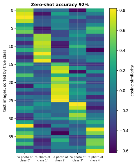
Reading it: rows are 40 test images sorted by their true class, columns are the five label captions, and brighter means more similar. Each block of rows lights up brightest in its own label's column, and that diagonal staircase is zero-shot classification working: no classifier was trained, just two encoders that agree on where meanings live. It isn't perfect. Look for the rows whose brightest cell sits in the wrong column: 4 of these 40 images are closest to another class's caption, three of them classes 0 and 4 mistaken for each other. Over all 500 held-out test images the accuracy is 92%, the number in the figure's title.
Why it matters: the shared space enables search across modalities (find images with text, or text with images), zero-shot classification, and mixing scanned document images with text in one retrieval index. Multimodal models use the same recipe.
In 20 seconds
- Contrastive training pulls matching pairs together and pushes non-matches apart; the loss (InfoNCE) is softmax cross-entropy over the batch.
- In-batch negatives are free: every other answer in the batch.
- Negatives only teach the distinctions they contain. Hard negatives (same topic, wrong answer) are what teach retrieval rather than topic matching.
- Temperature sharpens the softmax so small cosine gaps count; typical τ is 0.01 to 0.1.
- CLIP applies the same loss in both directions between an image encoder and a text encoder, which gives one shared space and zero-shot classification.
Self-test questions
Q: How are embedding models trained? Contrastively, on (query, relevant passage) pairs: an encoder embeds both, and InfoNCE rewards the pair's similarity over the similarity to other passages in the batch (in-batch negatives) and to deliberately chosen hard negatives.
Q: Why do hard negatives matter so much? Random negatives are usually about something else, so a model can beat them by topic matching alone. Hard negatives share the topic but don't answer the question, forcing the model to learn the fine distinction that retrieval actually needs.
Q: What does the temperature do in InfoNCE? It divides the similarities before softmax. A small temperature makes the softmax sharp, so small cosine differences produce large differences in probability and gradient. Too small makes training unstable; too large makes the model unable to become confident.
Q: How does CLIP put images and text in the same space? It trains an image encoder and a text encoder together on image-caption pairs with a symmetric contrastive loss: each image must pick its caption from the batch and each caption must pick its image. Matching pairs end up close in one shared space.
Q: How would you adapt an embedding model to a company's jargon? Collect real (query, correct document) pairs from logs, mine hard negatives from current search results, fine-tune with in-batch plus hard negatives, evaluate recall@k on a held-out set against the base model, then re-embed the corpus with the new model.
The papers behind this lesson
- van den Oord, Li and Vinyals, Representation Learning with Contrastive Predictive Coding (2018): https://arxiv.org/abs/1807.03748. Named and popularised the InfoNCE loss: pick the true sample out of a set of negatives.
- Reimers and Gurevych, Sentence-BERT (2019): https://arxiv.org/abs/1908.10084. Turned BERT into a bi-encoder that produces one comparable vector per sentence, making semantic search with transformers fast. annotated companion
- Karpukhin et al., Dense Passage Retrieval for Open-Domain Question Answering (2020): https://arxiv.org/abs/2004.04906. Showed a question/passage bi-encoder trained with in-batch negatives plus BM25-mined hard negatives beats keyword search for open-domain QA. annotated companion
- Radford et al., Learning Transferable Visual Models From Natural Language Supervision (CLIP, 2021): https://arxiv.org/abs/2103.00020. Trained image and text encoders with a symmetric contrastive loss on 400 million pairs, giving zero-shot image classification. annotated companion
- Gao, Yao and Chen, SimCSE (2021): https://arxiv.org/abs/2104.08821. Showed contrastive learning of sentence embeddings works even with dropout noise as the only "augmentation", and with NLI pairs as hard negatives.
Further reading
- sentence-transformers, training overview: https://www.sbert.net/docs/sentence_transformer/training_overview.html
- Wang et al., Text Embeddings by Weakly-Supervised Contrastive Pre-training (E5, 2022): https://arxiv.org/abs/2212.03533
- Muennighoff et al., MTEB: Massive Text Embedding Benchmark (2022): https://arxiv.org/abs/2210.07316
- MTEB leaderboard: https://huggingface.co/spaces/mteb/leaderboard
- Lilian Weng, Contrastive Representation Learning: https://lilianweng.github.io/posts/2021-05-31-contrastive/
1r""" 2# Contrastive training: how an embedding model learns what "similar" means 3 4Run: `python -m primer.ml.embeddings.contrastive` 5 6New to vectors, dot products, Σ or log? `primer.notation` builds them from zero. 7 8## Level 1: The practitioner's guide 9 10**In one sentence.** Contrastive training teaches an embedding model what 11"similar" means by showing it pairs that belong together and pairs that 12don't, pulling the first kind close and pushing the second apart, and it is 13how nearly every embedding model behind search and RAG was made. 14 15**When you need it.** You need to understand it whenever you pick or judge 16an embedding model, because what a model calls similar is exactly what its 17training pairs called similar: a model trained on (question, answer) pairs 18ranks answers, one trained on (sentence, paraphrase) pairs ranks 19restatements, and neither is "the" similarity. You need to *run* it when a 20general model keeps confusing things your users never confuse: the reset 21steps with the password policy, two product lines that share a name, a 22statute with its commentary. The tell is a retrieval log where the top hit is 23on topic and still wrong. This lesson's experiment puts a number on it: a 24model trained only with random negatives picks the right card over its 25look-alike 60% of the time on unseen topics, barely above a coin flip, 26scoring the reset card at 0.646 and the policy card at 0.632 for "my 27password is broken"; the same model trained with hard negatives picks right 28100% of the time and scores them 0.944 and −0.588. You don't need to train 29anything when a general model already ranks your held-out queries well, and 30you don't need it for one-off comparisons where a person reads the result. 31 32**Your options.** From the cheapest to the most work: 33 34| Option | What it does | What it guarantees | What it costs | Where it lives | 35|---|---|---|---|---| 36| A general pretrained model, as is | Uses vectors from a model trained on millions of public pairs | Good general similarity; on public benchmarks, dense models beat keyword search (DPR: 9 to 19 points of top-20 accuracy over BM25) | Per-token fees or hosting, and nothing about your jargon | An embedding API or an open model | 37| The model's query and document modes | Embeds each side of a search the way the model was trained for it (a query prefix, an input type) | The pairing the model learned, instead of a symmetric comparison it wasn't trained for | Reading the model card | Your embedding calls | 38| Fine-tune with in-batch negatives | Trains on your (query, right document) pairs; every other document in the batch is a free negative | Learns your vocabulary and topics from a few thousand pairs | Pairs from logs, a training run, a full re-embedding of the corpus | Your training job | 39| Fine-tune with mined hard negatives | Adds to each pair a top search result that is wrong | Learns the distinction retrieval needs: right answer versus look-alike | A mining pass over the corpus per training query, plus the above | Your training job | 40| Contrastive pretraining at scale | Trains from weak public pairs before any fine-tuning (E5's CCPairs) | A general model that beats BM25 zero-shot | Curated web-scale pairs and GPU weeks; for model builders | A research lab or a model vendor | 41| Two encoders, one space (CLIP) | Trains an image encoder and a text encoder so matching pairs meet | Search across modalities and zero-shot labelling; 26% to 92% on the lesson's toy | Paired data across modalities (CLIP used 400 million pairs) | A multimodal model | 42 43**How to choose.** Start from what the model must tell apart, and whether it 44already can. 45 46- Measure first: embed a few hundred held-out queries with the general model 47 and check recall@k against the documents that resolved them. Good enough 48 means stop. 49- Check the model card for a query mode before blaming the model; embedding 50 both sides the same way when it expects a prefix costs quality for free. 51- Failures are about vocabulary (your terms, your product names): fine-tune 52 on pairs from logs with in-batch negatives. 53- Failures are about intent (right topic, wrong document): mine hard 54 negatives from your current search results and train with them. This is 55 the step that moved the lesson's model from 60% to 100%. 56- Images, scans or audio next to text: a CLIP-style dual-encoder model, not 57 a text model with captions. 58- Whatever you pick, judge it on held-out pairs against the base model, and 59 ship only a winner. Fine-tuning changes the whole space, so every stored 60 vector is re-embedded. 61 62**What it costs.** Data is the main price, and it is cheap when you have 63logs: real questions and the document that resolved each, support tickets 64and the article that closed them. A few thousand good pairs usually adapt a 65general model to a domain. In-batch negatives are free, which is why batches 66matter: a batch of B pairs gives every question B − 1 negatives at no extra 67cost, and sentence-transformers' guidance for its 68MultipleNegativesRankingLoss is that larger batches are better, with a cached 69variant (GradCache) for large batches on limited memory. Hard negatives cost 70one search per training question, with BM25 or the model itself. Compute for 71fine-tuning is small next to pretraining: the lesson's bi-encoder trains for 72400 steps at batch 8 in seconds, and a fine-tune starts from a model whose 73web-scale training someone else paid for. The recurring bill is deployment: a new model means re-embedding the 74whole corpus, and every model change repeats it. One setting to get right: 75the temperature, the dial that turns small cosine gaps into confident 76scores; typical values are 0.01 to 0.1 (sentence-transformers' default scale 77of 20 is a temperature of 0.05). 78 79**What breaks.** 80 81- **Topic matching instead of answering.** Random negatives are about other 82 subjects, so the model learns subjects: 60% on look-alikes. Mine hard 83 negatives. 84- **A hidden right answer in the batch.** Every card that isn't a question's 85 own is treated as wrong, so two questions with the same answer in one batch 86 push a right answer away. Deduplicate pairs before batching; 87 sentence-transformers' GISTEmbedLoss guides in-batch sampling for this. 88- **Temperature at the wrong setting.** At a temperature of 1, a right card 89 leading three wrong ones by 0.2 in cosine earns only 29% of the softmax, so 90 training keeps punishing correct rankings; at 0.05 it earns 95%. Too low 91 and a few hard pairs dominate and training turns unstable. 92- **Training and testing on the same topics.** The lesson's exam uses four 93 topics the model never saw; a model scored on its training topics looks 94 better than it is. 95- **The old index after a new model.** A fine-tuned model is a new space. 96 Vectors from the old one are not comparable; re-embed everything. 97- **Both sides embedded the same way.** A model trained with a query side and 98 a document side scores worse when you skip the prefix or the input type it 99 was trained with. 100 101**In the wild.** Sentence-BERT (2019) made the bi-encoder the standard 102shape; DPR (2020) trained one on question-passage pairs with in-batch and 103BM25-mined hard negatives and beat BM25 by 9 to 19 points of top-20 accuracy; 104E5 (2022) pretrained contrastively on weakly supervised web pairs and was 105the first to beat BM25 on BEIR with no labels; SimCSE (2021) showed that 106dropout noise alone gives usable positives, with NLI pairs as hard 107negatives; CLIP (2021) trained an image and a text encoder on 400 million 108pairs with the symmetric loss. sentence-transformers implements the loss as 109MultipleNegativesRankingLoss, with CachedMultipleNegativesRankingLoss for big 110batches and GISTEmbedLoss for guided negatives. Cohere's embedding API asks 111which side of a search each text is on. The MTEB leaderboard ranks embedding 112models by the tasks these losses target. 113 114**Go deeper.** Level 2 scores one question against two answer cards by hand, 115turns the scores into a loss (InfoNCE) and shows what the temperature does 116to it, then runs the controlled experiment: two identical models, one with 117hard negatives, tested on topics neither has seen. It ends with the CLIP 118recipe, two encoders trained into one space, and a zero-shot classifier that 119needs no classifier. If you only needed to choose, you are done. 120 121## Level 2: How it works, from scratch 122 123A teacher has a stack of question cards and a stack of answer cards. She 124lays out a few questions, deals out all the answers face up, and asks the 125student to pair each question with its answer. Every wrong pairing, she 126corrects. Over many rounds the student learns what makes an answer fit a 127question. 128 129Then she gets sneaky. Alongside each right answer she slips in a 130**look-alike wrong card**: same subject, wrong answer. "How do I reset my 131password?" now faces both *the reset steps* and *the password policy*. A 132student who only ever saw easy wrong cards (answers about printers or 133holidays) would happily pick the policy card because it says "password". The 134look-alikes force the student to learn the difference that actually matters. 135 136That's **contrastive training**, and it's how nearly every modern embedding 137model is taught. The student is the model; "pairing" means making a 138question's vector point the same way as its answer's vector (see 139`primer.ml.embeddings.similarity`); the wrong cards are **negatives**; the 140look-alikes are **hard negatives**. 141 142## A tiny worked example: one question, two answer cards 143 144A question's vector is q = (1, 0). The right answer is p₊ = (1, 0) and a wrong 145one is p₋ = (0, 1). All three have length 1, so a dot product is a cosine. 146 1471. **Score each card** with the dot product: q·p₊ = 1, q·p₋ = 0. 1482. **Divide by the temperature** τ (tau), a sharpness dial explained 149 below. With τ = 1 the scores stay (1, 0). 1503. **Softmax** (from `primer.ml.attention`): exponentiate and share out. 151 e¹ = 2.718 and e⁰ = 1, so the right card gets 2.718 / 3.718 = **0.731**. 1524. **Loss** = −ln 0.731 = **0.313**. It would be 0 if the right card got 100%. 153 154At τ = 0.1 the scores become (10, 0), the right card gets 99.995%, and the 155loss is **0.0000454**. Same vectors, far more confident: that's what the 156temperature does. 157 158```mermaid 159flowchart LR 160 Q["Question: reset my password"] --> E1[Encoder] 161 P["Right answer: reset steps"] --> E2[Encoder] 162 N["Look-alike: password policy"] --> E3[Encoder] 163 E1 --> PULL[Pull these two<br/>vectors together] 164 E2 --> PULL 165 E1 --> PUSH[Push these two<br/>vectors apart] 166 E3 --> PUSH 167``` 168 169**Reading it:** three texts go through the *same* encoder (the model that 170turns text into a vector). The question and its right answer are pulled 171together; the question and the look-alike are pushed apart. The look-alike 172is about the same topic but doesn't answer the question. Learning to 173separate it from the right answer is what makes a model good at *retrieval* 174(finding the answer) rather than just *topic matching* (finding the subject). 175 176## The math: InfoNCE, the loss behind it 177 178In practice the teacher deals a whole batch. B questions sit in rows, all the 179answer cards in the batch sit in columns, and every card that isn't a 180question's own answer is a free negative for it: **in-batch negatives**. 181 182```mermaid 183flowchart LR 184 subgraph Batch["Similarity table for a batch of 3"] 185 direction TB 186 r1["q₁: ✔ ✗ ✗ | ✗"] 187 r2["q₂: ✗ ✔ ✗ | ✗"] 188 r3["q₃: ✗ ✗ ✔ | ✗"] 189 end 190 Batch --> SM["softmax along<br/>each row"] --> L["loss: −log of the<br/>✔ cell's share"] 191``` 192 193**Reading it:** each row is one question scored against every answer card in 194the batch. The ✔ on the diagonal is its own answer; every ✗ is a negative 195that costs nothing extra because those answers are already in the batch. 196Extra columns to the right of the bar (|) are hard negatives added on purpose, 197which belong to no question. Softmax runs along each row, and the loss asks 198each row to put its share on the ✔. 199 200$$ 201L = -\frac{1}{B}\sum_{i=1}^{B} \log 202\frac{\exp(q_i \cdot p_i / \tau)}{\sum_{j=1}^{M} \exp(q_i \cdot p_j / \tau)} 203$$ 204 205**Symbols** 206 207| Symbol | Meaning here | Shape / range | 208|---|---|---| 209| B | number of questions in the batch | 8 in this lesson | 210| M | number of answer cards in the batch (B, plus any hard negatives) | 8 or 16 here | 211| i | which question (row) | 1 to B | 212| j | which answer card (column) | 1 to M | 213| qᵢ | the i-th question's vector, unit length | d numbers (d = 16) | 214| pᵢ | question i's own answer vector (the ✔) | d numbers | 215| pⱼ | the j-th answer card in the batch | d numbers | 216| · | dot product; equals cosine because the vectors are unit length | −1 to 1 | 217| τ (tau) | temperature: divides every score; small τ sharpens the softmax | 0.01 to 1; 0.1 here | 218| exp | e raised to the power | > 0 | 219| Σⱼ | add up over all M answer cards | | 220| the fraction | softmax share of the right card | 0 to 1 | 221| log, −(1/B) Σᵢ | take −log of each row's share, then average over the rows | L ≥ 0 | 222 223**In words:** for every question, measure what share of its softmax goes to 224its own answer, take the negative log (big when the share is small), and 225average over the batch. 226 227**On the example:** B = 1, M = 2, τ = 1: L = −log(e¹ / (e¹ + e⁰)) = −log 0.731 = 0.313. 228 229**In Python:** 230 231```python 232import math 233def dot(a, b): 234 return sum(a_i * b_i for a_i, b_i in zip(a, b)) 235def info_nce(q, p, tau): 236 B = len(q) 237 total = 0 238 for i in range(B): 239 # exp(q_i · p_j / τ) for every card j 240 exps = [math.exp(dot(q[i], p_j) / tau) for p_j in p] 241 # log of the ✔ card's share 242 total += math.log(exps[i] / sum(exps)) 243 # -(1/B) Σ_i 244 return -total / B 245# B = 1 question 246q = [(1, 0)] 247# M = 2 cards; card 0 is the question's own answer 248p = [(1, 0), (0, 1)] 249round(info_nce(q, p, tau=1), 3) # → 0.313 250print(f"{info_nce(q, p, tau=0.1):.7f}") # → 0.0000454 251``` 252 253The name InfoNCE comes from "noise-contrastive estimation": telling the true 254pair apart from noise. It's the softmax cross-entropy loss from 255`primer.ml.losses`, where the "classes" are the answer cards in the batch. 256 257The model trained here is a deliberately tiny **bi-encoder** (the same 258encoder applied separately to questions and answers): count the words in a 259text (a **bag of words**), multiply by one learned matrix W, and scale the 260result to length 1. `_contrastive_grads` and `_normalize_backward` derive the 261**gradient** (the direction in which each number in W should move to lower 262the loss) by hand, and `encoder_gradient_check` confirms it against a 263brute-force numerical estimate. 264 265**In code:** `info_nce_loss` computes L for a batch, treating any rows of P 266beyond B as extra hard negatives. `BagOfWords` turns text into word counts, 267`BiEncoder` holds the learned matrix W, and `BiEncoder.encode` maps texts to 268unit vectors. 269 270**Why it matters:** the embedding models behind search and RAG (Sentence-BERT, 271DPR, E5 and their successors) are trained with exactly this loss on millions 272of (question, answer) pairs. When a retrieval system confuses "reset my 273password" with "password policy", this is the training signal that was 274missing. 275 276## Temperature: the sharpness dial 277 278**Everyday picture:** grading on a curve. With a gentle curve (high τ), a 279slightly better answer gets slightly more credit. With a steep curve (low τ), 280the best answer takes nearly all the credit, so small differences in score 281become big differences in outcome. 282 283**Tiny example:** the right card has cosine 0.8 and three wrong cards have 2840.6 each. 285 286$$ 287\text{share}_+ = \frac{e^{0.8/\tau}}{e^{0.8/\tau} + 3\,e^{0.6/\tau}} 288$$ 289 290**Symbols** 291 292| Symbol | Meaning here | Range | 293|---|---|---| 294| share₊ | the softmax share that goes to the right card | 0 to 1 | 295| 0.8, 0.6 | cosine of the right card and of each wrong card | −1 to 1 | 296| 3 | the number of (identical) wrong cards | | 297| τ (tau) | temperature: every cosine is divided by it | 0.01 to 1 in practice | 298| e^x | e ≈ 2.718 raised to the power x | > 0 | 299 300**In words:** the right card's share is its exponentiated, temperature-scaled 301score divided by the total over all cards. 302 303**On the example:** at τ = 1, 2.2255 / (2.2255 + 3 × 1.8221) = **0.289**; at τ = 0.05 304the scores become 16 and 12, and 1 / (1 + 3e⁻⁴) = **0.948**. 305 306**In Python:** 307 308```python 309import math 310def share_plus(tau): 311 # e^(0.8/τ) 312 right = math.exp(0.8 / tau) 313 # three wrong cards, e^(0.6/τ) each 314 wrong = 3 * math.exp(0.6 / tau) 315 return right / (right + wrong) 316round(share_plus(1), 3), round(share_plus(0.05), 3) # → (0.289, 0.948) 317``` 318 319 320 321**Reading it:** the horizontal axis is τ (log scale), the vertical axis is 322the right card's softmax share when it beats three wrong cards by 0.2 in 323cosine. At τ = 1 a 0.2 lead earns under a third of the share, so the loss 324keeps complaining about pairs that are already ranked correctly. Around 325τ = 0.05 the same lead earns about 95%. Cosines live in a narrow range (−1 to 3261), so embedding models use small temperatures (commonly 0.01 to 0.1) to 327make those small differences count. 328 329**In code:** `positive_probability` computes share₊ for given cosines and τ; 330this curve is that function swept across τ. 331 332**Why it matters:** too high a temperature and the model can't become 333confident; too low and a few hard pairs dominate training and it becomes 334unstable. It's one of the handful of settings that really matters when 335fine-tuning an embedding model. 336 337## Hard negatives: the experiment 338 339**Everyday picture:** a driving test on an empty road teaches you to steer. 340It teaches nothing about merging, because merging never came up. Negatives 341only teach the distinctions they contain. 342 343**The setup** (`train_bi_encoder`): questions come in two *intents* for each 344topic: "how do I fix it?" (answered by a how-to card: "restart, reinstall 345and follow the setup guide") and "what are the rules?" (answered by a policy 346card: "approval, compliance and usage limits"). The question and answer 347cards share almost no words, so matching intent must be *learned* ("fix" 348goes with "restart"), not read off the overlap. Each batch holds one intent 349across different topics, so its in-batch negatives differ from the right 350card only by topic. We train two identical models; the only difference is 351that one also gets each question's same-topic, other-intent card as a hard 352negative. Then we test on four topics neither model has seen, including 353"password". 354 355```mermaid 356flowchart TD 357 D[Training pairs] --> A[Batches: one intent,<br/>8 different topics] 358 A --> M1[Model 1: in-batch negatives only<br/>wrong cards differ by topic] 359 A --> H[Add each question's<br/>look-alike card] 360 H --> M2[Model 2: plus hard negatives<br/>wrong cards also differ by intent] 361 M1 --> T[Test on unseen topics:<br/>right card vs. look-alike] 362 M2 --> T 363``` 364 365**Reading it:** both models see exactly the same questions and answers in 366the same order. The branch on the right adds one extra wrong card per 367question, a card that has the right topic but the wrong intent. Both models 368then take the same exam: for a question about an unseen topic, does the 369right card beat its look-alike? 370 371 372 373**Reading it:** the horizontal axis is training steps, the vertical axis is 374the share of held-out questions whose right card beats the same-topic 375look-alike (the dashed line is a coin flip). The in-batch-only model spends 376most of its training *below* the coin flip, often preferring the wrong card, 377and ends near 60%. Nothing in its training ever penalised "same topic, wrong 378intent", so whatever it does on that distinction is an accident of what it 379learned about topics. With hard negatives the model reaches 100% within ten 380steps, *on topics it never trained on*, because it learned what "fix" and 381"rules" mean. 382 383 384 385**Reading it:** each panel squashes the embeddings of the four unseen topics 386to 2-D with PCA (the two most spread-out directions; see `primer.notation`). 387Circles are questions and squares are answer cards; blue means how-to and 388orange means policy. With in-batch negatives only (left), the points group 389by *topic*, and how-to and policy questions sit on top of each other. With 390hard negatives (right), they split by *intent*, and each question sits next 391to the kind of card that actually answers it. 392 393 394 395**Reading it:** rows are the ten "password" questions (five how-to, then five 396policy), columns are the two password cards, and brighter means a higher 397cosine. On the left the two columns are nearly the same colour: the model 398sees "password" and can't tell the cards apart. On the right, the how-to 399rows light up the reset card and the policy rows light up the policy card: 400the diagonal blocks are exactly the right answers. 401 402**In code:** `make_pairs` builds the (question, right card, look-alike) 403triples; `look_alike_accuracy` runs the exam on unseen topics, and 404`training_curve` records that score at checkpoints during training. 405 406**Why it matters:** hard negatives are the biggest single driver of 407retrieval quality. In practice you **mine** them: search your corpus with 408BM25 or the current model, and take high-ranking results that are *not* 409the right answer. 410 411## Fine-tuning on your own domain 412 413```mermaid 414flowchart LR 415 L[Logs: real questions +<br/>the document that resolved each] --> P[Positive pairs] 416 P --> MINE[Mine hard negatives:<br/>top results that are wrong] 417 MINE --> T[Fine-tune with InfoNCE,<br/>in-batch + hard negatives] 418 T --> E["Evaluate recall@k<br/>on a held-out set"] 419 E -->|better than base model| D[Re-embed corpus, deploy] 420 E -->|not better| P 421``` 422 423**Reading it:** start from pairs you already have: search logs, support 424tickets and the article that closed them, questions and their FAQ entries. 425Mine hard negatives from your current search results. Train, then evaluate 426recall@k (the share of questions whose right document is in the top k) on 427held-out pairs, and only ship if it beats the base model. Shipping means 428re-embedding the whole corpus, because a fine-tuned model has a new vector 429space (`primer.ml.embeddings.operations`). 430 431A few thousand good pairs is usually enough to adapt a general model to 432legal, medical or internal jargon. Libraries such as sentence-transformers 433implement this loss as `MultipleNegativesRankingLoss`. 434 435## CLIP: two encoders, one shared space 436 437**Everyday picture:** two people describing the same holiday, one through 438photos and one through postcards. CLIP teaches a photo reader and a text 439reader to put matching photos and captions at the same spot on one shared 440map, so a photo of a dog and the words "a photo of a dog" land together. 441 442**Tiny example:** two images and two captions, each a unit vector. 443Correctly paired, image 1 scores (1, 0) against the captions and caption 1 444scores (1, 0) against the images: each direction's loss is ln(1 + 1/e) = 445**0.313**. Swap the captions and every right pair scores 0 against a wrong 446pair's 1: the loss rises to ln(1 + e) = **1.313**. 447 448$$ 449L_{\text{CLIP}} = \tfrac{1}{2}\left(L_{\text{image} \to \text{text}} + L_{\text{text} \to \text{image}}\right) 450$$ 451 452**Symbols** 453 454| Symbol | Meaning here | 455|---|---| 456| L_image→text | InfoNCE where each image (a row of the table) must pick its own caption from all captions in the batch | 457| L_text→image | the same loss with the roles swapped: each caption (a column) must pick its own image | 458| ½( … + … ) | the average of the two directions | 459| L_CLIP | the loss both encoders are trained on together | 460 461**In words:** each image must find its caption *and* each caption must find 462its image. 463 464**On the example:** ½(0.313 + 0.313) = 0.313 correctly paired; ½(1.313 + 1.313) = 4651.313 with the captions swapped. 466 467**In Python:** 468 469```python 470import math 471# InfoNCE with τ = 1: row i must pick column i 472def rows_pick_diagonal(S): 473 return -sum(math.log(math.exp(row[i]) / sum(math.exp(s) for s in row)) 474 for i, row in enumerate(S)) / len(S) 475def clip_loss(S): 476 # captions picking images 477 columns = [list(col) for col in zip(*S)] 478 # ½(L_image→text + L_text→image) 479 return (rows_pick_diagonal(S) + rows_pick_diagonal(columns)) / 2 480# correctly paired 481round(clip_loss([[1, 0], [0, 1]]), 3) # → 0.313 482# captions swapped 483round(clip_loss([[0, 1], [1, 0]]), 3) # → 1.313 484``` 485 486**In code:** `clip_loss` computes L_CLIP by averaging `info_nce_loss` over the 487rows (images pick captions) and the columns (captions pick images). 488 489```mermaid 490flowchart LR 491 I[Images] --> IE[Image encoder] --> IV[Image vectors] 492 T[Captions] --> TE[Text encoder] --> TV[Text vectors] 493 IV --> S["Similarity table<br/>(images × captions)"] 494 TV --> S 495 S --> L[Symmetric InfoNCE:<br/>rows pick captions,<br/>columns pick images] 496 Z["'a photo of a {label}'"] --> TE 497``` 498 499**Reading it:** two different encoders, one per modality, each end in 500vectors of the same length. The similarity table compares every image with 501every caption in the batch, and the loss runs along the rows and down the 502columns. The extra input at the bottom left is the zero-shot trick: to 503classify an image with no extra training, write a caption for each label, 504embed it, and pick the label whose caption is closest. 505 506`train_clip_toy` trains two small linear encoders on toy "images" and 507"captions" that describe the same hidden meaning through different, unrelated 508feature spaces. Before training, zero-shot labeling is near chance (20% for 509five classes); after training it's above 90%. 510 511 512 513**Reading it:** rows are 40 test images sorted by their true class, columns 514are the five label captions, and brighter means more similar. Each block of 515rows lights up brightest in its own label's column, and that diagonal 516staircase is zero-shot classification working: no classifier was trained, 517just two encoders that agree on where meanings live. It isn't perfect. Look 518for the rows whose brightest cell sits in the wrong column: 4 of these 40 519images are closest to another class's caption, three of them classes 0 and 4 520mistaken for each other. Over all 500 held-out test images the accuracy is 52192%, the number in the figure's title. 522 523**Why it matters:** the shared space enables search across modalities 524(find images with text, or text with images), zero-shot classification, 525and mixing scanned document images with text in one retrieval index. 526Multimodal models use the same recipe. 527 528## In 20 seconds 529- Contrastive training pulls matching pairs together and pushes non-matches 530 apart; the loss (InfoNCE) is softmax cross-entropy over the batch. 531- In-batch negatives are free: every other answer in the batch. 532- Negatives only teach the distinctions they contain. Hard negatives (same 533 topic, wrong answer) are what teach retrieval rather than topic matching. 534- Temperature sharpens the softmax so small cosine gaps count; typical τ is 535 0.01 to 0.1. 536- CLIP applies the same loss in both directions between an image encoder and 537 a text encoder, which gives one shared space and zero-shot classification. 538 539## Self-test questions 540 541**Q: How are embedding models trained?** 542Contrastively, on (query, relevant passage) pairs: an encoder embeds both, 543and InfoNCE rewards the pair's similarity over the similarity to other 544passages in the batch (in-batch negatives) and to deliberately chosen hard 545negatives. 546 547**Q: Why do hard negatives matter so much?** 548Random negatives are usually about something else, so a model can beat them 549by topic matching alone. Hard negatives share the topic but don't answer 550the question, forcing the model to learn the fine distinction that 551retrieval actually needs. 552 553**Q: What does the temperature do in InfoNCE?** 554It divides the similarities before softmax. A small temperature makes the 555softmax sharp, so small cosine differences produce large differences in 556probability and gradient. Too small makes training unstable; too large 557makes the model unable to become confident. 558 559**Q: How does CLIP put images and text in the same space?** 560It trains an image encoder and a text encoder together on image-caption 561pairs with a symmetric contrastive loss: each image must pick its caption 562from the batch and each caption must pick its image. Matching pairs end up 563close in one shared space. 564 565**Q: How would you adapt an embedding model to a company's jargon?** 566Collect real (query, correct document) pairs from logs, mine hard negatives 567from current search results, fine-tune with in-batch plus hard negatives, 568evaluate recall@k on a held-out set against the base model, then re-embed 569the corpus with the new model. 570 571## The papers behind this lesson 572 573- **van den Oord, Li and Vinyals, *Representation Learning with Contrastive Predictive Coding* (2018)**: https://arxiv.org/abs/1807.03748. 574 Named and popularised the InfoNCE loss: pick the true sample out of a set of negatives. 575- **Reimers and Gurevych, *Sentence-BERT* (2019)**: https://arxiv.org/abs/1908.10084. 576 Turned BERT into a bi-encoder that produces one comparable vector per sentence, making semantic search with transformers fast. [annotated companion](../../../papers/sentence-bert.html) 577- **Karpukhin et al., *Dense Passage Retrieval for Open-Domain Question Answering* (2020)**: https://arxiv.org/abs/2004.04906. 578 Showed a question/passage bi-encoder trained with in-batch negatives plus BM25-mined hard negatives beats keyword search for open-domain QA. [annotated companion](../../../papers/dpr.html) 579- **Radford et al., *Learning Transferable Visual Models From Natural Language Supervision* (CLIP, 2021)**: https://arxiv.org/abs/2103.00020. 580 Trained image and text encoders with a symmetric contrastive loss on 400 million pairs, giving zero-shot image classification. [annotated companion](../../../papers/clip.html) 581- **Gao, Yao and Chen, *SimCSE* (2021)**: https://arxiv.org/abs/2104.08821. 582 Showed contrastive learning of sentence embeddings works even with dropout noise as the only "augmentation", and with NLI pairs as hard negatives. 583 584## Further reading 585- sentence-transformers, training overview: https://www.sbert.net/docs/sentence_transformer/training_overview.html 586- Wang et al., *Text Embeddings by Weakly-Supervised Contrastive Pre-training* (E5, 2022): https://arxiv.org/abs/2212.03533 587- Muennighoff et al., *MTEB: Massive Text Embedding Benchmark* (2022): https://arxiv.org/abs/2210.07316 588- MTEB leaderboard: https://huggingface.co/spaces/mteb/leaderboard 589- Lilian Weng, *Contrastive Representation Learning*: https://lilianweng.github.io/posts/2021-05-31-contrastive/ 590""" 591 592from __future__ import annotations 593 594from dataclasses import dataclass 595 596import numpy as np 597 598from primer._show import banner, say, table, takeaway 599from primer.common.text import tokenize 600 601# --------------------------------------------------------------------------- 602# 1. The InfoNCE loss, and what the temperature does 603# --------------------------------------------------------------------------- 604 605 606def _log_softmax(S: np.ndarray) -> np.ndarray: 607 S = S - S.max(axis=1, keepdims=True) # subtract the row max so exp() can't overflow 608 return S - np.log(np.exp(S).sum(axis=1, keepdims=True)) 609 610 611def info_nce_loss(Q: np.ndarray, P: np.ndarray, tau: float) -> float: 612 """Mean InfoNCE loss. Row i of Q (a query) should pick row i of P (its passage). 613 614 Q: (B, d) query embeddings. P: (M, d) passage embeddings with M >= B; 615 rows B..M-1 are extra negatives (e.g. hard negatives) that belong to no query. 616 Every other row of P acts as a negative for query i: that's "in-batch negatives". 617 """ 618 S = Q @ P.T / tau # (B, M) scaled similarities; the diagonal holds the true pairs 619 B = Q.shape[0] 620 return float(-_log_softmax(S)[np.arange(B), np.arange(B)].mean()) 621 622 623def positive_probability(pos: float, negs: list[float], tau: float) -> float: 624 """Softmax share the positive gets when its cosine is `pos` and the negatives' are `negs`.""" 625 s = np.array([pos, *negs]) / tau 626 e = np.exp(s - s.max()) 627 return float(e[0] / e.sum()) 628 629 630# --------------------------------------------------------------------------- 631# 2. A tiny bi-encoder: bag of words -> linear projection -> unit vector 632# --------------------------------------------------------------------------- 633 634 635class BagOfWords: 636 """Turns text into a count vector over a fixed vocabulary (one slot per word).""" 637 638 def __init__(self, texts: list[str]): 639 self.vocab = sorted({t for text in texts for t in tokenize(text)}) 640 self.index = {w: i for i, w in enumerate(self.vocab)} 641 642 def __call__(self, texts: list[str]) -> np.ndarray: 643 X = np.zeros((len(texts), len(self.vocab))) 644 for r, text in enumerate(texts): 645 for t in tokenize(text): 646 if t in self.index: 647 X[r, self.index[t]] += 1 648 return X 649 650 651def _normalize_rows(A: np.ndarray) -> tuple[np.ndarray, np.ndarray]: 652 norms = np.linalg.norm(A, axis=1, keepdims=True) + 1e-12 653 return A / norms, norms 654 655 656def _normalize_backward(dU: np.ndarray, U: np.ndarray, norms: np.ndarray) -> np.ndarray: 657 """Gradient through u = a / |a|: remove the part of dU along u, then divide by |a|. 658 659 Changing a along its own direction doesn't change u (it's rescaled away), 660 so only the sideways part of the gradient survives. 661 """ 662 return (dU - U * np.sum(U * dU, axis=1, keepdims=True)) / norms 663 664 665def _contrastive_grads(Q: np.ndarray, P: np.ndarray, tau: float, symmetric: bool = False): 666 """Gradients of the (optionally symmetric) InfoNCE loss w.r.t. Q and P. 667 668 Softmax cross-entropy has a famously simple gradient: probabilities minus 669 the one-hot target. Everything else here is the chain rule through S = Q Pᵀ / τ. 670 """ 671 B, M = Q.shape[0], P.shape[0] 672 S = Q @ P.T / tau 673 Y = np.zeros((B, M)) 674 Y[np.arange(B), np.arange(B)] = 1.0 675 dS = (np.exp(_log_softmax(S)) - Y) / B 676 if symmetric: # CLIP: also each caption picks its image (columns); needs M == B 677 dS = 0.5 * dS + 0.5 * ((np.exp(_log_softmax(S.T)) - Y.T) / B).T 678 return dS @ P / tau, dS.T @ Q / tau 679 680 681@dataclass 682class BiEncoder: 683 """One shared projection W for queries and passages (a "Siamese" bi-encoder).""" 684 685 bow: BagOfWords 686 W: np.ndarray # (vocab, d) 687 688 def encode(self, texts: list[str]) -> np.ndarray: 689 return _normalize_rows(self.bow(texts) @ self.W)[0] 690 691 692def _loss_and_grad(W: np.ndarray, Xq: np.ndarray, Xp: np.ndarray, tau: float) -> tuple[float, np.ndarray]: 693 Aq, Ap = Xq @ W, Xp @ W 694 Q, nq = _normalize_rows(Aq) 695 P, np_ = _normalize_rows(Ap) 696 loss = info_nce_loss(Q, P, tau) 697 dQ, dP = _contrastive_grads(Q, P, tau) 698 dW = Xq.T @ _normalize_backward(dQ, Q, nq) + Xp.T @ _normalize_backward(dP, P, np_) 699 return loss, dW 700 701 702def encoder_gradient_check(seed: int = 0, eps: float = 1e-6) -> float: 703 """Max |analytic - numerical| gradient of the loss w.r.t. W on random data.""" 704 rng = np.random.default_rng(seed) 705 Xq, Xp = rng.random((3, 6)), rng.random((5, 6)) 706 W = rng.standard_normal((6, 4)) 707 _, dW = _loss_and_grad(W, Xq, Xp, 0.5) 708 worst = 0.0 709 for idx in np.ndindex(W.shape): 710 E = np.zeros_like(W) 711 E[idx] = eps 712 num = (_loss_and_grad(W + E, Xq, Xp, 0.5)[0] - _loss_and_grad(W - E, Xq, Xp, 0.5)[0]) / (2 * eps) 713 worst = max(worst, abs(num - dW[idx])) 714 return worst 715 716 717# --------------------------------------------------------------------------- 718# 3. Training data with look-alike passages 719# --------------------------------------------------------------------------- 720 721TRAIN_TOPICS = ["vpn", "laptop", "expense", "pto", "invoice", "printer", "email", "payroll", "badge", "wifi", "travel", "parking"] 722HELDOUT_TOPICS = ["password", "monitor", "phone", "desk"] 723 724# Queries and passages for the same intent share almost no words on purpose, 725# so matching intent has to be *learned* (fix ~ restart), not read off overlap. 726QUERY_TEMPLATES = { 727 "howto": ["how do i fix my {t}", "my {t} is broken", "{t} not working help", "i am stuck with my {t}", "{t} keeps failing"], 728 "policy": ["what are the {t} rules", "is there a limit on {t}", "who can get {t}", "{t} rules for my team", "am i permitted to have {t}"], 729} 730PASSAGE_TEMPLATES = { 731 "howto": "{T}: restart, reinstall and follow the setup guide.", 732 "policy": "{T}: approval, compliance and usage limits for all staff.", 733} 734OTHER = {"howto": "policy", "policy": "howto"} 735 736 737def make_pairs(topics: list[str]) -> list[tuple[str, str, str]]: 738 """(query, right passage, look-alike wrong passage) triples. 739 740 The look-alike has the same topic and the other intent: the classic hard 741 negative ("reset my password" vs. "password policy"). 742 """ 743 out = [] 744 for t in topics: 745 for intent, templates in QUERY_TEMPLATES.items(): 746 for q in templates: 747 out.append( 748 (q.format(t=t), PASSAGE_TEMPLATES[intent].format(T=t.capitalize()), PASSAGE_TEMPLATES[OTHER[intent]].format(T=t.capitalize())) 749 ) 750 return out 751 752 753def train_bi_encoder( 754 hard_negatives: bool, dim: int = 16, tau: float = 0.1, steps: int = 400, batch: int = 8, lr: float = 0.5, seed: int = 0 755) -> BiEncoder: 756 """Train the shared projection with InfoNCE. 757 758 A controlled experiment. Every batch holds one intent (all how-to or all 759 policy questions) across different topics, so its in-batch negatives 760 differ from the right passage *only by topic*. That mirrors real data, 761 where random negatives are nearly always "about something else" and 762 rarely "same subject, different answer". Negatives only teach the 763 distinctions they contain, so this model can succeed by matching topics 764 and never learns intent. With `hard_negatives=True` each query's 765 same-topic, other-intent look-alike is appended to the batch as an extra 766 negative; that is the only difference between the two runs. 767 """ 768 rng = np.random.default_rng(seed) 769 train = make_pairs(TRAIN_TOPICS) 770 everything = train + make_pairs(HELDOUT_TOPICS) 771 bow = BagOfWords([x for triple in everything for x in triple]) 772 W = rng.normal(0, 1 / np.sqrt(dim), (len(bow.vocab), dim)) 773 774 # (topic, intent) -> its triples. Intent is recovered from which passage is "right". 775 groups: dict[tuple[str, str], list] = {} 776 for t in TRAIN_TOPICS: 777 for intent in QUERY_TEMPLATES: 778 right = PASSAGE_TEMPLATES[intent].format(T=t.capitalize()) 779 groups[(t, intent)] = [p for p in train if p[1] == right] 780 for _ in range(steps): 781 intent = ("howto", "policy")[rng.integers(2)] 782 topics = rng.choice(TRAIN_TOPICS, size=batch, replace=False) 783 chosen = [groups[(t, intent)][rng.integers(len(groups[(t, intent)]))] for t in topics] 784 queries = [c[0] for c in chosen] 785 passages = [c[1] for c in chosen] + ([c[2] for c in chosen] if hard_negatives else []) 786 _, dW = _loss_and_grad(W, bow(queries), bow(passages), tau) 787 W -= lr * dW 788 return BiEncoder(bow, W) 789 790 791def look_alike_accuracy(enc: BiEncoder, topics: list[str] = HELDOUT_TOPICS) -> float: 792 """On unseen topics: how often does the right passage beat its same-topic look-alike?""" 793 triples = make_pairs(topics) 794 Q = enc.encode([t[0] for t in triples]) 795 R = enc.encode([t[1] for t in triples]) 796 Wr = enc.encode([t[2] for t in triples]) 797 return float(np.mean(np.sum(Q * R, axis=1) > np.sum(Q * Wr, axis=1))) 798 799 800# --------------------------------------------------------------------------- 801# 4. CLIP: two encoders, one shared space 802# --------------------------------------------------------------------------- 803 804 805def clip_loss(I: np.ndarray, T: np.ndarray, tau: float) -> float: 806 """Symmetric InfoNCE: each image picks its caption AND each caption picks its image.""" 807 I, T = _normalize_rows(I)[0], _normalize_rows(T)[0] 808 return 0.5 * info_nce_loss(I, T, tau) + 0.5 * info_nce_loss(T, I, tau) 809 810 811def train_clip_toy(n_classes: int = 5, dim: int = 16, steps: int = 300, batch: int = 32, tau: float = 0.1, lr: float = 0.5, seed: int = 0) -> dict: 812 """Two linear encoders learn a shared space from (image, caption) pairs. 813 814 Toy data: each example has a hidden meaning z (its class prototype plus 815 noise). The "image" sees z through one random mixing matrix, the "caption" 816 through another, in different sizes, so the raw features live in unrelated 817 spaces. Training aligns them. Zero-shot test: embed one caption per class 818 ("a photo of a <class>", i.e. the clean prototype) and label each held-out 819 image by its nearest caption. 820 """ 821 rng = np.random.default_rng(seed) 822 latent, img_dim, txt_dim = 8, 32, 24 823 protos = rng.standard_normal((n_classes, latent)) 824 A, Bm = rng.standard_normal((latent, img_dim)), rng.standard_normal((latent, txt_dim)) 825 826 def sample(n): 827 y = rng.integers(n_classes, size=n) 828 z = protos[y] + 0.5 * rng.standard_normal((n, latent)) 829 img = z @ A + 0.3 * rng.standard_normal((n, img_dim)) 830 txt = z @ Bm + 0.3 * rng.standard_normal((n, txt_dim)) 831 return img, txt, y 832 833 Wi = rng.normal(0, 1 / np.sqrt(dim), (img_dim, dim)) 834 Wt = rng.normal(0, 1 / np.sqrt(dim), (txt_dim, dim)) 835 for _ in range(steps): 836 img, txt, _ = sample(batch) 837 Ai, At = img @ Wi, txt @ Wt 838 I, ni = _normalize_rows(Ai) 839 T, nt = _normalize_rows(At) 840 dI, dT = _contrastive_grads(I, T, tau, symmetric=True) 841 Wi -= lr * img.T @ _normalize_backward(dI, I, ni) 842 Wt -= lr * txt.T @ _normalize_backward(dT, T, nt) 843 844 test_img, _, test_y = sample(500) 845 label_txt = protos @ Bm # one clean "caption" per class 846 I = _normalize_rows(test_img @ Wi)[0] 847 L = _normalize_rows(label_txt @ Wt)[0] 848 pred = np.argmax(I @ L.T, axis=1) 849 return {"zero_shot_accuracy": float(np.mean(pred == test_y)), "Wi": Wi, "Wt": Wt, "similarity": I[:40] @ L.T, "labels": test_y[:40]} 850 851 852# --------------------------------------------------------------------------- 853# 5. Figures 854# --------------------------------------------------------------------------- 855 856 857def training_curve(hard_negatives: bool, checkpoints=(0, 10, 25, 50, 100, 200, 400)) -> list[float]: 858 """Held-out look-alike accuracy after each number of steps (each a fresh, seeded run).""" 859 return [look_alike_accuracy(train_bi_encoder(hard_negatives, steps=s)) for s in checkpoints] 860 861 862def _pca_2d(X: np.ndarray) -> np.ndarray: 863 Xc = X - X.mean(axis=0) 864 _, _, Vt = np.linalg.svd(Xc, full_matrices=False) 865 return Xc @ Vt[:2].T 866 867 868def figures() -> dict: 869 """Plots computed from this module's own functions. Keys match the docstring's image names.""" 870 import matplotlib 871 872 matplotlib.use("Agg") 873 import matplotlib.pyplot as plt 874 875 figs = {} 876 models = {"in-batch negatives only": train_bi_encoder(False), "plus hard negatives": train_bi_encoder(True)} 877 878 # temperature 879 taus = np.logspace(-2.3, 0.3, 60) 880 fig, ax = plt.subplots(figsize=(5.5, 4)) 881 ax.plot(taus, [positive_probability(0.8, [0.6] * 3, t) for t in taus]) 882 ax.set_xscale("log") 883 ax.set(xlabel="temperature τ (log scale)", ylabel="softmax share of the right card", title="Right card at cos 0.8 vs. three wrong at 0.6") 884 figs["temperature"] = fig 885 886 # training curves 887 cps = (0, 10, 25, 50, 100, 200, 400) 888 fig, ax = plt.subplots(figsize=(5.5, 4)) 889 for hard, label in ((False, "in-batch negatives only"), (True, "plus hard negatives")): 890 ax.plot(cps, training_curve(hard, cps), marker="o", label=label) 891 ax.axhline(0.5, ls="--", color="0.6", label="coin flip") 892 ax.set(xlabel="training steps", ylabel="right card beats look-alike (unseen topics)", ylim=(0, 1.05), title="Negatives only teach the distinctions they contain") 893 ax.legend() 894 figs["training"] = fig 895 896 # space: PCA of held-out questions and cards, coloured by intent 897 triples = make_pairs(HELDOUT_TOPICS) 898 queries = [t[0] for t in triples] 899 q_intent = ["howto" if t[1].endswith("setup guide.") else "policy" for t in triples] 900 cards = sorted({t[1] for t in triples}) 901 c_intent = ["howto" if c.endswith("setup guide.") else "policy" for c in cards] 902 fig, axes = plt.subplots(1, 2, figsize=(11, 4.5)) 903 for ax, (title, enc) in zip(axes, models.items()): 904 P = _pca_2d(enc.encode(queries + cards)) 905 for pts, intents, marker, size in ((P[: len(queries)], q_intent, "o", 25), (P[len(queries) :], c_intent, "s", 90)): 906 for intent, color in (("howto", "C0"), ("policy", "C1")): 907 m = np.array(intents) == intent 908 ax.scatter(pts[m, 0], pts[m, 1], marker=marker, s=size, color=color, alpha=0.75, edgecolor="k" if marker == "s" else None) 909 ax.set(title=title, xlabel="principal component 1", ylabel="principal component 2") 910 handles = [ 911 plt.Line2D([], [], marker="o", ls="", color="C0", label="how-to question"), 912 plt.Line2D([], [], marker="o", ls="", color="C1", label="policy question"), 913 plt.Line2D([], [], marker="s", ls="", color="C0", mec="k", label="how-to card"), 914 plt.Line2D([], [], marker="s", ls="", color="C1", mec="k", label="policy card"), 915 ] 916 axes[1].legend(handles=handles, loc="best", fontsize=8) 917 figs["space"] = fig 918 919 # heatmap: password questions x password cards 920 pw = make_pairs(["password"]) 921 pw_q = [t[0] for t in pw] 922 pw_cards = [PASSAGE_TEMPLATES["howto"].format(T="Password"), PASSAGE_TEMPLATES["policy"].format(T="Password")] 923 # Both panels ask the same questions, so they share one set of row labels on the left. 924 fig, axes = plt.subplots(1, 2, figsize=(9, 5), sharey=True, layout="constrained") 925 for ax, (title, enc) in zip(axes, models.items()): 926 S = enc.encode(pw_q) @ enc.encode(pw_cards).T 927 im = ax.imshow(S, cmap="viridis", vmin=-0.2, vmax=1.0, aspect="auto") 928 ax.set_xticks([0, 1], ["reset card", "policy card"]) 929 ax.set_yticks(range(len(pw_q)), pw_q, fontsize=7) 930 ax.set(title=title) 931 axes[1].tick_params(labelleft=False) 932 fig.colorbar(im, ax=axes, label="cosine similarity") 933 figs["heatmap"] = fig 934 935 # clip 936 r = train_clip_toy() 937 order = np.argsort(r["labels"], kind="stable") 938 fig, ax = plt.subplots(figsize=(5, 6)) 939 im = ax.imshow(r["similarity"][order], cmap="viridis", aspect="auto") 940 ax.set_xticks(range(5), [f"'a photo of\nclass {k}'" for k in range(5)], fontsize=7) 941 ax.set(ylabel="test images, sorted by true class", title=f"Zero-shot accuracy {r['zero_shot_accuracy']:.0%}") 942 fig.colorbar(im, ax=ax, label="cosine similarity") 943 figs["clip"] = fig 944 945 for name, f in figs.items(): 946 if name != "heatmap": # heatmap uses a shared colorbar across axes, which tight_layout can't place 947 f.tight_layout() 948 return figs 949 950 951# --------------------------------------------------------------------------- 952# 6. Narrated walkthrough 953# --------------------------------------------------------------------------- 954 955 956def demo() -> None: 957 banner("1. Worked example: one question, two answer cards") 958 q, cards = np.array([[1.0, 0.0]]), np.array([[1.0, 0.0], [0.0, 1.0]]) 959 table(["temperature τ", "scores", "share of right card", "InfoNCE loss"], 960 [(t, f"({1 / t:g}, 0)", positive_probability(1.0, [0.0], t), info_nce_loss(q, cards, t)) for t in (1.0, 0.1)], floatfmt=".6f") 961 takeaway("Same vectors, lower temperature: the softmax gets sharper and the loss drops.") 962 963 banner("2. Temperature: right card at cos 0.8, three wrong cards at 0.6") 964 table(["τ", "share of right card"], [(t, positive_probability(0.8, [0.6] * 3, t)) for t in (1.0, 0.5, 0.1, 0.05, 0.02)], floatfmt=".3f") 965 966 banner("3. The hand-written gradient is right") 967 say(f"Max difference from a numerical estimate: {encoder_gradient_check():.1e}.") 968 969 banner("4. Hard negatives: the controlled experiment") 970 say( 971 """ 972 Two identical bi-encoders, same batches. Each batch holds one intent 973 across 8 topics, so in-batch negatives differ only by topic. Model 2 974 also gets each question's same-topic, other-intent card. The test: 975 on 4 unseen topics, does the right card beat its look-alike? 976 """ 977 ) 978 easy, hard = train_bi_encoder(False), train_bi_encoder(True) 979 table(["model", "unseen topics", "training topics"], 980 [("in-batch negatives only", look_alike_accuracy(easy), look_alike_accuracy(easy, TRAIN_TOPICS)), 981 ("plus hard negatives", look_alike_accuracy(hard), look_alike_accuracy(hard, TRAIN_TOPICS))], floatfmt=".2f") 982 texts = ["my password is broken and i am stuck", "Password: restart, reinstall and follow the setup guide.", "Password: approval, compliance and usage limits for all staff."] 983 rows = [] 984 for name, enc in (("in-batch only", easy), ("plus hard negatives", hard)): 985 v = enc.encode(texts) 986 rows.append((name, v[0] @ v[1], v[0] @ v[2])) 987 say(f"Query: '{texts[0]}'") 988 table(["model", "cos to reset card", "cos to policy card"], rows, floatfmt=".3f") 989 takeaway("Negatives only teach the distinctions they contain. Hard negatives teach retrieval, not topic matching.") 990 991 banner("5. CLIP: two encoders, one shared space") 992 say(f"Symmetric loss, 2 pairs, correctly paired: {clip_loss(np.eye(2), np.eye(2), 1.0):.4f}; captions swapped: {clip_loss(np.eye(2), np.eye(2)[::-1], 1.0):.4f}.") 993 before, after = train_clip_toy(steps=0), train_clip_toy() 994 table(["encoders", "zero-shot accuracy (5 classes)"], [("untrained", before["zero_shot_accuracy"]), ("after contrastive training", after["zero_shot_accuracy"])], floatfmt=".2f") 995 takeaway("Label an image by embedding one caption per class and picking the nearest: no classifier training needed.") 996 997 998if __name__ == "__main__": 999 demo()
612def info_nce_loss(Q: np.ndarray, P: np.ndarray, tau: float) -> float:
613    """Mean InfoNCE loss. Row i of Q (a query) should pick row i of P (its passage).
614
615    Q: (B, d) query embeddings. P: (M, d) passage embeddings with M >= B;
616    rows B..M-1 are extra negatives (e.g. hard negatives) that belong to no query.
617    Every other row of P acts as a negative for query i: that's "in-batch negatives".
618    """
619    S = Q @ P.T / tau  # (B, M) scaled similarities; the diagonal holds the true pairs
620    B = Q.shape[0]
621    return float(-_log_softmax(S)[np.arange(B), np.arange(B)].mean())
Mean InfoNCE loss. Row i of Q (a query) should pick row i of P (its passage).
Q: (B, d) query embeddings. P: (M, d) passage embeddings with M >= B; rows B..M-1 are extra negatives (e.g. hard negatives) that belong to no query. Every other row of P acts as a negative for query i: that's "in-batch negatives".
624def positive_probability(pos: float, negs: list[float], tau: float) -> float:
625    """Softmax share the positive gets when its cosine is `pos` and the negatives' are `negs`."""
626    s = np.array([pos, *negs]) / tau
627    e = np.exp(s - s.max())
628    return float(e[0] / e.sum())
Softmax share the positive gets when its cosine is pos and the negatives' are negs.
636class BagOfWords:
637    """Turns text into a count vector over a fixed vocabulary (one slot per word)."""
638
639    def __init__(self, texts: list[str]):
640        self.vocab = sorted({t for text in texts for t in tokenize(text)})
641        self.index = {w: i for i, w in enumerate(self.vocab)}
642
643    def __call__(self, texts: list[str]) -> np.ndarray:
644        X = np.zeros((len(texts), len(self.vocab)))
645        for r, text in enumerate(texts):
646            for t in tokenize(text):
647                if t in self.index:
648                    X[r, self.index[t]] += 1
649        return X
Turns text into a count vector over a fixed vocabulary (one slot per word).
682@dataclass
683class BiEncoder:
684    """One shared projection W for queries and passages (a "Siamese" bi-encoder)."""
685
686    bow: BagOfWords
687    W: np.ndarray  # (vocab, d)
688
689    def encode(self, texts: list[str]) -> np.ndarray:
690        return _normalize_rows(self.bow(texts) @ self.W)[0]
One shared projection W for queries and passages (a "Siamese" bi-encoder).
703def encoder_gradient_check(seed: int = 0, eps: float = 1e-6) -> float:
704    """Max |analytic - numerical| gradient of the loss w.r.t. W on random data."""
705    rng = np.random.default_rng(seed)
706    Xq, Xp = rng.random((3, 6)), rng.random((5, 6))
707    W = rng.standard_normal((6, 4))
708    _, dW = _loss_and_grad(W, Xq, Xp, 0.5)
709    worst = 0.0
710    for idx in np.ndindex(W.shape):
711        E = np.zeros_like(W)
712        E[idx] = eps
713        num = (_loss_and_grad(W + E, Xq, Xp, 0.5)[0] - _loss_and_grad(W - E, Xq, Xp, 0.5)[0]) / (2 * eps)
714        worst = max(worst, abs(num - dW[idx]))
715    return worst
Max |analytic - numerical| gradient of the loss w.r.t. W on random data.
738def make_pairs(topics: list[str]) -> list[tuple[str, str, str]]:
739    """(query, right passage, look-alike wrong passage) triples.
740
741    The look-alike has the same topic and the other intent: the classic hard
742    negative ("reset my password" vs. "password policy").
743    """
744    out = []
745    for t in topics:
746        for intent, templates in QUERY_TEMPLATES.items():
747            for q in templates:
748                out.append(
749                    (q.format(t=t), PASSAGE_TEMPLATES[intent].format(T=t.capitalize()), PASSAGE_TEMPLATES[OTHER[intent]].format(T=t.capitalize()))
750                )
751    return out
(query, right passage, look-alike wrong passage) triples.
The look-alike has the same topic and the other intent: the classic hard negative ("reset my password" vs. "password policy").
754def train_bi_encoder(
755    hard_negatives: bool, dim: int = 16, tau: float = 0.1, steps: int = 400, batch: int = 8, lr: float = 0.5, seed: int = 0
756) -> BiEncoder:
757    """Train the shared projection with InfoNCE.
758
759    A controlled experiment. Every batch holds one intent (all how-to or all
760    policy questions) across different topics, so its in-batch negatives
761    differ from the right passage *only by topic*. That mirrors real data,
762    where random negatives are nearly always "about something else" and
763    rarely "same subject, different answer". Negatives only teach the
764    distinctions they contain, so this model can succeed by matching topics
765    and never learns intent. With `hard_negatives=True` each query's
766    same-topic, other-intent look-alike is appended to the batch as an extra
767    negative; that is the only difference between the two runs.
768    """
769    rng = np.random.default_rng(seed)
770    train = make_pairs(TRAIN_TOPICS)
771    everything = train + make_pairs(HELDOUT_TOPICS)
772    bow = BagOfWords([x for triple in everything for x in triple])
773    W = rng.normal(0, 1 / np.sqrt(dim), (len(bow.vocab), dim))
774
775    # (topic, intent) -> its triples. Intent is recovered from which passage is "right".
776    groups: dict[tuple[str, str], list] = {}
777    for t in TRAIN_TOPICS:
778        for intent in QUERY_TEMPLATES:
779            right = PASSAGE_TEMPLATES[intent].format(T=t.capitalize())
780            groups[(t, intent)] = [p for p in train if p[1] == right]
781    for _ in range(steps):
782        intent = ("howto", "policy")[rng.integers(2)]
783        topics = rng.choice(TRAIN_TOPICS, size=batch, replace=False)
784        chosen = [groups[(t, intent)][rng.integers(len(groups[(t, intent)]))] for t in topics]
785        queries = [c[0] for c in chosen]
786        passages = [c[1] for c in chosen] + ([c[2] for c in chosen] if hard_negatives else [])
787        _, dW = _loss_and_grad(W, bow(queries), bow(passages), tau)
788        W -= lr * dW
789    return BiEncoder(bow, W)
Train the shared projection with InfoNCE.
A controlled experiment. Every batch holds one intent (all how-to or all
policy questions) across different topics, so its in-batch negatives
differ from the right passage only by topic. That mirrors real data,
where random negatives are nearly always "about something else" and
rarely "same subject, different answer". Negatives only teach the
distinctions they contain, so this model can succeed by matching topics
and never learns intent. With hard_negatives=True each query's
same-topic, other-intent look-alike is appended to the batch as an extra
negative; that is the only difference between the two runs.
792def look_alike_accuracy(enc: BiEncoder, topics: list[str] = HELDOUT_TOPICS) -> float:
793    """On unseen topics: how often does the right passage beat its same-topic look-alike?"""
794    triples = make_pairs(topics)
795    Q = enc.encode([t[0] for t in triples])
796    R = enc.encode([t[1] for t in triples])
797    Wr = enc.encode([t[2] for t in triples])
798    return float(np.mean(np.sum(Q * R, axis=1) > np.sum(Q * Wr, axis=1)))
On unseen topics: how often does the right passage beat its same-topic look-alike?
806def clip_loss(I: np.ndarray, T: np.ndarray, tau: float) -> float:
807    """Symmetric InfoNCE: each image picks its caption AND each caption picks its image."""
808    I, T = _normalize_rows(I)[0], _normalize_rows(T)[0]
809    return 0.5 * info_nce_loss(I, T, tau) + 0.5 * info_nce_loss(T, I, tau)
Symmetric InfoNCE: each image picks its caption AND each caption picks its image.
812def train_clip_toy(n_classes: int = 5, dim: int = 16, steps: int = 300, batch: int = 32, tau: float = 0.1, lr: float = 0.5, seed: int = 0) -> dict:
813    """Two linear encoders learn a shared space from (image, caption) pairs.
814
815    Toy data: each example has a hidden meaning z (its class prototype plus
816    noise). The "image" sees z through one random mixing matrix, the "caption"
817    through another, in different sizes, so the raw features live in unrelated
818    spaces. Training aligns them. Zero-shot test: embed one caption per class
819    ("a photo of a <class>", i.e. the clean prototype) and label each held-out
820    image by its nearest caption.
821    """
822    rng = np.random.default_rng(seed)
823    latent, img_dim, txt_dim = 8, 32, 24
824    protos = rng.standard_normal((n_classes, latent))
825    A, Bm = rng.standard_normal((latent, img_dim)), rng.standard_normal((latent, txt_dim))
826
827    def sample(n):
828        y = rng.integers(n_classes, size=n)
829        z = protos[y] + 0.5 * rng.standard_normal((n, latent))
830        img = z @ A + 0.3 * rng.standard_normal((n, img_dim))
831        txt = z @ Bm + 0.3 * rng.standard_normal((n, txt_dim))
832        return img, txt, y
833
834    Wi = rng.normal(0, 1 / np.sqrt(dim), (img_dim, dim))
835    Wt = rng.normal(0, 1 / np.sqrt(dim), (txt_dim, dim))
836    for _ in range(steps):
837        img, txt, _ = sample(batch)
838        Ai, At = img @ Wi, txt @ Wt
839        I, ni = _normalize_rows(Ai)
840        T, nt = _normalize_rows(At)
841        dI, dT = _contrastive_grads(I, T, tau, symmetric=True)
842        Wi -= lr * img.T @ _normalize_backward(dI, I, ni)
843        Wt -= lr * txt.T @ _normalize_backward(dT, T, nt)
844
845    test_img, _, test_y = sample(500)
846    label_txt = protos @ Bm  # one clean "caption" per class
847    I = _normalize_rows(test_img @ Wi)[0]
848    L = _normalize_rows(label_txt @ Wt)[0]
849    pred = np.argmax(I @ L.T, axis=1)
850    return {"zero_shot_accuracy": float(np.mean(pred == test_y)), "Wi": Wi, "Wt": Wt, "similarity": I[:40] @ L.T, "labels": test_y[:40]}
Two linear encoders learn a shared space from (image, caption) pairs.
Toy data: each example has a hidden meaning z (its class prototype plus
noise). The "image" sees z through one random mixing matrix, the "caption"
through another, in different sizes, so the raw features live in unrelated
spaces. Training aligns them. Zero-shot test: embed one caption per class
("a photo of a
858def training_curve(hard_negatives: bool, checkpoints=(0, 10, 25, 50, 100, 200, 400)) -> list[float]:
859    """Held-out look-alike accuracy after each number of steps (each a fresh, seeded run)."""
860    return [look_alike_accuracy(train_bi_encoder(hard_negatives, steps=s)) for s in checkpoints]
Held-out look-alike accuracy after each number of steps (each a fresh, seeded run).
869def figures() -> dict:
870    """Plots computed from this module's own functions. Keys match the docstring's image names."""
871    import matplotlib
872
873    matplotlib.use("Agg")
874    import matplotlib.pyplot as plt
875
876    figs = {}
877    models = {"in-batch negatives only": train_bi_encoder(False), "plus hard negatives": train_bi_encoder(True)}
878
879    # temperature
880    taus = np.logspace(-2.3, 0.3, 60)
881    fig, ax = plt.subplots(figsize=(5.5, 4))
882    ax.plot(taus, [positive_probability(0.8, [0.6] * 3, t) for t in taus])
883    ax.set_xscale("log")
884    ax.set(xlabel="temperature τ (log scale)", ylabel="softmax share of the right card", title="Right card at cos 0.8 vs. three wrong at 0.6")
885    figs["temperature"] = fig
886
887    # training curves
888    cps = (0, 10, 25, 50, 100, 200, 400)
889    fig, ax = plt.subplots(figsize=(5.5, 4))
890    for hard, label in ((False, "in-batch negatives only"), (True, "plus hard negatives")):
891        ax.plot(cps, training_curve(hard, cps), marker="o", label=label)
892    ax.axhline(0.5, ls="--", color="0.6", label="coin flip")
893    ax.set(xlabel="training steps", ylabel="right card beats look-alike (unseen topics)", ylim=(0, 1.05), title="Negatives only teach the distinctions they contain")
894    ax.legend()
895    figs["training"] = fig
896
897    # space: PCA of held-out questions and cards, coloured by intent
898    triples = make_pairs(HELDOUT_TOPICS)
899    queries = [t[0] for t in triples]
900    q_intent = ["howto" if t[1].endswith("setup guide.") else "policy" for t in triples]
901    cards = sorted({t[1] for t in triples})
902    c_intent = ["howto" if c.endswith("setup guide.") else "policy" for c in cards]
903    fig, axes = plt.subplots(1, 2, figsize=(11, 4.5))
904    for ax, (title, enc) in zip(axes, models.items()):
905        P = _pca_2d(enc.encode(queries + cards))
906        for pts, intents, marker, size in ((P[: len(queries)], q_intent, "o", 25), (P[len(queries) :], c_intent, "s", 90)):
907            for intent, color in (("howto", "C0"), ("policy", "C1")):
908                m = np.array(intents) == intent
909                ax.scatter(pts[m, 0], pts[m, 1], marker=marker, s=size, color=color, alpha=0.75, edgecolor="k" if marker == "s" else None)
910        ax.set(title=title, xlabel="principal component 1", ylabel="principal component 2")
911    handles = [
912        plt.Line2D([], [], marker="o", ls="", color="C0", label="how-to question"),
913        plt.Line2D([], [], marker="o", ls="", color="C1", label="policy question"),
914        plt.Line2D([], [], marker="s", ls="", color="C0", mec="k", label="how-to card"),
915        plt.Line2D([], [], marker="s", ls="", color="C1", mec="k", label="policy card"),
916    ]
917    axes[1].legend(handles=handles, loc="best", fontsize=8)
918    figs["space"] = fig
919
920    # heatmap: password questions x password cards
921    pw = make_pairs(["password"])
922    pw_q = [t[0] for t in pw]
923    pw_cards = [PASSAGE_TEMPLATES["howto"].format(T="Password"), PASSAGE_TEMPLATES["policy"].format(T="Password")]
924    # Both panels ask the same questions, so they share one set of row labels on the left.
925    fig, axes = plt.subplots(1, 2, figsize=(9, 5), sharey=True, layout="constrained")
926    for ax, (title, enc) in zip(axes, models.items()):
927        S = enc.encode(pw_q) @ enc.encode(pw_cards).T
928        im = ax.imshow(S, cmap="viridis", vmin=-0.2, vmax=1.0, aspect="auto")
929        ax.set_xticks([0, 1], ["reset card", "policy card"])
930        ax.set_yticks(range(len(pw_q)), pw_q, fontsize=7)
931        ax.set(title=title)
932    axes[1].tick_params(labelleft=False)
933    fig.colorbar(im, ax=axes, label="cosine similarity")
934    figs["heatmap"] = fig
935
936    # clip
937    r = train_clip_toy()
938    order = np.argsort(r["labels"], kind="stable")
939    fig, ax = plt.subplots(figsize=(5, 6))
940    im = ax.imshow(r["similarity"][order], cmap="viridis", aspect="auto")
941    ax.set_xticks(range(5), [f"'a photo of\nclass {k}'" for k in range(5)], fontsize=7)
942    ax.set(ylabel="test images, sorted by true class", title=f"Zero-shot accuracy {r['zero_shot_accuracy']:.0%}")
943    fig.colorbar(im, ax=ax, label="cosine similarity")
944    figs["clip"] = fig
945
946    for name, f in figs.items():
947        if name != "heatmap":  # heatmap uses a shared colorbar across axes, which tight_layout can't place
948            f.tight_layout()
949    return figs
Plots computed from this module's own functions. Keys match the docstring's image names.
957def demo() -> None:
958    banner("1. Worked example: one question, two answer cards")
959    q, cards = np.array([[1.0, 0.0]]), np.array([[1.0, 0.0], [0.0, 1.0]])
960    table(["temperature τ", "scores", "share of right card", "InfoNCE loss"],
961          [(t, f"({1 / t:g}, 0)", positive_probability(1.0, [0.0], t), info_nce_loss(q, cards, t)) for t in (1.0, 0.1)], floatfmt=".6f")
962    takeaway("Same vectors, lower temperature: the softmax gets sharper and the loss drops.")
963
964    banner("2. Temperature: right card at cos 0.8, three wrong cards at 0.6")
965    table(["τ", "share of right card"], [(t, positive_probability(0.8, [0.6] * 3, t)) for t in (1.0, 0.5, 0.1, 0.05, 0.02)], floatfmt=".3f")
966
967    banner("3. The hand-written gradient is right")
968    say(f"Max difference from a numerical estimate: {encoder_gradient_check():.1e}.")
969
970    banner("4. Hard negatives: the controlled experiment")
971    say(
972        """
973        Two identical bi-encoders, same batches. Each batch holds one intent
974        across 8 topics, so in-batch negatives differ only by topic. Model 2
975        also gets each question's same-topic, other-intent card. The test:
976        on 4 unseen topics, does the right card beat its look-alike?
977        """
978    )
979    easy, hard = train_bi_encoder(False), train_bi_encoder(True)
980    table(["model", "unseen topics", "training topics"],
981          [("in-batch negatives only", look_alike_accuracy(easy), look_alike_accuracy(easy, TRAIN_TOPICS)),
982           ("plus hard negatives", look_alike_accuracy(hard), look_alike_accuracy(hard, TRAIN_TOPICS))], floatfmt=".2f")
983    texts = ["my password is broken and i am stuck", "Password: restart, reinstall and follow the setup guide.", "Password: approval, compliance and usage limits for all staff."]
984    rows = []
985    for name, enc in (("in-batch only", easy), ("plus hard negatives", hard)):
986        v = enc.encode(texts)
987        rows.append((name, v[0] @ v[1], v[0] @ v[2]))
988    say(f"Query: '{texts[0]}'")
989    table(["model", "cos to reset card", "cos to policy card"], rows, floatfmt=".3f")
990    takeaway("Negatives only teach the distinctions they contain. Hard negatives teach retrieval, not topic matching.")
991
992    banner("5. CLIP: two encoders, one shared space")
993    say(f"Symmetric loss, 2 pairs, correctly paired: {clip_loss(np.eye(2), np.eye(2), 1.0):.4f}; captions swapped: {clip_loss(np.eye(2), np.eye(2)[::-1], 1.0):.4f}.")
994    before, after = train_clip_toy(steps=0), train_clip_toy()
995    table(["encoders", "zero-shot accuracy (5 classes)"], [("untrained", before["zero_shot_accuracy"]), ("after contrastive training", after["zero_shot_accuracy"])], floatfmt=".2f")
996    takeaway("Label an image by embedding one caption per class and picking the nearest: no classifier training needed.")