primer.ml.embeddings.word2vec
word2vec: learning meaning from the company a word keeps
Run: python -m primer.ml.embeddings.word2vec
New to vectors, dot products or Σ? primer.notation builds them from zero.
Level 1: The practitioner's guide
In one sentence. word2vec turns every word in a body of text into a short list of numbers (its vector) by training it to guess its neighbours, so that words used in the same company land close together and can be compared, averaged and searched with arithmetic.
When you need it. You need word vectors the moment a program has to know
that two different strings mean similar things: matching "laptop" to
"notebook computer" in a search box, grouping support tickets by topic,
feeding words to a classifier as something richer than an id, or finding
which products are "like" a given one from the sentences they appear in. The
tell is a synonym table you maintain by hand, or a keyword search that misses
every rephrasing. You don't need word2vec when a word's meaning depends on
the sentence around it: in this lesson's demo the single static vector for
"bank" sits at cosine 0.52 to the river words and 0.50 to the money words,
halfway between its two senses, where one step of attention over "river bank
fish" takes it to 0.83 on the river side and "bank loan cash" to 0.85 on the
money side. And you don't need it for whole sentences or documents:
averaging word vectors is a rough baseline, but the sentence-embedding models
of primer.ml.embeddings.contrastive were built for that job. Today word2vec
is the idea to understand, and a cheap tool for a vocabulary of your own;
contextual models are the default for text.
Your options. Five ways to get a vector per word, from the cheapest to the most capable:
| Option | What it does | What it guarantees | What it costs | Where it lives |
|---|---|---|---|---|
| Download pretrained vectors (GloVe, word2vec, fastText) | Loads a table trained on billions of words of news, Wikipedia or web text | A good general vocabulary in minutes: Stanford's largest GloVe set covers 2.2 million words at 300 dimensions, from 840 billion tokens | A file of gigabytes; words your field uses differently keep their public meaning | A file you load |
| Count, then compress (PPMI + SVD) | Tallies which words appear near which, keeps the pairs that meet more often than chance, compresses the table | Deterministic, one pass over the text, no training loop to tune | Memory for a vocabulary-by-vocabulary table, which caps the vocabulary | Your code |
| Train skip-gram with negative sampling on your corpus | Plays the guessing game on your own text | Vectors that know your jargon; the analogies of Level 2 on clean data | CPU hours in proportion to the text, and a corpus big enough to see each word in many contexts | A library such as gensim, on your machine |
| Subword vectors (fastText) | Builds each word's vector from the vectors of its character pieces | A vector for words never seen in training, including typos and rare inflections | A bigger model, and pieces shared by unrelated words leak into each other | A library |
| Contextual embeddings (BERT and every model since) | Runs the sentence through a transformer and reads off a fresh vector per word, per sentence | Word senses separated by their context | A forward pass per text, a model to host or an API to pay | A model server or an embedding API |
How to choose. Start from whose words they are and whether context matters.
- General English, a prototype by this afternoon: download pretrained vectors and get on with it.
- Your own vocabulary (product codes, ticket jargon, a legal field): train skip-gram on your own text. It runs on a laptop; the demo here trains on 1,800 sentences in seconds.
- Typos, rare words, or a language with many word forms: fastText, which assembles a vector for any spelling.
- A word whose meaning depends on the sentence, or whole sentences to compare: a contextual model, and the rest of this package.
- Whatever you pick, judge the vectors on your own task, not on analogy puzzles. Level 2's corpus is built from three clean attributes so that king − man + woman lands on queen; your search logs are messier, and they are what counts.
What it costs. Training is cheap, which is the point of the method: negative sampling scores one true pair and k noise words per training example instead of the whole vocabulary. The negative-sampling paper reports k = 5 to 20 as useful for small datasets and 2 to 5 for large ones, an optimized single-machine implementation training on more than 100 billion words in a day, and a 2× to 10× further speed-up from subsampling the most frequent words. This lesson trains 16-dimensional vectors for a 45-word vocabulary in seconds. Storage is a table of vocabulary × dimensions numbers: the 400,000-word, 300-dimension GloVe set is 400,000 × 300 × 4 bytes, about 480 MB as float32. Query time costs nothing: a vector is a table lookup, no model runs. Quality, in the paper's own numbers: 300-dimensional vectors trained on a billion words score about 60% on its analogy test, and the same paper names the settings that matter most as the architecture, the vector size, the subsampling rate and the window.
What breaks.
- One vector, many senses. "bank" at 0.52 to river and 0.50 to money is the whole story: a static table cannot separate senses. Use a contextual model where senses matter.
- Words never seen. A word absent from training has no vector, and libraries drop rare words on purpose (gensim's default keeps words seen at least 5 times). Map unknown words to a shared placeholder, or use fastText.
- Order is invisible. The window records which words were near, not in what order: "not good" and "very good" put "good" in the same company. Sentiment and negation need a model that reads order.
- Frequent words swamp the rest. "the" appears next to everything and teaches nothing; the 3/4 power on the noise distribution and subsampling of frequent words exist to counter it. Skip them in a home-made trainer and the vectors degrade.
- The corpus's prejudices come along. Bolukbasi et al. (2016) found that vectors trained on Google News exhibit gender stereotypes "to a disturbing extent". Audit before any decision about people rests on them.
- Public vectors, private meaning. A pretrained "python" is a snake and a language in whatever balance the web had; your codebase has one meaning. Train on your own text when the two differ.
In the wild. gensim's Word2Vec is the standard Python implementation (defaults: 100 dimensions, window 5, 5 negatives, 5 epochs, min_count 5, and the CBOW variant unless you ask for skip-gram). Stanford publishes GloVe vectors trained on Wikipedia and Gigaword (6 billion tokens, 400,000 words, 50 to 300 dimensions) and on Common Crawl (840 billion tokens, 2.2 million words, 300 dimensions). fastText (Bojanowski et al., 2016) is the subword variant. Levy and Goldberg (2014) showed that skip-gram with negative sampling factorizes a shifted PMI table, so counting and predicting are one family. BERT (2018) is the contextual model that replaced static tables as the default, and every sentence-embedding model since inherits its shape.
Go deeper. Level 2 plays the guessing game by hand on a three-word sentence: the pairs a window makes, the dot product, the sigmoid, one nudge of the vectors, and the gradient that nudge follows. It then trains real vectors on a small corpus, checks king − man + woman = queen, gets the same vectors by counting (PPMI + SVD, GloVe), and shows one attention step turning a static "bank" into a contextual one. If you only needed to choose, you are done.
Level 2: How it works, from scratch
You can learn a lot about a stranger from their friends. If two people keep turning up with the same crowd, they probably have something in common. Linguists put it the same way: "You shall know a word by the company it keeps" (J. R. Firth, 1957). "Coffee" and "tea" both show up next to "cup", "hot" and "morning", so they must be related.
word2vec turns that idea into a game. Every word gets a spot on a map of meaning (a short list of numbers, its vector). The game: looking only at a word's spot, guess which words sit near it in real sentences. Every wrong guess nudges the spots a little. After millions of nudges, words that keep the same company end up in the same neighbourhood, because that's the only way to guess well for all of them.
A tiny worked example: one sentence, one nudge
Step 1, make guessing pairs. Take the sentence "river bank fish" and a window of 1 (look one word left and right). Each word, the center, is paired with each neighbour, its context:
(river, bank), (bank, river), (bank, fish), (fish, bank)
No human labels anything: the text itself says which words appeared together.
Step 2, score a pair. Put everything in 2 dimensions. The center word has vector v = (1, 0), its true context word has u = (0, 1), and one random "noise" word (a word we pretend is a context, to have something to push away) has uₙ = (0, −1). The score of a pair is their dot product (multiply matching positions, add): v·u = 1·0 + 0·1 = 0, and v·uₙ = 0. Zero means "no opinion".
Step 3, turn scores into probabilities with the sigmoid σ(x), which squashes any number into 0 to 1 (σ(0) = 0.5, big positive → near 1, big negative → near 0). The model says the true pair is 50% likely and the noise pair is 50% likely. That's bad: we want ~100% and ~0%.
Step 4, measure the mistake as a loss (a single number that's big when the guesses are bad): −ln σ(0) − ln σ(−0) = 0.693 + 0.693 = 1.386.
Step 5, nudge. Move v a little toward u and away from uₙ, and move u and uₙ a little toward or away from v. With a step size (learning rate) of 0.1 we get v = (1, 0.1), u = (0.05, 1), uₙ = (−0.05, −1). Now v·u = 0.15 and v·uₙ = −0.15: the true pair scores higher, the noise pair lower, and the loss drops to 1.242. Word2vec is this nudge, repeated millions of times.
flowchart LR
  S["river bank fish"] --> W[Slide a window<br/>over each word]
  W --> P["(bank, river)<br/>(bank, fish) ..."]
  P --> T[Raise the score of<br/>each true pair]
  N[Draw k random<br/>noise words] --> T2[Lower the score of<br/>each noise pair]
  T --> U[Nudge the vectors<br/>in each pair]
  T2 --> U
  U -->|next pair| P
Reading it: the sentence becomes (center, context) pairs by a sliding window. Each true pair is a positive example; alongside it we draw a few random words as negatives ("bank" should not predict "throne"). The update pulls true pairs together and pushes noise pairs apart, then moves on to the next pair. The loop at the right is the whole training process.
In code: skipgram_pairs slides the window over a sentence and returns
every (center, context) pair; build_corpus writes the lesson's synthetic
sentences for it to slide over.
The math: skip-gram with negative sampling (SGNS)
Every word has two vectors: vᵥ when it's the center and uᵥ when it's a context. For a center c, its true context o and k noise words n₁ … nₖ:
Level 3: the formula and its symbols
$$ L = -\log \sigma(u_o \cdot v_c) - \sum_{i=1}^{k} \log \sigma(-u_{n_i} \cdot v_c), \qquad \sigma(x) = \frac{1}{1 + e^{-x}} $$
Symbols
| Symbol | Meaning here | Shape / range |
|---|---|---|
| L | the loss for one training pair: how wrong the guesses are | ≥ 0; 0 is perfect |
| c, o | the center word and its true context word | word ids |
| vc | the center word's vector | d numbers (d = 16 in this lesson) |
| uo | the true context word's vector | d numbers |
| nᵢ, u_{nᵢ} | the i-th noise word and its vector | k of them, d numbers each |
| k | how many noise words per true pair | 5 here; 5 to 20 in practice |
| · | dot product | one number |
| σ | sigmoid, squashes a score into a probability | 0 to 1 |
| e | Euler's number, ≈ 2.718 | |
| log | natural logarithm; −log p is large when p is small | |
| Σ | add up over i = 1 … k |
In words: the loss is small when the model gives the true pair a high probability and every noise pair a low one.
On the example: L = −log σ(0) − log σ(−0) = 0.693 + 0.693 = 1.386; after the nudge, −log σ(0.15) − log σ(0.15) = 0.621 + 0.621 = 1.242.
Level 3: in Python
In Python:
import math
def sigma(x):
    # σ(x) = 1 / (1 + e^(-x))
    return 1 / (1 + math.exp(-x))
def dot(a, b):
    return sum(a_i * b_i for a_i, b_i in zip(a, b))
def L(v_c, u_o, noise):
    # -log σ(u_o · v_c)
    return (-math.log(sigma(dot(u_o, v_c)))
            # - Σ_i log σ(-u_ni · v_c)
            - sum(math.log(sigma(-dot(u_n, v_c))) for u_n in noise))
round(L((1, 0), (0, 1), [(0, -1)]), 3)  # → 1.386
# after the nudge
round(L((1, 0.1), (0.05, 1), [(-0.05, -1)]), 3)  # → 1.242
The nudge follows the gradient: for each vector, the direction in which
a small change would increase the loss fastest. We step the opposite way.
For this loss the gradients are short enough to derive by hand
(sgns_grads), using the fact that the slope of −log σ(x) is σ(x) − 1:
Level 3: the formula and its symbols
$$ g_o = \sigma(u_o \cdot v_c) - 1, \quad g_i = \sigma(u_{n_i} \cdot v_c), \quad \frac{\partial L}{\partial v_c} = g_o u_o + \sum_i g_i u_{n_i} $$
Symbols
| Symbol | Meaning here | Range |
|---|---|---|
| g_o | how far the true pair's probability is from 1, as a negative number | −1 to 0 |
| gᵢ | the i-th noise pair's probability, which should be 0 | 0 to 1 |
| ∂L/∂vc | gradient: how the loss changes as each number in vc changes | d numbers |
In words: move the center vector toward the true context in proportion to how wrong that guess was, and away from each noise word in proportion to how much it was wrongly believed.
On the example: g_o = 0.5 − 1 = −0.5 and g₁ = 0.5, so ∂L/∂vc = −0.5·(0, 1) + 0.5·(0, −1) = (0, −1). Stepping against it with learning rate 0.1: vc = (1, 0) − 0.1·(0, −1) = (1, 0.1).
Level 3: in Python
In Python:
import math
def sigma(x):
    return 1 / (1 + math.exp(-x))
v_c, u_o, u_n = (1, 0), (0, 1), (0, -1)
# σ(u_o · v_c) - 1
g_o = sigma(sum(u * v for u, v in zip(u_o, v_c))) - 1
# σ(u_n1 · v_c)
g_1 = sigma(sum(u * v for u, v in zip(u_n, v_c)))
g_o, g_1  # → (-0.5, 0.5)
# ∂L/∂v_c = g_o u_o + Σ_i g_i u_ni
grad = [g_o * o + g_1 * n for o, n in zip(u_o, u_n)]
grad  # → [0.0, -1.0]
# step against it, learning rate 0.1
[v - 0.1 * g for v, g in zip(v_c, grad)]  # → [1.0, 0.1]
Noise words are drawn in proportion to their count raised to the 3/4 power:
Level 3: the formula and its symbols
$$ P(w) = \frac{\text{count}(w)^{0.75}}{\sum_{w'} \text{count}(w')^{0.75}} $$
Symbols
| Symbol | Meaning here | Range |
|---|---|---|
| P(w) | chance that word w is drawn as a noise word | 0 to 1; all add to 1 |
| count(w) | how many times w appears in the training text | ≥ 1 |
| ^0.75 | raise to the power 3/4, which shrinks big counts more than small ones | |
| w′ | every word in the vocabulary, in turn | |
| Σ over w′ | add up over the whole vocabulary, so the shares sum to 1 |
In words: common words are drawn as noise more often, but the 3/4 power gives rare words a boost.
On an example: counts 1 and 16 become 1^0.75 = 1 and 16^0.75 = 8, so the shares are 1/9 and 8/9 (0.111 and 0.889) instead of 1/17 and 16/17 (0.059 and 0.941).
Level 3: in Python
In Python:
counts = [1, 16]
# count(w)^0.75
weights = [count ** 0.75 for count in counts]
weights  # → [1.0, 8.0]
# divide by Σ over w′ so the shares add to 1
[round(w / sum(weights), 3) for w in weights]  # → [0.111, 0.889]
# without the 3/4 power
[round(c / sum(counts), 3) for c in counts]  # → [0.059, 0.941]
In code: sgns_loss computes L for one center, one context and k noise
words, sgns_update takes one step against the gradient, and
noise_distribution builds P(w). train_sgns runs the whole loop in
mini-batches and returns a WordVectors table; gradient_check confirms the
hand-derived gradients against a numerical estimate.
Why it matters: a full softmax over the vocabulary (primer.ml.attention
explains softmax) would score every word, 100,000 or more, for every
training pair. Negative sampling scores k + 1. That trick is what made
training on billions of words practical in 2013, and the same pull-together,
push-apart shape reappears in every modern embedding model
(primer.ml.embeddings.contrastive).
The famous result: vector arithmetic
Everyday picture: on a street map, "walk two blocks east" is the same walk wherever you start. word2vec's map works the same way: the walk from "man" to "woman" is roughly the same walk as from "king" to "queen", because in both cases the contexts change from he/his to she/her.
Tiny example with made-up 2-D vectors: man = (1, 0), woman = (1, 1), king = (3, 0). Then king − man + woman = (3 − 1 + 1, 0 − 0 + 1) = (3, 1), exactly where queen = (3, 1) would be.
Level 3: the formula and its symbols
$$ \hat{w} = \operatorname*{arg\,max}_{w \notin {a, b, c}} \cos(v_w,\; v_a - v_b + v_c) $$
Symbols
| Symbol | Meaning here |
|---|---|
| a, b, c | the three given words, e.g. king, man, woman |
| v_a − v_b + v_c | start at king, remove the man direction, add the woman direction |
| cos | cosine similarity (primer.ml.embeddings.similarity) |
| arg max over w | the word w that makes the cosine largest |
| w ∉ {a, b, c} | skip the three input words themselves |
| ŵ | the answer |
In words: the answer is the word whose vector points most nearly the same way as king minus man plus woman, not counting those three words.
On the example: v = (3, 1) and queen = (3, 1) point the same way, so the cosine is 1, and queen wins.
Level 3: in Python
In Python:
import math
def cos(a, b):
    dot = sum(a_i * b_i for a_i, b_i in zip(a, b))
    return dot / (math.sqrt(sum(a_i ** 2 for a_i in a)) * math.sqrt(sum(b_i ** 2 for b_i in b)))
v = {"man": (1, 0), "woman": (1, 1), "king": (3, 0), "queen": (3, 1)}
a, b, c = "king", "man", "woman"
# v_a - v_b + v_c
target = [x_a - x_b + x_c for x_a, x_b, x_c in zip(v[a], v[b], v[c])]
target  # → [3, 1]
# w ∉ {a, b, c}
candidates = [w for w in v if w not in {a, b, c}]
# arg max of the cosine
w_hat = max(candidates, key=lambda w: cos(v[w], target))
w_hat, round(cos(v[w_hat], target), 2)  # → ('queen', 1.0)
This lesson trains on a small synthetic corpus built from three independent attributes (male/female, royal/common, adult/child), so the effect appears in seconds on a laptop.
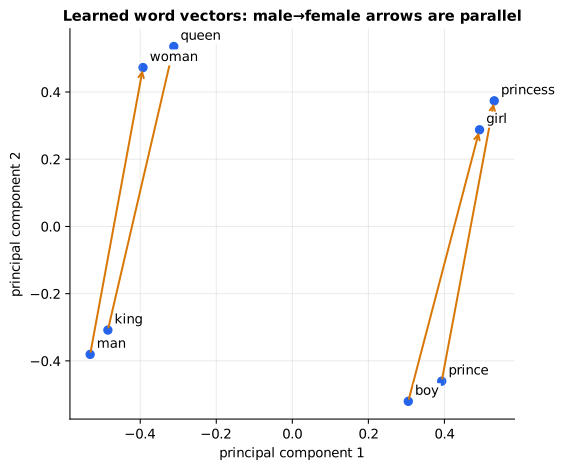
Reading it: these are the learned 16-dimensional vectors, squashed to 2-D
with PCA (a way to find the two directions along which the points are
most spread out, and draw the points along those; primer.notation explains
it). Arrows join male-female pairs: king→queen, man→woman, prince→princess,
boy→girl. The arrows are roughly parallel and about the same length. That
parallelism is the analogy: add the man→woman arrow to king and you land
near queen. The squashing loses some structure, so treat the picture as
intuition, not measurement.
In code: analogy returns the word nearest v_a − v_b + v_c, skipping the
three inputs; nearest lists a word's closest neighbours by cosine, and
nearest_to_vector does the same for any vector.
Why it matters: this was the first clear evidence that learned vectors capture meaning as geometry. It's why "embedding" became the default way to represent text, and why vector arithmetic (averaging, subtracting, finding nearest neighbours) works on meaning.
Counting instead of predicting: PPMI and GloVe
Everyday picture: instead of playing the guessing game, keep a tally sheet: for every pair of words, count how often they appear near each other. Then ask which pairs turn up together more than chance would predict.
Tiny example: two words that each appear only with themselves: counts [[2, 0], [0, 2]]. Out of 4 sightings, each word appears half the time (P = 0.5), and each diagonal pair also appears half the time. Chance would predict 0.5 · 0.5 = 0.25, but we see 0.5, twice as often, so the score is log(0.5 / 0.25) = log 2 = 0.693. The off-diagonal pairs never co-occur, and their score is clipped to 0.
Level 3: the formula and its symbols
$$ \text{PMI}(w, c) = \log \frac{P(w, c)}{P(w)\,P(c)}, \qquad \text{PPMI} = \max(\text{PMI}, 0) $$
Symbols
| Symbol | Meaning here | Range |
|---|---|---|
| w, c | a word and a context word | |
| P(w, c) | share of all co-occurrences that are this pair | 0 to 1 |
| P(w), P(c) | share of co-occurrences involving w (or c) at all | 0 to 1 |
| P(w)P(c) | how often the pair would appear if they were unrelated | |
| log | natural logarithm; log 1 = 0 means "exactly chance" | |
| PMI | pointwise mutual information: log of seen ÷ expected | any; > 0 means "together more than chance" |
| max(·, 0) | keep positive values, replace negatives with 0 |
In words: PMI asks how many times more often two words appear together than they would by chance, on a log scale; PPMI keeps only the "more often" part.
On the example: PMI = log(0.5 / (0.5 · 0.5)) = log 2 = 0.693 on the diagonal; the off-diagonal pairs have P(w, c) = 0, so PMI = −∞ and PPMI = 0.
Level 3: in Python
In Python:
import math
# co-occurrence counts
X = [[2, 0], [0, 2]]
# 4 sightings
total = sum(sum(row) for row in X)
# P(w): share of each row
P_w = [sum(row) / total for row in X]
# P(c): share of each column
P_c = [sum(col) / total for col in zip(*X)]
def ppmi(w, c):
    P_wc = X[w][c] / total
    # log 0 = -∞
    pmi = math.log(P_wc / (P_w[w] * P_c[c])) if P_wc else -math.inf
    # PPMI = max(PMI, 0)
    return max(pmi, 0.0)
[[round(ppmi(w, c), 3) for c in range(2)] for w in range(2)]  # → [[0.693, 0.0], [0.0, 0.693]]
The PPMI table has one row per word, as many columns as the vocabulary, and
is mostly zeros. SVD (singular value decomposition, see primer.notation)
compresses it into a few columns that keep its main patterns; those few
numbers per row are the word's embedding.
flowchart LR
  T[Text] --> C[Count co-occurrences<br/>in a window]
  C --> P[PPMI: keep pairs that meet<br/>more often than chance]
  P --> S[SVD: compress each row<br/>to d numbers]
  S --> E[Word vectors]
Reading it: the same text goes in as for word2vec, but instead of a training loop there are three bulk steps: count, rescale by chance, compress. Levy and Goldberg (2014) showed that word2vec's guessing game is secretly doing the same thing: its vectors factorize a shifted PMI table.
In code: cooccurrence counts the pairs in a window, ppmi rescales the
table by chance and clips negatives to 0, and ppmi_svd_embeddings runs all
three steps and keeps d columns of the SVD.
GloVe (Pennington et al., 2014) is the best-known counting method. It fits vectors so that each dot product predicts the log of the co-occurrence count:
Level 3: the formula and its symbols
$$ w_i \cdot \tilde w_j + b_i + \tilde b_j \approx \log X_{ij} $$
Symbols
| Symbol | Meaning here | Shape |
|---|---|---|
| i, j | two words in the vocabulary | |
| wᵢ | word i's vector | d numbers |
| w̃ⱼ (w-tilde) | word j's vector when it plays the context role | d numbers |
| bᵢ, b̃ⱼ | one extra adjustable number per word (an offset for very common words) | one number each |
| Xᵢⱼ | how many times words i and j appear together | a count |
| log | natural logarithm, which tames huge counts | |
| ≈ | "should be close to"; training shrinks the gap |
In words: two words' vectors should have a dot product (plus offsets) that tells you how often they meet, on a log scale.
On an example: if "ice" and "cold" appear together 20 times, training nudges the vectors until w_ice · w̃_cold + b_ice + b̃_cold ≈ log 20 = 3.0. With 2-D vectors w_ice = (1, 1) and w̃_cold = (1, 0.5) and offsets 0.25 each, the left side is 1.5 + 0.25 + 0.25 = 2.0, still 1.0 short, so training keeps pushing the two vectors to agree more.
Level 3: in Python
In Python:
import math
# log X_ij: the target for 20 co-occurrences
round(math.log(20), 1)  # → 3.0
w_ice, w_cold_tilde = (1, 1), (1, 0.5)
b_ice, b_cold_tilde = 0.25, 0.25
# w_i · w̃_j + b_i + b̃_j
left = sum(a * b for a, b in zip(w_ice, w_cold_tilde)) + b_ice + b_cold_tilde
# the left side, and how far it still falls short
left, round(math.log(20) - left, 1)  # → (2.0, 1.0)
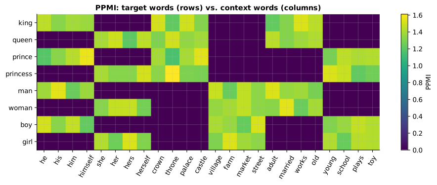
Reading it: rows are the eight target words, columns are the context
words, and brighter cells mean higher PPMI (they meet more than chance). You
can read the attributes straight off the table: the royal words light up
under "crown" and "throne", the female words under "she" and "her", the
children under "young" and "school". SVD compresses exactly these block
patterns into a few directions, and ppmi_svd_embeddings then solves
king − man + woman = queen just like word2vec.
Why it matters: counting and predicting are two routes to the same geometry. That's reassuring: embeddings aren't magic, they're compressed co-occurrence statistics.
The limit: one vector per word
Everyday picture: a phone book lists one address per name. If two different people are called "Bank", the book can only print one address, somewhere between the two. A static embedding table has the same problem: "bank" gets one vector for both the riverbank and the bank account.
Tiny example: after training on this lesson's corpus, the single "bank" vector has cosine about 0.52 with river words and 0.50 with money words: it sits halfway between.
The fix is context. A transformer doesn't look words up once and stop.
It computes a fresh vector for every word in every sentence by attending
over the neighbours (primer.ml.attention): the new vector is a weighted
average of the sentence's vectors,
Level 3: the formula and its symbols
$$ \text{bank}' = \sum_{j} \alpha_j\, x_j, \qquad \sum_j \alpha_j = 1 $$
Symbols
| Symbol | Meaning here | Shape / range |
|---|---|---|
| j | which word of the sentence | 1 to the sentence length |
| xⱼ | the static vector of the j-th word | d numbers |
| αⱼ (alpha) | how much attention "bank" pays to word j (from softmax) | 0 to 1 |
| Σⱼ αⱼ = 1 | the attention weights are shares that add up to 1 | |
| bank′ | the new, context-aware vector for "bank" | d numbers |
In words: the new "bank" is a blend of the sentence's words, weighted by how relevant each one is.
On the example: in "river bank fish", "bank" blends in "river" and "fish", and its cosine with the river words climbs from 0.52 to about 0.83. The same move by hand, in 2-D where the first axis is "river" and the second is "money": river = (1, 0), bank = (1, 1), fish = (1, 0), and α = (0.25, 0.5, 0.25). Then bank′ = 0.25·(1, 0) + 0.5·(1, 1) + 0.25·(1, 0) = (1, 0.5), and its cosine with the river axis climbs from 0.71 to 0.89.
Level 3: in Python
In Python:
import math
# river, bank, fish: axis 1 is "river", axis 2 "money"
x = [(1, 0), (1, 1), (1, 0)]
# attention weights, Σ_j α_j = 1
alpha = [0.25, 0.5, 0.25]
# Σ_j α_j x_j
bank_new = [sum(a_j * x_j[i] for a_j, x_j in zip(alpha, x)) for i in range(2)]
bank_new  # → [1.0, 0.5]
def cos_with_river(v):
    # cosine with (1, 0)
    return v[0] / math.sqrt(v[0] ** 2 + v[1] ** 2)
round(cos_with_river(x[1]), 2), round(cos_with_river(bank_new), 2)  # → (0.71, 0.89)
flowchart LR
  subgraph Static["Static (word2vec, GloVe)"]
    B1["bank"] --> V1["one vector,<br/>both senses blended"]
  end
  subgraph Contextual["Contextual (transformer)"]
    R["river bank fish"] --> A1[attention mixes<br/>in neighbours] --> V2["bank ≈ riverside"]
    M["bank loan cash"] --> A2[attention mixes<br/>in neighbours] --> V3["bank ≈ finance"]
  end
Reading it: on the left a lookup table has one row for "bank", so every
sentence gets the same vector. On the right the same input goes through
attention, which blends in the surrounding words, so the output depends on
the sentence. contextual_bank_demo runs exactly this with the learned
vectors and one attention step.
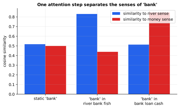
Reading it: bars show cosine similarity to the river sense (probe words water, shore, boat) and to the money sense (money, deposit, account). The static vector is about equally similar to both. After one attention step over "river bank fish" it tilts to the river sense, and over "bank loan cash" it tilts to money. Same word, different vector, decided by context.
Why it matters: this is why BERT (2018) and every embedding model since are built on transformers. Search, RAG and classification all need "Python the language" and "python the snake" to be different points on the map.
In 20 seconds
- word2vec learns a vector per word by guessing nearby words; words that keep the same company get similar vectors.
- Negative sampling makes it cheap: raise the score of the true pair, lower the score of k random pairs, instead of scoring the whole vocabulary.
- Consistent differences in context become consistent directions, hence king − man + woman ≈ queen.
- GloVe and PPMI + SVD count co-occurrences and compress them, and reach the same geometry.
- Static vectors can't separate word senses; contextual (transformer) embeddings can, and they replaced static ones.
Self-test questions
Q: What does skip-gram predict, and where do its training labels come from? Each center word predicts the words within a window around it. The labels come from the text itself (which words actually appeared nearby), so no human labeling is needed.
Q: Why negative sampling instead of a softmax over the vocabulary? A full softmax needs a score for every vocabulary word for every training pair. Negative sampling turns it into k + 1 yes/no decisions (true context vs. a few noise words), which is orders of magnitude cheaper and works as well for learning vectors.
Q: Why does king − man + woman land near queen? The contexts that separate king from queen (he/his vs. she/her) are the same ones that separate man from woman, so training makes those differences the same direction. Adding that direction to "king" moves it toward "queen".
Q: What's the relationship between word2vec and GloVe? Both encode co-occurrence statistics. GloVe explicitly fits log co-occurrence counts; skip-gram with negative sampling implicitly factorizes a shifted PMI matrix. PPMI + SVD gives similar vectors.
Q: What's the main limitation of static word embeddings and what fixed it? One vector per word regardless of meaning, so "bank" blends its senses. Contextual embeddings from transformers compute a vector per word in context, so each sense gets its own representation.
The papers behind this lesson
- Mikolov, Chen, Corrado and Dean, Efficient Estimation of Word Representations in Vector Space (2013), with Mikolov et al., Distributed Representations of Words and Phrases and their Compositionality (2013): https://arxiv.org/abs/1301.3781 and https://arxiv.org/abs/1310.4546. Introduced skip-gram and negative sampling, and the vector-arithmetic analogies. annotated companion
- Pennington, Socher and Manning, GloVe: Global Vectors for Word Representation (2014): https://nlp.stanford.edu/projects/glove/. Fit word vectors directly to log co-occurrence counts, the counting route to the same geometry.
- Levy and Goldberg, Neural Word Embedding as Implicit Matrix Factorization (2014): https://papers.nips.cc/paper/5477-neural-word-embedding-as-implicit-matrix-factorization. Proved that skip-gram with negative sampling implicitly factorizes a shifted PMI matrix, uniting the predicting and counting families.
- Devlin, Chang, Lee and Toutanova, BERT (2018): https://arxiv.org/abs/1810.04805. Made contextual embeddings mainstream: one vector per word per sentence, computed by a transformer.
Further reading
- Mikolov et al., Efficient Estimation of Word Representations in Vector Space (2013): https://arxiv.org/abs/1301.3781
- Mikolov et al., Distributed Representations of Words and Phrases and their Compositionality (negative sampling, 2013): https://arxiv.org/abs/1310.4546
- Goldberg and Levy, word2vec Explained (the gradient derivation): https://arxiv.org/abs/1402.3722
- Levy and Goldberg, Neural Word Embedding as Implicit Matrix Factorization (2014): https://papers.nips.cc/paper/5477-neural-word-embedding-as-implicit-matrix-factorization
- GloVe project page (Stanford NLP): https://nlp.stanford.edu/projects/glove/
- Devlin et al., BERT (contextual embeddings, 2018): https://arxiv.org/abs/1810.04805
- Jay Alammar, The Illustrated Word2vec: https://jalammar.github.io/illustrated-word2vec/
1r""" 2# word2vec: learning meaning from the company a word keeps 3 4Run: `python -m primer.ml.embeddings.word2vec` 5 6New to vectors, dot products or Σ? `primer.notation` builds them from zero. 7 8## Level 1: The practitioner's guide 9 10**In one sentence.** word2vec turns every word in a body of text into a short 11list of numbers (its vector) by training it to guess its neighbours, so that 12words used in the same company land close together and can be compared, 13averaged and searched with arithmetic. 14 15**When you need it.** You need word vectors the moment a program has to know 16that two different strings mean similar things: matching "laptop" to 17"notebook computer" in a search box, grouping support tickets by topic, 18feeding words to a classifier as something richer than an id, or finding 19which products are "like" a given one from the sentences they appear in. The 20tell is a synonym table you maintain by hand, or a keyword search that misses 21every rephrasing. You don't need word2vec when a word's meaning depends on 22the sentence around it: in this lesson's demo the single static vector for 23"bank" sits at cosine 0.52 to the river words and 0.50 to the money words, 24halfway between its two senses, where one step of attention over "river bank 25fish" takes it to 0.83 on the river side and "bank loan cash" to 0.85 on the 26money side. And you don't need it for whole sentences or documents: 27averaging word vectors is a rough baseline, but the sentence-embedding models 28of `primer.ml.embeddings.contrastive` were built for that job. Today word2vec 29is the idea to understand, and a cheap tool for a vocabulary of your own; 30contextual models are the default for text. 31 32**Your options.** Five ways to get a vector per word, from the cheapest to 33the most capable: 34 35| Option | What it does | What it guarantees | What it costs | Where it lives | 36|---|---|---|---|---| 37| Download pretrained vectors (GloVe, word2vec, fastText) | Loads a table trained on billions of words of news, Wikipedia or web text | A good general vocabulary in minutes: Stanford's largest GloVe set covers 2.2 million words at 300 dimensions, from 840 billion tokens | A file of gigabytes; words your field uses differently keep their public meaning | A file you load | 38| Count, then compress (PPMI + SVD) | Tallies which words appear near which, keeps the pairs that meet more often than chance, compresses the table | Deterministic, one pass over the text, no training loop to tune | Memory for a vocabulary-by-vocabulary table, which caps the vocabulary | Your code | 39| Train skip-gram with negative sampling on your corpus | Plays the guessing game on your own text | Vectors that know your jargon; the analogies of Level 2 on clean data | CPU hours in proportion to the text, and a corpus big enough to see each word in many contexts | A library such as gensim, on your machine | 40| Subword vectors (fastText) | Builds each word's vector from the vectors of its character pieces | A vector for words never seen in training, including typos and rare inflections | A bigger model, and pieces shared by unrelated words leak into each other | A library | 41| Contextual embeddings (BERT and every model since) | Runs the sentence through a transformer and reads off a fresh vector per word, per sentence | Word senses separated by their context | A forward pass per text, a model to host or an API to pay | A model server or an embedding API | 42 43**How to choose.** Start from whose words they are and whether context 44matters. 45 46- General English, a prototype by this afternoon: download pretrained 47 vectors and get on with it. 48- Your own vocabulary (product codes, ticket jargon, a legal field): train 49 skip-gram on your own text. It runs on a laptop; the demo here trains on 50 1,800 sentences in seconds. 51- Typos, rare words, or a language with many word forms: fastText, which 52 assembles a vector for any spelling. 53- A word whose meaning depends on the sentence, or whole sentences to 54 compare: a contextual model, and the rest of this package. 55- Whatever you pick, judge the vectors on your own task, not on analogy 56 puzzles. Level 2's corpus is built from three clean attributes so that 57 king − man + woman lands on queen; your search logs are messier, and they 58 are what counts. 59 60**What it costs.** Training is cheap, which is the point of the method: 61negative sampling scores one true pair and k noise words per training 62example instead of the whole vocabulary. The negative-sampling paper reports 63k = 5 to 20 as useful for small datasets and 2 to 5 for large ones, an 64optimized single-machine implementation training on more than 100 billion 65words in a day, and a 2× to 10× further speed-up from subsampling the most 66frequent words. This lesson trains 16-dimensional vectors for a 45-word 67vocabulary in seconds. Storage is a table of vocabulary × dimensions numbers: 68the 400,000-word, 300-dimension GloVe set is 400,000 × 300 × 4 bytes, about 69480 MB as float32. Query time costs nothing: a vector is a table lookup, no 70model runs. Quality, in the paper's own numbers: 300-dimensional vectors 71trained on a billion words score about 60% on its analogy test, and the same 72paper names the settings that matter most as the architecture, the vector 73size, the subsampling rate and the window. 74 75**What breaks.** 76 77- **One vector, many senses.** "bank" at 0.52 to river and 0.50 to money is 78 the whole story: a static table cannot separate senses. Use a contextual 79 model where senses matter. 80- **Words never seen.** A word absent from training has no vector, and 81 libraries drop rare words on purpose (gensim's default keeps words seen at 82 least 5 times). Map unknown words to a shared placeholder, or use fastText. 83- **Order is invisible.** The window records which words were near, not in 84 what order: "not good" and "very good" put "good" in the same company. 85 Sentiment and negation need a model that reads order. 86- **Frequent words swamp the rest.** "the" appears next to everything and 87 teaches nothing; the 3/4 power on the noise distribution and subsampling 88 of frequent words exist to counter it. Skip them in a home-made trainer and 89 the vectors degrade. 90- **The corpus's prejudices come along.** Bolukbasi et al. (2016) found that 91 vectors trained on Google News exhibit gender stereotypes "to a disturbing 92 extent". Audit before any decision about people rests on them. 93- **Public vectors, private meaning.** A pretrained "python" is a snake and a 94 language in whatever balance the web had; your codebase has one meaning. 95 Train on your own text when the two differ. 96 97**In the wild.** gensim's Word2Vec is the standard Python implementation 98(defaults: 100 dimensions, window 5, 5 negatives, 5 epochs, min_count 5, and 99the CBOW variant unless you ask for skip-gram). Stanford publishes GloVe 100vectors trained on Wikipedia and Gigaword (6 billion tokens, 400,000 words, 10150 to 300 dimensions) and on Common Crawl (840 billion tokens, 2.2 million 102words, 300 dimensions). fastText (Bojanowski et al., 2016) is the subword 103variant. Levy and Goldberg (2014) showed that skip-gram with negative 104sampling factorizes a shifted PMI table, so counting and predicting are one 105family. BERT (2018) is the contextual model that replaced static tables as 106the default, and every sentence-embedding model since inherits its shape. 107 108**Go deeper.** Level 2 plays the guessing game by hand on a three-word 109sentence: the pairs a window makes, the dot product, the sigmoid, one nudge 110of the vectors, and the gradient that nudge follows. It then trains real 111vectors on a small corpus, checks king − man + woman = queen, gets the same 112vectors by counting (PPMI + SVD, GloVe), and shows one attention step turning 113a static "bank" into a contextual one. If you only needed to choose, you are 114done. 115 116## Level 2: How it works, from scratch 117 118You can learn a lot about a stranger from their friends. If two people keep 119turning up with the same crowd, they probably have something in common. 120Linguists put it the same way: *"You shall know a word by the company it 121keeps"* (J. R. Firth, 1957). "Coffee" and "tea" both show up next to "cup", 122"hot" and "morning", so they must be related. 123 124word2vec turns that idea into a game. Every word gets a spot on a map of 125meaning (a short list of numbers, its **vector**). The game: looking only at 126a word's spot, guess which words sit near it in real sentences. Every wrong 127guess nudges the spots a little. After millions of nudges, words that keep 128the same company end up in the same neighbourhood, because that's the only 129way to guess well for all of them. 130 131## A tiny worked example: one sentence, one nudge 132 133**Step 1, make guessing pairs.** Take the sentence "river bank fish" and a 134**window** of 1 (look one word left and right). Each word, the **center**, 135is paired with each neighbour, its **context**: 136 137(river, bank), (bank, river), (bank, fish), (fish, bank) 138 139No human labels anything: the text itself says which words appeared together. 140 141**Step 2, score a pair.** Put everything in 2 dimensions. The center word has 142vector v = (1, 0), its true context word has u = (0, 1), and one random 143"noise" word (a word we pretend is a context, to have something to push away) 144has uₙ = (0, −1). The score of a pair is their **dot product** (multiply 145matching positions, add): v·u = 1·0 + 0·1 = 0, and v·uₙ = 0. Zero means "no 146opinion". 147 148**Step 3, turn scores into probabilities** with the **sigmoid** σ(x), which 149squashes any number into 0 to 1 (σ(0) = 0.5, big positive → near 1, big 150negative → near 0). The model says the true pair is 50% likely and the noise 151pair is 50% likely. That's bad: we want ~100% and ~0%. 152 153**Step 4, measure the mistake** as a **loss** (a single number that's big 154when the guesses are bad): −ln σ(0) − ln σ(−0) = 0.693 + 0.693 = **1.386**. 155 156**Step 5, nudge.** Move v a little toward u and away from uₙ, and move u and 157uₙ a little toward or away from v. With a step size (**learning rate**) of 1580.1 we get v = (1, 0.1), u = (0.05, 1), uₙ = (−0.05, −1). Now v·u = **0.15** and 159v·uₙ = **−0.15**: the true pair scores higher, the noise pair lower, and the 160loss drops to **1.242**. Word2vec is this nudge, repeated millions of times. 161 162```mermaid 163flowchart LR 164 S["river bank fish"] --> W[Slide a window<br/>over each word] 165 W --> P["(bank, river)<br/>(bank, fish) ..."] 166 P --> T[Raise the score of<br/>each true pair] 167 N[Draw k random<br/>noise words] --> T2[Lower the score of<br/>each noise pair] 168 T --> U[Nudge the vectors<br/>in each pair] 169 T2 --> U 170 U -->|next pair| P 171``` 172 173**Reading it:** the sentence becomes (center, context) pairs by a sliding 174window. Each true pair is a positive example; alongside it we draw a few 175random words as negatives ("bank" should *not* predict "throne"). The update 176pulls true pairs together and pushes noise pairs apart, then moves on to the 177next pair. The loop at the right is the whole training process. 178 179**In code:** `skipgram_pairs` slides the window over a sentence and returns 180every (center, context) pair; `build_corpus` writes the lesson's synthetic 181sentences for it to slide over. 182 183## The math: skip-gram with negative sampling (SGNS) 184 185Every word has two vectors: vᵥ when it's the center and uᵥ when it's a 186context. For a center c, its true context o and k noise words n₁ … nₖ: 187 188$$ 189L = -\log \sigma(u_o \cdot v_c) - \sum_{i=1}^{k} \log \sigma(-u_{n_i} \cdot v_c), 190\qquad \sigma(x) = \frac{1}{1 + e^{-x}} 191$$ 192 193**Symbols** 194 195| Symbol | Meaning here | Shape / range | 196|---|---|---| 197| L | the loss for one training pair: how wrong the guesses are | ≥ 0; 0 is perfect | 198| c, o | the center word and its true context word | word ids | 199| vc | the center word's vector | d numbers (d = 16 in this lesson) | 200| uo | the true context word's vector | d numbers | 201| nᵢ, u_{nᵢ} | the i-th noise word and its vector | k of them, d numbers each | 202| k | how many noise words per true pair | 5 here; 5 to 20 in practice | 203| · | dot product | one number | 204| σ | sigmoid, squashes a score into a probability | 0 to 1 | 205| e | Euler's number, ≈ 2.718 | | 206| log | natural logarithm; −log p is large when p is small | | 207| Σ | add up over i = 1 … k | | 208 209**In words:** the loss is small when the model gives the true pair a high 210probability and every noise pair a low one. 211 212**On the example:** L = −log σ(0) − log σ(−0) = 0.693 + 0.693 = 1.386; after the 213nudge, −log σ(0.15) − log σ(0.15) = 0.621 + 0.621 = 1.242. 214 215**In Python:** 216 217```python 218import math 219def sigma(x): 220 # σ(x) = 1 / (1 + e^(-x)) 221 return 1 / (1 + math.exp(-x)) 222def dot(a, b): 223 return sum(a_i * b_i for a_i, b_i in zip(a, b)) 224def L(v_c, u_o, noise): 225 # -log σ(u_o · v_c) 226 return (-math.log(sigma(dot(u_o, v_c))) 227 # - Σ_i log σ(-u_ni · v_c) 228 - sum(math.log(sigma(-dot(u_n, v_c))) for u_n in noise)) 229round(L((1, 0), (0, 1), [(0, -1)]), 3) # → 1.386 230# after the nudge 231round(L((1, 0.1), (0.05, 1), [(-0.05, -1)]), 3) # → 1.242 232``` 233 234The nudge follows the **gradient**: for each vector, the direction in which 235a small change would increase the loss fastest. We step the opposite way. 236For this loss the gradients are short enough to derive by hand 237(`sgns_grads`), using the fact that the slope of −log σ(x) is σ(x) − 1: 238 239$$ 240g_o = \sigma(u_o \cdot v_c) - 1, \quad g_i = \sigma(u_{n_i} \cdot v_c), \quad 241\frac{\partial L}{\partial v_c} = g_o u_o + \sum_i g_i u_{n_i} 242$$ 243 244**Symbols** 245 246| Symbol | Meaning here | Range | 247|---|---|---| 248| g_o | how far the true pair's probability is from 1, as a negative number | −1 to 0 | 249| gᵢ | the i-th noise pair's probability, which should be 0 | 0 to 1 | 250| ∂L/∂vc | gradient: how the loss changes as each number in vc changes | d numbers | 251 252**In words:** move the center vector toward the true context in proportion 253to how wrong that guess was, and away from each noise word in proportion to 254how much it was wrongly believed. 255 256**On the example:** g_o = 0.5 − 1 = −0.5 and g₁ = 0.5, so 257∂L/∂vc = −0.5·(0, 1) + 0.5·(0, −1) = (0, −1). Stepping *against* it with learning 258rate 0.1: vc = (1, 0) − 0.1·(0, −1) = (1, 0.1). 259 260**In Python:** 261 262```python 263import math 264def sigma(x): 265 return 1 / (1 + math.exp(-x)) 266v_c, u_o, u_n = (1, 0), (0, 1), (0, -1) 267# σ(u_o · v_c) - 1 268g_o = sigma(sum(u * v for u, v in zip(u_o, v_c))) - 1 269# σ(u_n1 · v_c) 270g_1 = sigma(sum(u * v for u, v in zip(u_n, v_c))) 271g_o, g_1 # → (-0.5, 0.5) 272# ∂L/∂v_c = g_o u_o + Σ_i g_i u_ni 273grad = [g_o * o + g_1 * n for o, n in zip(u_o, u_n)] 274grad # → [0.0, -1.0] 275# step against it, learning rate 0.1 276[v - 0.1 * g for v, g in zip(v_c, grad)] # → [1.0, 0.1] 277``` 278 279Noise words are drawn in proportion to their count raised to the 3/4 power: 280 281$$ 282P(w) = \frac{\text{count}(w)^{0.75}}{\sum_{w'} \text{count}(w')^{0.75}} 283$$ 284 285**Symbols** 286 287| Symbol | Meaning here | Range | 288|---|---|---| 289| P(w) | chance that word w is drawn as a noise word | 0 to 1; all add to 1 | 290| count(w) | how many times w appears in the training text | ≥ 1 | 291| ^0.75 | raise to the power 3/4, which shrinks big counts more than small ones | | 292| w′ | every word in the vocabulary, in turn | | 293| Σ over w′ | add up over the whole vocabulary, so the shares sum to 1 | | 294 295**In words:** common words are drawn as noise more often, but the 3/4 power 296gives rare words a boost. 297 298**On an example:** counts 1 and 16 become 1^0.75 = 1 and 16^0.75 = 8, so the 299shares are 1/9 and 8/9 (0.111 and 0.889) instead of 1/17 and 16/17 (0.059 300and 0.941). 301 302**In Python:** 303 304```python 305counts = [1, 16] 306# count(w)^0.75 307weights = [count ** 0.75 for count in counts] 308weights # → [1.0, 8.0] 309# divide by Σ over w′ so the shares add to 1 310[round(w / sum(weights), 3) for w in weights] # → [0.111, 0.889] 311# without the 3/4 power 312[round(c / sum(counts), 3) for c in counts] # → [0.059, 0.941] 313``` 314 315**In code:** `sgns_loss` computes L for one center, one context and k noise 316words, `sgns_update` takes one step against the gradient, and 317`noise_distribution` builds P(w). `train_sgns` runs the whole loop in 318mini-batches and returns a `WordVectors` table; `gradient_check` confirms the 319hand-derived gradients against a numerical estimate. 320 321**Why it matters:** a full softmax over the vocabulary (`primer.ml.attention` 322explains softmax) would score every word, 100,000 or more, for every 323training pair. Negative sampling scores k + 1. That trick is what made 324training on billions of words practical in 2013, and the same pull-together, 325push-apart shape reappears in every modern embedding model 326(`primer.ml.embeddings.contrastive`). 327 328## The famous result: vector arithmetic 329 330**Everyday picture:** on a street map, "walk two blocks east" is the same 331walk wherever you start. word2vec's map works the same way: the walk from 332"man" to "woman" is roughly the same walk as from "king" to "queen", because 333in both cases the contexts change from he/his to she/her. 334 335**Tiny example** with made-up 2-D vectors: man = (1, 0), woman = (1, 1), 336king = (3, 0). Then king − man + woman = (3 − 1 + 1, 0 − 0 + 1) = (3, 1), exactly 337where queen = (3, 1) would be. 338 339$$ 340\hat{w} = \operatorname*{arg\,max}_{w \notin \{a, b, c\}} \cos(v_w,\; v_a - v_b + v_c) 341$$ 342 343**Symbols** 344 345| Symbol | Meaning here | 346|---|---| 347| a, b, c | the three given words, e.g. king, man, woman | 348| v_a − v_b + v_c | start at king, remove the man direction, add the woman direction | 349| cos | cosine similarity (`primer.ml.embeddings.similarity`) | 350| arg max over w | the word w that makes the cosine largest | 351| w ∉ {a, b, c} | skip the three input words themselves | 352| ŵ | the answer | 353 354**In words:** the answer is the word whose vector points most nearly the 355same way as king minus man plus woman, not counting those three words. 356 357**On the example:** v = (3, 1) and queen = (3, 1) point the same way, so the 358cosine is 1, and queen wins. 359 360**In Python:** 361 362```python 363import math 364def cos(a, b): 365 dot = sum(a_i * b_i for a_i, b_i in zip(a, b)) 366 return dot / (math.sqrt(sum(a_i ** 2 for a_i in a)) * math.sqrt(sum(b_i ** 2 for b_i in b))) 367v = {"man": (1, 0), "woman": (1, 1), "king": (3, 0), "queen": (3, 1)} 368a, b, c = "king", "man", "woman" 369# v_a - v_b + v_c 370target = [x_a - x_b + x_c for x_a, x_b, x_c in zip(v[a], v[b], v[c])] 371target # → [3, 1] 372# w ∉ {a, b, c} 373candidates = [w for w in v if w not in {a, b, c}] 374# arg max of the cosine 375w_hat = max(candidates, key=lambda w: cos(v[w], target)) 376w_hat, round(cos(v[w_hat], target), 2) # → ('queen', 1.0) 377``` 378 379This lesson trains on a small synthetic corpus built from three independent 380attributes (male/female, royal/common, adult/child), so the effect appears 381in seconds on a laptop. 382 383 384 385**Reading it:** these are the learned 16-dimensional vectors, squashed to 2-D 386with **PCA** (a way to find the two directions along which the points are 387most spread out, and draw the points along those; `primer.notation` explains 388it). Arrows join male-female pairs: king→queen, man→woman, prince→princess, 389boy→girl. The arrows are roughly parallel and about the same length. That 390parallelism *is* the analogy: add the man→woman arrow to king and you land 391near queen. The squashing loses some structure, so treat the picture as 392intuition, not measurement. 393 394**In code:** `analogy` returns the word nearest v_a − v_b + v_c, skipping the 395three inputs; `nearest` lists a word's closest neighbours by cosine, and 396`nearest_to_vector` does the same for any vector. 397 398**Why it matters:** this was the first clear evidence that learned vectors 399capture meaning as geometry. It's why "embedding" became the default way to 400represent text, and why vector arithmetic (averaging, subtracting, finding 401nearest neighbours) works on meaning. 402 403## Counting instead of predicting: PPMI and GloVe 404 405**Everyday picture:** instead of playing the guessing game, keep a tally 406sheet: for every pair of words, count how often they appear near each other. 407Then ask which pairs turn up together *more than chance would predict*. 408 409**Tiny example:** two words that each appear only with themselves: 410counts [[2, 0], [0, 2]]. Out of 4 sightings, each word appears half the time 411(P = 0.5), and each diagonal pair also appears half the time. Chance would 412predict 0.5 · 0.5 = 0.25, but we see 0.5, twice as often, so the score is 413log(0.5 / 0.25) = log 2 = **0.693**. The off-diagonal pairs never co-occur, and 414their score is clipped to **0**. 415 416$$ 417\text{PMI}(w, c) = \log \frac{P(w, c)}{P(w)\,P(c)}, \qquad \text{PPMI} = \max(\text{PMI}, 0) 418$$ 419 420**Symbols** 421 422| Symbol | Meaning here | Range | 423|---|---|---| 424| w, c | a word and a context word | | 425| P(w, c) | share of all co-occurrences that are this pair | 0 to 1 | 426| P(w), P(c) | share of co-occurrences involving w (or c) at all | 0 to 1 | 427| P(w)P(c) | how often the pair *would* appear if they were unrelated | | 428| log | natural logarithm; log 1 = 0 means "exactly chance" | | 429| PMI | pointwise mutual information: log of seen ÷ expected | any; > 0 means "together more than chance" | 430| max(·, 0) | keep positive values, replace negatives with 0 | | 431 432**In words:** PMI asks how many times more often two words appear together 433than they would by chance, on a log scale; PPMI keeps only the "more often" 434part. 435 436**On the example:** PMI = log(0.5 / (0.5 · 0.5)) = log 2 = 0.693 on the 437diagonal; the off-diagonal pairs have P(w, c) = 0, so PMI = −∞ and PPMI = 0. 438 439**In Python:** 440 441```python 442import math 443# co-occurrence counts 444X = [[2, 0], [0, 2]] 445# 4 sightings 446total = sum(sum(row) for row in X) 447# P(w): share of each row 448P_w = [sum(row) / total for row in X] 449# P(c): share of each column 450P_c = [sum(col) / total for col in zip(*X)] 451def ppmi(w, c): 452 P_wc = X[w][c] / total 453 # log 0 = -∞ 454 pmi = math.log(P_wc / (P_w[w] * P_c[c])) if P_wc else -math.inf 455 # PPMI = max(PMI, 0) 456 return max(pmi, 0.0) 457[[round(ppmi(w, c), 3) for c in range(2)] for w in range(2)] # → [[0.693, 0.0], [0.0, 0.693]] 458``` 459 460The PPMI table has one row per word, as many columns as the vocabulary, and 461is mostly zeros. **SVD** (singular value decomposition, see `primer.notation`) 462compresses it into a few columns that keep its main patterns; those few 463numbers per row are the word's embedding. 464 465```mermaid 466flowchart LR 467 T[Text] --> C[Count co-occurrences<br/>in a window] 468 C --> P[PPMI: keep pairs that meet<br/>more often than chance] 469 P --> S[SVD: compress each row<br/>to d numbers] 470 S --> E[Word vectors] 471``` 472 473**Reading it:** the same text goes in as for word2vec, but instead of a 474training loop there are three bulk steps: count, rescale by chance, compress. 475Levy and Goldberg (2014) showed that word2vec's guessing game is secretly 476doing the same thing: its vectors factorize a shifted PMI table. 477 478**In code:** `cooccurrence` counts the pairs in a window, `ppmi` rescales the 479table by chance and clips negatives to 0, and `ppmi_svd_embeddings` runs all 480three steps and keeps d columns of the SVD. 481 482**GloVe** (Pennington et al., 2014) is the best-known counting method. It 483fits vectors so that each dot product predicts the log of the co-occurrence 484count: 485 486$$ 487w_i \cdot \tilde w_j + b_i + \tilde b_j \approx \log X_{ij} 488$$ 489 490**Symbols** 491 492| Symbol | Meaning here | Shape | 493|---|---|---| 494| i, j | two words in the vocabulary | | 495| wᵢ | word i's vector | d numbers | 496| w̃ⱼ (w-tilde) | word j's vector when it plays the context role | d numbers | 497| bᵢ, b̃ⱼ | one extra adjustable number per word (an offset for very common words) | one number each | 498| Xᵢⱼ | how many times words i and j appear together | a count | 499| log | natural logarithm, which tames huge counts | | 500| ≈ | "should be close to"; training shrinks the gap | | 501 502**In words:** two words' vectors should have a dot product (plus offsets) 503that tells you how often they meet, on a log scale. 504 505**On an example:** if "ice" and "cold" appear together 20 times, training 506nudges the vectors until w_ice · w̃_cold + b_ice + b̃_cold ≈ log 20 = 3.0. With 5072-D vectors w_ice = (1, 1) and w̃_cold = (1, 0.5) and offsets 0.25 each, the 508left side is 1.5 + 0.25 + 0.25 = 2.0, still 1.0 short, so training keeps 509pushing the two vectors to agree more. 510 511**In Python:** 512 513```python 514import math 515# log X_ij: the target for 20 co-occurrences 516round(math.log(20), 1) # → 3.0 517w_ice, w_cold_tilde = (1, 1), (1, 0.5) 518b_ice, b_cold_tilde = 0.25, 0.25 519# w_i · w̃_j + b_i + b̃_j 520left = sum(a * b for a, b in zip(w_ice, w_cold_tilde)) + b_ice + b_cold_tilde 521# the left side, and how far it still falls short 522left, round(math.log(20) - left, 1) # → (2.0, 1.0) 523``` 524 525 526 527**Reading it:** rows are the eight target words, columns are the context 528words, and brighter cells mean higher PPMI (they meet more than chance). You 529can read the attributes straight off the table: the royal words light up 530under "crown" and "throne", the female words under "she" and "her", the 531children under "young" and "school". SVD compresses exactly these block 532patterns into a few directions, and `ppmi_svd_embeddings` then solves 533king − man + woman = queen just like word2vec. 534 535**Why it matters:** counting and predicting are two routes to the same 536geometry. That's reassuring: embeddings aren't magic, they're compressed 537co-occurrence statistics. 538 539## The limit: one vector per word 540 541**Everyday picture:** a phone book lists one address per name. If two 542different people are called "Bank", the book can only print one address, 543somewhere between the two. A static embedding table has the same problem: 544"bank" gets one vector for both the riverbank and the bank account. 545 546**Tiny example:** after training on this lesson's corpus, the single "bank" 547vector has cosine about 0.52 with river words and 0.50 with money words: it 548sits halfway between. 549 550**The fix is context.** A transformer doesn't look words up once and stop. 551It computes a fresh vector for every word *in every sentence* by attending 552over the neighbours (`primer.ml.attention`): the new vector is a weighted 553average of the sentence's vectors, 554 555$$ 556\text{bank}' = \sum_{j} \alpha_j\, x_j, \qquad \sum_j \alpha_j = 1 557$$ 558 559**Symbols** 560 561| Symbol | Meaning here | Shape / range | 562|---|---|---| 563| j | which word of the sentence | 1 to the sentence length | 564| xⱼ | the static vector of the j-th word | d numbers | 565| αⱼ (alpha) | how much attention "bank" pays to word j (from softmax) | 0 to 1 | 566| Σⱼ αⱼ = 1 | the attention weights are shares that add up to 1 | | 567| bank′ | the new, context-aware vector for "bank" | d numbers | 568 569**In words:** the new "bank" is a blend of the sentence's words, weighted by 570how relevant each one is. 571 572**On the example:** in "river bank fish", "bank" blends in "river" and "fish", 573and its cosine with the river words climbs from 0.52 to about 0.83. The 574same move by hand, in 2-D where the first axis is "river" and the second is 575"money": river = (1, 0), bank = (1, 1), fish = (1, 0), and α = (0.25, 0.5, 0.25). 576Then bank′ = 0.25·(1, 0) + 0.5·(1, 1) + 0.25·(1, 0) = (1, 0.5), and its cosine 577with the river axis climbs from 0.71 to 0.89. 578 579**In Python:** 580 581```python 582import math 583# river, bank, fish: axis 1 is "river", axis 2 "money" 584x = [(1, 0), (1, 1), (1, 0)] 585# attention weights, Σ_j α_j = 1 586alpha = [0.25, 0.5, 0.25] 587# Σ_j α_j x_j 588bank_new = [sum(a_j * x_j[i] for a_j, x_j in zip(alpha, x)) for i in range(2)] 589bank_new # → [1.0, 0.5] 590def cos_with_river(v): 591 # cosine with (1, 0) 592 return v[0] / math.sqrt(v[0] ** 2 + v[1] ** 2) 593round(cos_with_river(x[1]), 2), round(cos_with_river(bank_new), 2) # → (0.71, 0.89) 594``` 595 596```mermaid 597flowchart LR 598 subgraph Static["Static (word2vec, GloVe)"] 599 B1["bank"] --> V1["one vector,<br/>both senses blended"] 600 end 601 subgraph Contextual["Contextual (transformer)"] 602 R["river bank fish"] --> A1[attention mixes<br/>in neighbours] --> V2["bank ≈ riverside"] 603 M["bank loan cash"] --> A2[attention mixes<br/>in neighbours] --> V3["bank ≈ finance"] 604 end 605``` 606 607**Reading it:** on the left a lookup table has one row for "bank", so every 608sentence gets the same vector. On the right the same input goes through 609attention, which blends in the surrounding words, so the output depends on 610the sentence. `contextual_bank_demo` runs exactly this with the learned 611vectors and one attention step. 612 613 614 615**Reading it:** bars show cosine similarity to the river sense (probe words 616water, shore, boat) and to the money sense (money, deposit, account). The 617static vector is about equally similar to both. After one attention step 618over "river bank fish" it tilts to the river sense, and over "bank loan 619cash" it tilts to money. Same word, different vector, decided by context. 620 621**Why it matters:** this is why BERT (2018) and every embedding model since 622are built on transformers. Search, RAG and classification all need 623"Python the language" and "python the snake" to be different points on the 624map. 625 626## In 20 seconds 627- word2vec learns a vector per word by guessing nearby words; words that 628 keep the same company get similar vectors. 629- Negative sampling makes it cheap: raise the score of the true pair, lower 630 the score of k random pairs, instead of scoring the whole vocabulary. 631- Consistent differences in context become consistent directions, hence 632 king − man + woman ≈ queen. 633- GloVe and PPMI + SVD count co-occurrences and compress them, and reach the 634 same geometry. 635- Static vectors can't separate word senses; contextual (transformer) 636 embeddings can, and they replaced static ones. 637 638## Self-test questions 639 640**Q: What does skip-gram predict, and where do its training labels come from?** 641Each center word predicts the words within a window around it. The labels 642come from the text itself (which words actually appeared nearby), so no 643human labeling is needed. 644 645**Q: Why negative sampling instead of a softmax over the vocabulary?** 646A full softmax needs a score for every vocabulary word for every training 647pair. Negative sampling turns it into k + 1 yes/no decisions (true context 648vs. a few noise words), which is orders of magnitude cheaper and works as 649well for learning vectors. 650 651**Q: Why does king − man + woman land near queen?** 652The contexts that separate king from queen (he/his vs. she/her) are the same 653ones that separate man from woman, so training makes those differences the 654same direction. Adding that direction to "king" moves it toward "queen". 655 656**Q: What's the relationship between word2vec and GloVe?** 657Both encode co-occurrence statistics. GloVe explicitly fits log 658co-occurrence counts; skip-gram with negative sampling implicitly factorizes 659a shifted PMI matrix. PPMI + SVD gives similar vectors. 660 661**Q: What's the main limitation of static word embeddings and what fixed it?** 662One vector per word regardless of meaning, so "bank" blends its senses. 663Contextual embeddings from transformers compute a vector per word *in 664context*, so each sense gets its own representation. 665 666## The papers behind this lesson 667 668- **Mikolov, Chen, Corrado and Dean, *Efficient Estimation of Word Representations in Vector Space* (2013)**, with **Mikolov et al., *Distributed Representations of Words and Phrases and their Compositionality* (2013)**: https://arxiv.org/abs/1301.3781 and https://arxiv.org/abs/1310.4546. 669 Introduced skip-gram and negative sampling, and the vector-arithmetic analogies. [annotated companion](../../../papers/word2vec.html) 670- **Pennington, Socher and Manning, *GloVe: Global Vectors for Word Representation* (2014)**: https://nlp.stanford.edu/projects/glove/. 671 Fit word vectors directly to log co-occurrence counts, the counting route to the same geometry. 672- **Levy and Goldberg, *Neural Word Embedding as Implicit Matrix Factorization* (2014)**: https://papers.nips.cc/paper/5477-neural-word-embedding-as-implicit-matrix-factorization. 673 Proved that skip-gram with negative sampling implicitly factorizes a shifted PMI matrix, uniting the predicting and counting families. 674- **Devlin, Chang, Lee and Toutanova, *BERT* (2018)**: https://arxiv.org/abs/1810.04805. 675 Made contextual embeddings mainstream: one vector per word *per sentence*, computed by a transformer. 676 677## Further reading 678- Mikolov et al., *Efficient Estimation of Word Representations in Vector Space* (2013): https://arxiv.org/abs/1301.3781 679- Mikolov et al., *Distributed Representations of Words and Phrases and their Compositionality* (negative sampling, 2013): https://arxiv.org/abs/1310.4546 680- Goldberg and Levy, *word2vec Explained* (the gradient derivation): https://arxiv.org/abs/1402.3722 681- Levy and Goldberg, *Neural Word Embedding as Implicit Matrix Factorization* (2014): https://papers.nips.cc/paper/5477-neural-word-embedding-as-implicit-matrix-factorization 682- GloVe project page (Stanford NLP): https://nlp.stanford.edu/projects/glove/ 683- Devlin et al., *BERT* (contextual embeddings, 2018): https://arxiv.org/abs/1810.04805 684- Jay Alammar, *The Illustrated Word2vec*: https://jalammar.github.io/illustrated-word2vec/ 685""" 686 687from __future__ import annotations 688 689from collections import Counter 690from dataclasses import dataclass 691 692import numpy as np 693 694from primer._show import banner, say, table, takeaway 695from primer.ml.attention import scaled_dot_product_attention 696 697# --------------------------------------------------------------------------- 698# 1. A corpus built so that analogies exist 699# --------------------------------------------------------------------------- 700 701# Eight target words, each a combination of three binary attributes. 702# (gender, status, age) 703TARGETS: dict[str, tuple[str, str, str]] = { 704 "king": ("male", "royal", "adult"), 705 "queen": ("female", "royal", "adult"), 706 "prince": ("male", "royal", "child"), 707 "princess": ("female", "royal", "child"), 708 "man": ("male", "common", "adult"), 709 "woman": ("female", "common", "adult"), 710 "boy": ("male", "common", "child"), 711 "girl": ("female", "common", "child"), 712} 713 714# Each attribute value has its own pool of context words. A target's 715# sentences draw one word from each of its three pools, so its context 716# distribution is the *product* of its attributes. That's the structure 717# vector arithmetic can recover. 718CONTEXT_POOLS: dict[str, list[str]] = { 719 "male": ["he", "his", "him", "himself"], 720 "female": ["she", "her", "hers", "herself"], 721 "royal": ["crown", "throne", "palace", "castle"], 722 "common": ["village", "farm", "market", "street"], 723 "adult": ["adult", "married", "works", "old"], 724 "child": ["young", "school", "plays", "toy"], 725} 726 727# Two senses of "bank", for the one-vector-per-word demo. 728RIVER_WORDS = ["river", "water", "fish", "shore", "boat", "stream"] 729MONEY_WORDS = ["money", "loan", "cash", "deposit", "account", "interest"] 730 731 732def build_corpus(sentences_per_target: int = 150, seed: int = 0) -> list[list[str]]: 733 """Generate short sentences. Deterministic for a given seed.""" 734 rng = np.random.default_rng(seed) 735 corpus: list[list[str]] = [] 736 for word, attrs in TARGETS.items(): 737 for _ in range(sentences_per_target): 738 sent = [word] + [str(rng.choice(CONTEXT_POOLS[a])) for a in attrs] 739 rng.shuffle(sent) 740 corpus.append(sent) 741 # "bank" appears equally often with each sense, so its static vector blends them. 742 for pool in (RIVER_WORDS, MONEY_WORDS): 743 for _ in range(sentences_per_target): 744 corpus.append(["bank"] + [str(w) for w in rng.choice(pool, size=3, replace=False)]) 745 corpus.append([str(w) for w in rng.choice(pool, size=4, replace=False)]) 746 return corpus 747 748 749# --------------------------------------------------------------------------- 750# 2. Training data: (center, context) pairs and the noise distribution 751# --------------------------------------------------------------------------- 752 753 754def skipgram_pairs(sentence: list[str], window: int) -> list[tuple[str, str]]: 755 """Every (center, context) pair with the context at most `window` positions away.""" 756 pairs = [] 757 for i, center in enumerate(sentence): 758 for j in range(max(0, i - window), min(len(sentence), i + window + 1)): 759 if j != i: 760 pairs.append((center, sentence[j])) 761 return pairs 762 763 764def noise_distribution(counts: np.ndarray, power: float = 0.75) -> np.ndarray: 765 """P(noise word) ∝ count^0.75. The power flattens the distribution so 766 rare words are chosen as negatives more often than their raw frequency.""" 767 w = counts.astype(float) ** power 768 return w / w.sum() 769 770 771# --------------------------------------------------------------------------- 772# 3. The SGNS loss and its hand-derived gradients 773# --------------------------------------------------------------------------- 774 775 776def _sigmoid(x: np.ndarray) -> np.ndarray: 777 return 1.0 / (1.0 + np.exp(-x)) 778 779 780def sgns_loss(v_c: np.ndarray, u_o: np.ndarray, u_neg: np.ndarray) -> float: 781 """-log σ(u_o·v_c) - Σ log σ(-u_n·v_c) for one center, one context, k noise words (rows of u_neg).""" 782 return float(-np.log(_sigmoid(u_o @ v_c)) - np.sum(np.log(_sigmoid(-(u_neg @ v_c))))) 783 784 785def sgns_grads(v_c: np.ndarray, u_o: np.ndarray, u_neg: np.ndarray): 786 """Gradients of `sgns_loss` w.r.t. v_c, u_o and each noise vector. 787 788 Derivation: d/dx[-log σ(x)] = σ(x) - 1, and d/dx[-log σ(-x)] = σ(x). 789 Chain rule through x = u·v gives the "g times the other vector" forms. 790 """ 791 g_o = _sigmoid(u_o @ v_c) - 1.0 # negative: pushes u_o·v_c up 792 g_n = _sigmoid(u_neg @ v_c) # positive: pushes u_n·v_c down, shape (k,) 793 d_vc = g_o * u_o + g_n @ u_neg 794 d_uo = g_o * v_c 795 d_un = g_n[:, None] * v_c[None, :] 796 return d_vc, d_uo, d_un 797 798 799def sgns_update(v_c: np.ndarray, u_o: np.ndarray, u_neg: np.ndarray, lr: float): 800 """One gradient-descent step on all three kinds of vector. Returns new copies. 801 802 Every vector moves a small step (`lr`) *against* its gradient, the 803 direction that lowers the loss. 804 """ 805 d_vc, d_uo, d_un = sgns_grads(v_c, u_o, u_neg) 806 return v_c - lr * d_vc, u_o - lr * d_uo, u_neg - lr * d_un 807 808 809def gradient_check(seed: int = 0, eps: float = 1e-6) -> float: 810 """Max |analytic - numerical| gradient w.r.t. v_c, via central differences.""" 811 rng = np.random.default_rng(seed) 812 v, u, n = rng.standard_normal(5), rng.standard_normal(5), rng.standard_normal((3, 5)) 813 analytic = sgns_grads(v, u, n)[0] 814 numeric = np.zeros_like(v) 815 for i in range(len(v)): 816 e = np.zeros_like(v) 817 e[i] = eps 818 numeric[i] = (sgns_loss(v + e, u, n) - sgns_loss(v - e, u, n)) / (2 * eps) 819 return float(np.max(np.abs(analytic - numeric))) 820 821 822# --------------------------------------------------------------------------- 823# 4. Training loop 824# --------------------------------------------------------------------------- 825 826 827@dataclass 828class WordVectors: 829 """A vocabulary and one L2-normalized vector per word.""" 830 831 vocab: list[str] 832 vectors: np.ndarray # (V, d), rows unit length 833 834 def __post_init__(self): 835 self.index = {w: i for i, w in enumerate(self.vocab)} 836 837 def __getitem__(self, word: str) -> np.ndarray: 838 return self.vectors[self.index[word]] 839 840 841def train_sgns( 842 corpus: list[list[str]], 843 dim: int = 16, 844 window: int = 4, 845 negatives: int = 5, 846 epochs: int = 8, 847 lr: float = 0.05, 848 batch: int = 256, 849 seed: int = 0, 850) -> WordVectors: 851 """Skip-gram with negative sampling, mini-batched with NumPy. 852 853 Returns the center vectors (W_in), each row L2-normalized. Why not add 854 the context vectors too, as some implementations do? W_in + W_out mixes 855 in "appears next to" (king ~ crown), while W_in alone captures "is used 856 in similar contexts" (king ~ queen), which is the similarity we want. 857 """ 858 rng = np.random.default_rng(seed) 859 counts = Counter(w for s in corpus for w in s) 860 vocab = sorted(counts) 861 idx = {w: i for i, w in enumerate(vocab)} 862 noise = noise_distribution(np.array([counts[w] for w in vocab])) 863 864 pairs = np.array([(idx[c], idx[o]) for s in corpus for c, o in skipgram_pairs(s, window)]) 865 V = len(vocab) 866 # Small random init for center vectors, zeros for context vectors (as in the original C code). 867 W_in = rng.uniform(-0.5, 0.5, (V, dim)) / dim 868 W_out = np.zeros((V, dim)) 869 870 for _ in range(epochs): 871 rng.shuffle(pairs) 872 for start in range(0, len(pairs), batch): 873 b = pairs[start : start + batch] 874 c, o = b[:, 0], b[:, 1] 875 n = rng.choice(V, size=(len(b), negatives), p=noise) # (B, k) noise word ids 876 877 v_c, u_o, u_n = W_in[c], W_out[o], W_out[n] # (B,d), (B,d), (B,k,d) 878 g_o = _sigmoid(np.sum(u_o * v_c, axis=1)) - 1.0 # (B,) 879 g_n = _sigmoid(np.einsum("bkd,bd->bk", u_n, v_c)) # (B,k) 880 881 d_vc = g_o[:, None] * u_o + np.einsum("bk,bkd->bd", g_n, u_n) 882 d_uo = g_o[:, None] * v_c 883 d_un = g_n[:, :, None] * v_c[:, None, :] 884 885 # np.add.at accumulates correctly when the same word appears twice in a batch 886 # (plain fancy-index assignment would keep only the last update). 887 np.add.at(W_in, c, -lr * d_vc) 888 np.add.at(W_out, o, -lr * d_uo) 889 np.add.at(W_out, n.ravel(), -lr * d_un.reshape(-1, dim)) 890 891 return WordVectors(vocab, W_in / np.linalg.norm(W_in, axis=1, keepdims=True)) 892 893 894# --------------------------------------------------------------------------- 895# 5. Count-based alternative: PPMI + SVD 896# --------------------------------------------------------------------------- 897 898 899def cooccurrence(corpus: list[list[str]], window: int = 4) -> tuple[list[str], np.ndarray]: 900 counts = Counter(w for s in corpus for w in s) 901 vocab = sorted(counts) 902 idx = {w: i for i, w in enumerate(vocab)} 903 X = np.zeros((len(vocab), len(vocab))) 904 for s in corpus: 905 for c, o in skipgram_pairs(s, window): 906 X[idx[c], idx[o]] += 1 907 return vocab, X 908 909 910def ppmi(X: np.ndarray) -> np.ndarray: 911 """Positive pointwise mutual information of a co-occurrence count matrix. 912 913 PMI(w,c) = log P(w,c) / (P(w) P(c)). Pairs never seen together would be 914 log 0 = -inf; PPMI clips all negatives to 0. 915 """ 916 total = X.sum() 917 p_wc = X / total 918 p_w = X.sum(axis=1, keepdims=True) / total 919 p_c = X.sum(axis=0, keepdims=True) / total 920 with np.errstate(divide="ignore"): 921 pmi = np.log(p_wc / (p_w * p_c)) 922 return np.maximum(pmi, 0.0) 923 924 925def ppmi_svd_embeddings(corpus: list[list[str]], dim: int = 16) -> WordVectors: 926 """Count, keep positive PMI, truncate the SVD. Word vectors = U·sqrt(S).""" 927 vocab, X = cooccurrence(corpus) 928 U, S, _ = np.linalg.svd(ppmi(X)) 929 E = U[:, :dim] * np.sqrt(S[:dim]) 930 return WordVectors(vocab, E / np.linalg.norm(E, axis=1, keepdims=True)) 931 932 933# --------------------------------------------------------------------------- 934# 6. Using the vectors: neighbours, analogies, and the "bank" problem 935# --------------------------------------------------------------------------- 936 937 938def nearest(wv: WordVectors, word: str, k: int = 5, exclude: set[str] | None = None) -> list[tuple[str, float]]: 939 """The k words with the highest cosine to `word` (vectors are unit length, so dot = cosine).""" 940 return nearest_to_vector(wv, wv[word], k, (exclude or set()) | {word}) 941 942 943def nearest_to_vector(wv: WordVectors, v: np.ndarray, k: int, exclude: set[str]) -> list[tuple[str, float]]: 944 sims = wv.vectors @ (v / np.linalg.norm(v)) 945 order = [i for i in np.argsort(-sims) if wv.vocab[i] not in exclude] 946 return [(wv.vocab[i], float(sims[i])) for i in order[:k]] 947 948 949def analogy(wv: WordVectors, a: str, b: str, c: str) -> str: 950 """a is to b as ? is to c: returns the word nearest a - b + c, excluding a, b, c. 951 952 king - man + woman: start at king, remove "male-ness", add "female-ness". 953 """ 954 return nearest_to_vector(wv, wv[a] - wv[b] + wv[c], 1, {a, b, c})[0][0] 955 956 957def contextual_bank_demo(wv: WordVectors) -> dict[str, float]: 958 """One attention step turns the single static "bank" vector into two contextual ones. 959 960 We use the learned vectors as queries, keys *and* values (identity 961 projections) and attend over each short sentence. The output row for 962 "bank" is a softmax-weighted blend of the sentence's vectors. 963 Probes are sense words *not* in either sentence, so the comparison is fair. 964 """ 965 river_probe = np.mean([wv[w] for w in ("water", "shore", "boat")], axis=0) 966 money_probe = np.mean([wv[w] for w in ("money", "deposit", "account")], axis=0) 967 968 def cos(x, y): 969 return float(x @ y / (np.linalg.norm(x) * np.linalg.norm(y))) 970 971 def bank_in(sentence): 972 X = np.stack([wv[w] for w in sentence]) 973 out, _ = scaled_dot_product_attention(X, X, X) 974 return out[sentence.index("bank")] 975 976 river_bank = bank_in(["river", "bank", "fish"]) 977 money_bank = bank_in(["bank", "loan", "cash"]) 978 static = wv["bank"] 979 return { 980 "static_to_river": cos(static, river_probe), 981 "static_to_money": cos(static, money_probe), 982 "river_bank_to_river": cos(river_bank, river_probe), 983 "river_bank_to_money": cos(river_bank, money_probe), 984 "money_bank_to_river": cos(money_bank, river_probe), 985 "money_bank_to_money": cos(money_bank, money_probe), 986 } 987 988 989# --------------------------------------------------------------------------- 990# 7. Figures 991# --------------------------------------------------------------------------- 992 993 994def _pca_2d(X: np.ndarray) -> np.ndarray: 995 Xc = X - X.mean(axis=0) 996 _, _, Vt = np.linalg.svd(Xc, full_matrices=False) 997 return Xc @ Vt[:2].T 998 999 1000def figures() -> dict: 1001 """Plots computed from this module's own functions. Keys match the docstring's image names.""" 1002 import matplotlib 1003 1004 matplotlib.use("Agg") 1005 import matplotlib.pyplot as plt 1006 1007 corpus = build_corpus() 1008 wv = train_sgns(corpus) 1009 figs = {} 1010 1011 # space: PCA of the eight target words, with male->female arrows 1012 words = list(TARGETS) 1013 P = _pca_2d(np.stack([wv[w] for w in words])) 1014 pos = dict(zip(words, P)) 1015 fig, ax = plt.subplots(figsize=(6, 5)) 1016 for m, f in (("king", "queen"), ("man", "woman"), ("prince", "princess"), ("boy", "girl")): 1017 ax.annotate("", xy=pos[f], xytext=pos[m], arrowprops=dict(arrowstyle="->", color="C3", lw=1.5)) 1018 for w, (x, y) in pos.items(): 1019 ax.scatter(x, y, color="C0") 1020 ax.annotate(w, (x, y), textcoords="offset points", xytext=(5, 5), zorder=3, bbox=dict(facecolor="white", edgecolor="none", pad=1)) 1021 ax.set(xlabel="principal component 1", ylabel="principal component 2", title="Learned word vectors: male→female arrows are parallel") 1022 figs["space"] = fig 1023 1024 # ppmi: targets x context words heatmap 1025 vocab, X = cooccurrence(corpus) 1026 M = ppmi(X) 1027 ctx = [w for pool in ("male", "female", "royal", "common", "adult", "child") for w in CONTEXT_POOLS[pool]] 1028 sub = M[np.ix_([vocab.index(w) for w in words], [vocab.index(c) for c in ctx])] 1029 fig, ax = plt.subplots(figsize=(10, 4)) 1030 im = ax.imshow(sub, cmap="viridis", aspect="auto") 1031 ax.set_xticks(range(len(ctx)), ctx, rotation=60) 1032 ax.set_yticks(range(len(words)), words) 1033 ax.set(title="PPMI: target words (rows) vs. context words (columns)") 1034 fig.colorbar(im, ax=ax, label="PPMI") 1035 figs["ppmi"] = fig 1036 1037 # bank: static vs contextual similarity to each sense 1038 d = contextual_bank_demo(wv) 1039 labels = ["static 'bank'", "'bank' in\nriver bank fish", "'bank' in\nbank loan cash"] 1040 river = [d["static_to_river"], d["river_bank_to_river"], d["money_bank_to_river"]] 1041 money = [d["static_to_money"], d["river_bank_to_money"], d["money_bank_to_money"]] 1042 x = np.arange(3) 1043 fig, ax = plt.subplots(figsize=(6.5, 4)) 1044 ax.bar(x - 0.2, river, 0.4, label="similarity to river sense") 1045 ax.bar(x + 0.2, money, 0.4, label="similarity to money sense") 1046 ax.set_xticks(x, labels) 1047 ax.set(ylabel="cosine similarity", title="One attention step separates the senses of 'bank'") 1048 ax.legend() 1049 figs["bank"] = fig 1050 1051 for f in figs.values(): 1052 f.tight_layout() 1053 return figs 1054 1055 1056# --------------------------------------------------------------------------- 1057# 8. Narrated walkthrough 1058# --------------------------------------------------------------------------- 1059 1060 1061def demo() -> None: 1062 banner("1. Training pairs come from the text itself") 1063 s = ["he", "king", "crown", "old"] 1064 say(f"Sentence {s} with window 1 yields pairs:") 1065 print(" ", skipgram_pairs(s, window=1), "\n") 1066 say("Noise words are drawn ∝ count^0.75. Counts 1 and 16 become weights 1 and 8:") 1067 table(["count", "raw share", "noise share (^0.75)"], [(1, 1 / 17, 1 / 9), (16, 16 / 17, 8 / 9)], floatfmt=".3f") 1068 1069 banner("2. The loss, and a check that the hand-written gradient is right") 1070 say( 1071 f""" 1072 Orthogonal vectors score σ(0) = 0.5 for every pair, so one true pair 1073 plus two noise pairs cost 3·ln 2 = {3 * np.log(2):.3f}. Max difference 1074 between the hand-derived and numerical gradients: {gradient_check():.1e}. 1075 """ 1076 ) 1077 1078 banner("3. Train skip-gram with negative sampling") 1079 corpus = build_corpus() 1080 wv = train_sgns(corpus) 1081 say(f"{len(corpus)} sentences, vocabulary of {len(wv.vocab)} words, 16-dimensional vectors.") 1082 table(["word", "nearest neighbours (cosine)"], [(w, ", ".join(f"{n} {s:.2f}" for n, s in nearest(wv, w, 3))) for w in ("king", "girl", "river")]) 1083 1084 banner("4. Vector arithmetic") 1085 rows = [(f"{a} - {b} + {c}", analogy(wv, a, b, c)) for a, b, c in [("king", "man", "woman"), ("boy", "man", "woman"), ("prince", "boy", "girl"), ("queen", "woman", "girl")]] 1086 table(["expression", "nearest word"], rows) 1087 takeaway("Consistent differences in context become consistent directions in vector space.") 1088 1089 banner("5. Counting instead of predicting: PPMI + SVD") 1090 cb = ppmi_svd_embeddings(corpus) 1091 say(f"king - man + woman with PPMI+SVD vectors: {analogy(cb, 'king', 'man', 'woman')}.") 1092 1093 banner("6. One vector per word, and how context fixes it") 1094 d = contextual_bank_demo(wv) 1095 table( 1096 ["vector for 'bank'", "cos to river sense", "cos to money sense"], 1097 [ 1098 ("static (word2vec)", d["static_to_river"], d["static_to_money"]), 1099 ("in 'river bank fish'", d["river_bank_to_river"], d["river_bank_to_money"]), 1100 ("in 'bank loan cash'", d["money_bank_to_river"], d["money_bank_to_money"]), 1101 ], 1102 floatfmt=".3f", 1103 ) 1104 takeaway( 1105 "A static table has one row for 'bank'. Attention blends in the neighbours, " 1106 "so the same word gets a different vector in each sentence: that's a contextual embedding." 1107 ) 1108 1109 1110if __name__ == "__main__": 1111 demo()
733def build_corpus(sentences_per_target: int = 150, seed: int = 0) -> list[list[str]]:
734    """Generate short sentences. Deterministic for a given seed."""
735    rng = np.random.default_rng(seed)
736    corpus: list[list[str]] = []
737    for word, attrs in TARGETS.items():
738        for _ in range(sentences_per_target):
739            sent = [word] + [str(rng.choice(CONTEXT_POOLS[a])) for a in attrs]
740            rng.shuffle(sent)
741            corpus.append(sent)
742    # "bank" appears equally often with each sense, so its static vector blends them.
743    for pool in (RIVER_WORDS, MONEY_WORDS):
744        for _ in range(sentences_per_target):
745            corpus.append(["bank"] + [str(w) for w in rng.choice(pool, size=3, replace=False)])
746            corpus.append([str(w) for w in rng.choice(pool, size=4, replace=False)])
747    return corpus
Generate short sentences. Deterministic for a given seed.
755def skipgram_pairs(sentence: list[str], window: int) -> list[tuple[str, str]]:
756    """Every (center, context) pair with the context at most `window` positions away."""
757    pairs = []
758    for i, center in enumerate(sentence):
759        for j in range(max(0, i - window), min(len(sentence), i + window + 1)):
760            if j != i:
761                pairs.append((center, sentence[j]))
762    return pairs
Every (center, context) pair with the context at most window positions away.
765def noise_distribution(counts: np.ndarray, power: float = 0.75) -> np.ndarray:
766    """P(noise word) ∝ count^0.75. The power flattens the distribution so
767    rare words are chosen as negatives more often than their raw frequency."""
768    w = counts.astype(float) ** power
769    return w / w.sum()
P(noise word) ∝ count^0.75. The power flattens the distribution so rare words are chosen as negatives more often than their raw frequency.
781def sgns_loss(v_c: np.ndarray, u_o: np.ndarray, u_neg: np.ndarray) -> float:
782    """-log σ(u_o·v_c) - Σ log σ(-u_n·v_c) for one center, one context, k noise words (rows of u_neg)."""
783    return float(-np.log(_sigmoid(u_o @ v_c)) - np.sum(np.log(_sigmoid(-(u_neg @ v_c)))))
-log σ(u_o·v_c) - Σ log σ(-u_n·v_c) for one center, one context, k noise words (rows of u_neg).
786def sgns_grads(v_c: np.ndarray, u_o: np.ndarray, u_neg: np.ndarray):
787    """Gradients of `sgns_loss` w.r.t. v_c, u_o and each noise vector.
788
789    Derivation: d/dx[-log σ(x)] = σ(x) - 1, and d/dx[-log σ(-x)] = σ(x).
790    Chain rule through x = u·v gives the "g times the other vector" forms.
791    """
792    g_o = _sigmoid(u_o @ v_c) - 1.0  # negative: pushes u_o·v_c up
793    g_n = _sigmoid(u_neg @ v_c)  # positive: pushes u_n·v_c down, shape (k,)
794    d_vc = g_o * u_o + g_n @ u_neg
795    d_uo = g_o * v_c
796    d_un = g_n[:, None] * v_c[None, :]
797    return d_vc, d_uo, d_un
Gradients of sgns_loss w.r.t. v_c, u_o and each noise vector.
Derivation: d/dx[-log σ(x)] = σ(x) - 1, and d/dx[-log σ(-x)] = σ(x). Chain rule through x = u·v gives the "g times the other vector" forms.
800def sgns_update(v_c: np.ndarray, u_o: np.ndarray, u_neg: np.ndarray, lr: float):
801    """One gradient-descent step on all three kinds of vector. Returns new copies.
802
803    Every vector moves a small step (`lr`) *against* its gradient, the
804    direction that lowers the loss.
805    """
806    d_vc, d_uo, d_un = sgns_grads(v_c, u_o, u_neg)
807    return v_c - lr * d_vc, u_o - lr * d_uo, u_neg - lr * d_un
One gradient-descent step on all three kinds of vector. Returns new copies.
Every vector moves a small step (lr) against its gradient, the
direction that lowers the loss.
810def gradient_check(seed: int = 0, eps: float = 1e-6) -> float:
811    """Max |analytic - numerical| gradient w.r.t. v_c, via central differences."""
812    rng = np.random.default_rng(seed)
813    v, u, n = rng.standard_normal(5), rng.standard_normal(5), rng.standard_normal((3, 5))
814    analytic = sgns_grads(v, u, n)[0]
815    numeric = np.zeros_like(v)
816    for i in range(len(v)):
817        e = np.zeros_like(v)
818        e[i] = eps
819        numeric[i] = (sgns_loss(v + e, u, n) - sgns_loss(v - e, u, n)) / (2 * eps)
820    return float(np.max(np.abs(analytic - numeric)))
Max |analytic - numerical| gradient w.r.t. v_c, via central differences.
828@dataclass
829class WordVectors:
830    """A vocabulary and one L2-normalized vector per word."""
831
832    vocab: list[str]
833    vectors: np.ndarray  # (V, d), rows unit length
834
835    def __post_init__(self):
836        self.index = {w: i for i, w in enumerate(self.vocab)}
837
838    def __getitem__(self, word: str) -> np.ndarray:
839        return self.vectors[self.index[word]]
A vocabulary and one L2-normalized vector per word.
842def train_sgns(
843    corpus: list[list[str]],
844    dim: int = 16,
845    window: int = 4,
846    negatives: int = 5,
847    epochs: int = 8,
848    lr: float = 0.05,
849    batch: int = 256,
850    seed: int = 0,
851) -> WordVectors:
852    """Skip-gram with negative sampling, mini-batched with NumPy.
853
854    Returns the center vectors (W_in), each row L2-normalized. Why not add
855    the context vectors too, as some implementations do? W_in + W_out mixes
856    in "appears next to" (king ~ crown), while W_in alone captures "is used
857    in similar contexts" (king ~ queen), which is the similarity we want.
858    """
859    rng = np.random.default_rng(seed)
860    counts = Counter(w for s in corpus for w in s)
861    vocab = sorted(counts)
862    idx = {w: i for i, w in enumerate(vocab)}
863    noise = noise_distribution(np.array([counts[w] for w in vocab]))
864
865    pairs = np.array([(idx[c], idx[o]) for s in corpus for c, o in skipgram_pairs(s, window)])
866    V = len(vocab)
867    # Small random init for center vectors, zeros for context vectors (as in the original C code).
868    W_in = rng.uniform(-0.5, 0.5, (V, dim)) / dim
869    W_out = np.zeros((V, dim))
870
871    for _ in range(epochs):
872        rng.shuffle(pairs)
873        for start in range(0, len(pairs), batch):
874            b = pairs[start : start + batch]
875            c, o = b[:, 0], b[:, 1]
876            n = rng.choice(V, size=(len(b), negatives), p=noise)  # (B, k) noise word ids
877
878            v_c, u_o, u_n = W_in[c], W_out[o], W_out[n]  # (B,d), (B,d), (B,k,d)
879            g_o = _sigmoid(np.sum(u_o * v_c, axis=1)) - 1.0  # (B,)
880            g_n = _sigmoid(np.einsum("bkd,bd->bk", u_n, v_c))  # (B,k)
881
882            d_vc = g_o[:, None] * u_o + np.einsum("bk,bkd->bd", g_n, u_n)
883            d_uo = g_o[:, None] * v_c
884            d_un = g_n[:, :, None] * v_c[:, None, :]
885
886            # np.add.at accumulates correctly when the same word appears twice in a batch
887            # (plain fancy-index assignment would keep only the last update).
888            np.add.at(W_in, c, -lr * d_vc)
889            np.add.at(W_out, o, -lr * d_uo)
890            np.add.at(W_out, n.ravel(), -lr * d_un.reshape(-1, dim))
891
892    return WordVectors(vocab, W_in / np.linalg.norm(W_in, axis=1, keepdims=True))
Skip-gram with negative sampling, mini-batched with NumPy.
Returns the center vectors (W_in), each row L2-normalized. Why not add the context vectors too, as some implementations do? W_in + W_out mixes in "appears next to" (king ~ crown), while W_in alone captures "is used in similar contexts" (king ~ queen), which is the similarity we want.
900def cooccurrence(corpus: list[list[str]], window: int = 4) -> tuple[list[str], np.ndarray]:
901    counts = Counter(w for s in corpus for w in s)
902    vocab = sorted(counts)
903    idx = {w: i for i, w in enumerate(vocab)}
904    X = np.zeros((len(vocab), len(vocab)))
905    for s in corpus:
906        for c, o in skipgram_pairs(s, window):
907            X[idx[c], idx[o]] += 1
908    return vocab, X
911def ppmi(X: np.ndarray) -> np.ndarray:
912    """Positive pointwise mutual information of a co-occurrence count matrix.
913
914    PMI(w,c) = log P(w,c) / (P(w) P(c)). Pairs never seen together would be
915    log 0 = -inf; PPMI clips all negatives to 0.
916    """
917    total = X.sum()
918    p_wc = X / total
919    p_w = X.sum(axis=1, keepdims=True) / total
920    p_c = X.sum(axis=0, keepdims=True) / total
921    with np.errstate(divide="ignore"):
922        pmi = np.log(p_wc / (p_w * p_c))
923    return np.maximum(pmi, 0.0)
Positive pointwise mutual information of a co-occurrence count matrix.
PMI(w,c) = log P(w,c) / (P(w) P(c)). Pairs never seen together would be log 0 = -inf; PPMI clips all negatives to 0.
926def ppmi_svd_embeddings(corpus: list[list[str]], dim: int = 16) -> WordVectors:
927    """Count, keep positive PMI, truncate the SVD. Word vectors = U·sqrt(S)."""
928    vocab, X = cooccurrence(corpus)
929    U, S, _ = np.linalg.svd(ppmi(X))
930    E = U[:, :dim] * np.sqrt(S[:dim])
931    return WordVectors(vocab, E / np.linalg.norm(E, axis=1, keepdims=True))
Count, keep positive PMI, truncate the SVD. Word vectors = U·sqrt(S).
939def nearest(wv: WordVectors, word: str, k: int = 5, exclude: set[str] | None = None) -> list[tuple[str, float]]:
940    """The k words with the highest cosine to `word` (vectors are unit length, so dot = cosine)."""
941    return nearest_to_vector(wv, wv[word], k, (exclude or set()) | {word})
The k words with the highest cosine to word (vectors are unit length, so dot = cosine).
950def analogy(wv: WordVectors, a: str, b: str, c: str) -> str:
951    """a is to b as ? is to c: returns the word nearest a - b + c, excluding a, b, c.
952
953    king - man + woman: start at king, remove "male-ness", add "female-ness".
954    """
955    return nearest_to_vector(wv, wv[a] - wv[b] + wv[c], 1, {a, b, c})[0][0]
a is to b as ? is to c: returns the word nearest a - b + c, excluding a, b, c.
king - man + woman: start at king, remove "male-ness", add "female-ness".
958def contextual_bank_demo(wv: WordVectors) -> dict[str, float]:
959    """One attention step turns the single static "bank" vector into two contextual ones.
960
961    We use the learned vectors as queries, keys *and* values (identity
962    projections) and attend over each short sentence. The output row for
963    "bank" is a softmax-weighted blend of the sentence's vectors.
964    Probes are sense words *not* in either sentence, so the comparison is fair.
965    """
966    river_probe = np.mean([wv[w] for w in ("water", "shore", "boat")], axis=0)
967    money_probe = np.mean([wv[w] for w in ("money", "deposit", "account")], axis=0)
968
969    def cos(x, y):
970        return float(x @ y / (np.linalg.norm(x) * np.linalg.norm(y)))
971
972    def bank_in(sentence):
973        X = np.stack([wv[w] for w in sentence])
974        out, _ = scaled_dot_product_attention(X, X, X)
975        return out[sentence.index("bank")]
976
977    river_bank = bank_in(["river", "bank", "fish"])
978    money_bank = bank_in(["bank", "loan", "cash"])
979    static = wv["bank"]
980    return {
981        "static_to_river": cos(static, river_probe),
982        "static_to_money": cos(static, money_probe),
983        "river_bank_to_river": cos(river_bank, river_probe),
984        "river_bank_to_money": cos(river_bank, money_probe),
985        "money_bank_to_river": cos(money_bank, river_probe),
986        "money_bank_to_money": cos(money_bank, money_probe),
987    }
One attention step turns the single static "bank" vector into two contextual ones.
We use the learned vectors as queries, keys and values (identity projections) and attend over each short sentence. The output row for "bank" is a softmax-weighted blend of the sentence's vectors. Probes are sense words not in either sentence, so the comparison is fair.
1001def figures() -> dict:
1002    """Plots computed from this module's own functions. Keys match the docstring's image names."""
1003    import matplotlib
1004
1005    matplotlib.use("Agg")
1006    import matplotlib.pyplot as plt
1007
1008    corpus = build_corpus()
1009    wv = train_sgns(corpus)
1010    figs = {}
1011
1012    # space: PCA of the eight target words, with male->female arrows
1013    words = list(TARGETS)
1014    P = _pca_2d(np.stack([wv[w] for w in words]))
1015    pos = dict(zip(words, P))
1016    fig, ax = plt.subplots(figsize=(6, 5))
1017    for m, f in (("king", "queen"), ("man", "woman"), ("prince", "princess"), ("boy", "girl")):
1018        ax.annotate("", xy=pos[f], xytext=pos[m], arrowprops=dict(arrowstyle="->", color="C3", lw=1.5))
1019    for w, (x, y) in pos.items():
1020        ax.scatter(x, y, color="C0")
1021        ax.annotate(w, (x, y), textcoords="offset points", xytext=(5, 5), zorder=3, bbox=dict(facecolor="white", edgecolor="none", pad=1))
1022    ax.set(xlabel="principal component 1", ylabel="principal component 2", title="Learned word vectors: male→female arrows are parallel")
1023    figs["space"] = fig
1024
1025    # ppmi: targets x context words heatmap
1026    vocab, X = cooccurrence(corpus)
1027    M = ppmi(X)
1028    ctx = [w for pool in ("male", "female", "royal", "common", "adult", "child") for w in CONTEXT_POOLS[pool]]
1029    sub = M[np.ix_([vocab.index(w) for w in words], [vocab.index(c) for c in ctx])]
1030    fig, ax = plt.subplots(figsize=(10, 4))
1031    im = ax.imshow(sub, cmap="viridis", aspect="auto")
1032    ax.set_xticks(range(len(ctx)), ctx, rotation=60)
1033    ax.set_yticks(range(len(words)), words)
1034    ax.set(title="PPMI: target words (rows) vs. context words (columns)")
1035    fig.colorbar(im, ax=ax, label="PPMI")
1036    figs["ppmi"] = fig
1037
1038    # bank: static vs contextual similarity to each sense
1039    d = contextual_bank_demo(wv)
1040    labels = ["static 'bank'", "'bank' in\nriver bank fish", "'bank' in\nbank loan cash"]
1041    river = [d["static_to_river"], d["river_bank_to_river"], d["money_bank_to_river"]]
1042    money = [d["static_to_money"], d["river_bank_to_money"], d["money_bank_to_money"]]
1043    x = np.arange(3)
1044    fig, ax = plt.subplots(figsize=(6.5, 4))
1045    ax.bar(x - 0.2, river, 0.4, label="similarity to river sense")
1046    ax.bar(x + 0.2, money, 0.4, label="similarity to money sense")
1047    ax.set_xticks(x, labels)
1048    ax.set(ylabel="cosine similarity", title="One attention step separates the senses of 'bank'")
1049    ax.legend()
1050    figs["bank"] = fig
1051
1052    for f in figs.values():
1053        f.tight_layout()
1054    return figs
Plots computed from this module's own functions. Keys match the docstring's image names.
1062def demo() -> None:
1063    banner("1. Training pairs come from the text itself")
1064    s = ["he", "king", "crown", "old"]
1065    say(f"Sentence {s} with window 1 yields pairs:")
1066    print("  ", skipgram_pairs(s, window=1), "\n")
1067    say("Noise words are drawn ∝ count^0.75. Counts 1 and 16 become weights 1 and 8:")
1068    table(["count", "raw share", "noise share (^0.75)"], [(1, 1 / 17, 1 / 9), (16, 16 / 17, 8 / 9)], floatfmt=".3f")
1069
1070    banner("2. The loss, and a check that the hand-written gradient is right")
1071    say(
1072        f"""
1073        Orthogonal vectors score σ(0) = 0.5 for every pair, so one true pair
1074        plus two noise pairs cost 3·ln 2 = {3 * np.log(2):.3f}. Max difference
1075        between the hand-derived and numerical gradients: {gradient_check():.1e}.
1076        """
1077    )
1078
1079    banner("3. Train skip-gram with negative sampling")
1080    corpus = build_corpus()
1081    wv = train_sgns(corpus)
1082    say(f"{len(corpus)} sentences, vocabulary of {len(wv.vocab)} words, 16-dimensional vectors.")
1083    table(["word", "nearest neighbours (cosine)"], [(w, ", ".join(f"{n} {s:.2f}" for n, s in nearest(wv, w, 3))) for w in ("king", "girl", "river")])
1084
1085    banner("4. Vector arithmetic")
1086    rows = [(f"{a} - {b} + {c}", analogy(wv, a, b, c)) for a, b, c in [("king", "man", "woman"), ("boy", "man", "woman"), ("prince", "boy", "girl"), ("queen", "woman", "girl")]]
1087    table(["expression", "nearest word"], rows)
1088    takeaway("Consistent differences in context become consistent directions in vector space.")
1089
1090    banner("5. Counting instead of predicting: PPMI + SVD")
1091    cb = ppmi_svd_embeddings(corpus)
1092    say(f"king - man + woman with PPMI+SVD vectors: {analogy(cb, 'king', 'man', 'woman')}.")
1093
1094    banner("6. One vector per word, and how context fixes it")
1095    d = contextual_bank_demo(wv)
1096    table(
1097        ["vector for 'bank'", "cos to river sense", "cos to money sense"],
1098        [
1099            ("static (word2vec)", d["static_to_river"], d["static_to_money"]),
1100            ("in 'river bank fish'", d["river_bank_to_river"], d["river_bank_to_money"]),
1101            ("in 'bank loan cash'", d["money_bank_to_river"], d["money_bank_to_money"]),
1102        ],
1103        floatfmt=".3f",
1104    )
1105    takeaway(
1106        "A static table has one row for 'bank'. Attention blends in the neighbours, "
1107        "so the same word gets a different vector in each sentence: that's a contextual embedding."
1108    )