primer.ml.embeddings.compression

Compression: smaller vectors, same neighbours

Run: python -m primer.ml.embeddings.compression

New to vectors, dimensions or Σ? primer.notation builds them from zero.

Level 1: The practitioner's guide

In one sentence. Embedding compression stores each vector in fewer numbers, or rougher ones, so that an index of millions fits in memory and searches faster, while still returning the same neighbours as the full vectors would.

When you need it. The moment a vector index stops fitting on the machine you meant to run it on, or its bill stops fitting the budget. Do the sum before you pick either: vectors × dimensions × 4 bytes. Ten million 1,536-dimension vectors are 61 GB as 32-bit floats, before the index adds its own links (about 1.3 GB for an HNSW graph at 16 links per node); at 3,072 dimensions it is 123 GB. Fast indexes keep every vector in RAM, so that number is the server. The tell is a search service whose memory line is the vectors themselves, or an embedding upgrade to a longer model that doubled the hosting cost. You don't need any of this while the sum is small (a hundred thousand 1,536-dimension vectors are 0.6 GB of floats), and you never need it at the price of neighbours you can't measure: the cost of every option here is recall@k against exact search on your own queries.

Your options. From the least saving to the most, each measured in this lesson on 5,000 documents of 256 dimensions:

Option	What it does	What it guarantees	What it costs	Where it lives
Full float32	Stores every number as is	Exact: recall 1.00 by definition	4 bytes per dimension; 61 GB for 10M × 1,536	The default everywhere
Half precision	Stores each number in 2 bytes instead of 4	Halves storage and keeps every dimension	16-bit rounding, small but still to be measured	The column type (pgvector's halfvec)
Fewer dimensions (Matryoshka)	Keeps the first m numbers of a vector trained so the important ones come first, and re-normalizes	Any size you choose, with graceful loss: 32 of 256 dimensions keep 93% of the top-10 neighbours here; 98% of benchmark performance at 8% of the size in Hugging Face's tests	A model trained for it; a random model loses more than half its neighbours at the same cut	The embedding call (a dimensions parameter) or your write path
int8 scalar quantization	Rounds each number to one of 256 levels between the dimension's minimum and maximum	4× smaller with little loss: recall 0.98 here, about 99% retained in Hugging Face's benchmarks	A calibration pass to find each dimension's range, and clipping for values outside it	The database's quantization setting
Binary with re-scoring	Keeps one bit per number (its sign), searches by counting differing bits, then re-ranks a shortlist with the full vectors	32× smaller in the fast path: bits alone keep 0.54 of the neighbours here, re-scoring the top 100 brings back 0.97	The full vectors kept somewhere slower for the re-score, and a second stage per query	Index settings with rescoring or oversampling on
Product quantization	Splits each vector into chunks and replaces every chunk with the id of its nearest learned centroid	Up to 64× (Qdrant's figure) when memory is everything	A training step for the codebooks and the largest quality loss; measure before trusting it	Faiss, Qdrant
Two stages combined	Shortlists with a short or binary form, re-ranks with full vectors	Most of the quality at a fraction of the memory: 32 dimensions to shortlist 100, full vectors to re-rank, recall 1.00 here	Full vectors on disk, two lookups per query	Your search code, or an index with rescoring built in

How to choose. Start from the sum, then from what your model supports.

It fits with headroom: change nothing. Every option below costs neighbours or complexity.
Your model exposes a dimensions parameter (it was trained Matryoshka style): cut dimensions first. It is the cheapest knob and it shrinks compute per comparison as well as memory.
Memory tight by a factor of a few: int8. It is the safe default; 4× for a loss you will struggle to see.
Memory tight by an order of magnitude, or a corpus in the hundreds of millions: binary for the scan, floats on disk for the re-score, with the shortlist size tuned until recall@10 on your queries is back where you need it.
Whatever you pick, measure recall@k against exact float search on a sample of your own queries before and after, and keep the number with the index configuration.

What it costs. Memory follows the bytes: for 10 million 1,536-dimension vectors, 61 GB as float32, 15 GB as int8, 1.9 GB as bits (this lesson's sum). Hugging Face's benchmark prices it at 250 million 1,024-dimension vectors on a cloud instance: about \$3,623 a month as float32, \$905 as int8, \$113 as binary. Speed follows memory: binary search runs up to 45× faster than float in that benchmark (a mean of 25×), int8 up to 4×. Quality is the cost you pay in neighbours: here int8 loses 2% of the top-10, binary alone loses 46% and gets 43 points back from re-scoring, and Matryoshka at one eighth of the dimensions loses 7%. Effort is a calibration pass for int8, a training step for product quantization, and a second query stage for any two-stage design. Nothing here changes the model or its vectors' meaning: compression is applied on the write path and can be undone by re-indexing.

What breaks.

Truncating a model not trained for it. Cut a plain model's vector to 32 of 256 dimensions and recall@10 drops to 0.44; the same cut on importance-ordered vectors keeps 0.93. Check the model card, or order the dimensions yourself as Level 2 does.
Forgetting to re-normalize. A truncated vector is shorter than 1; the provider's parameter does this for you, a manual slice does not, and OpenAI's guide says so in as many words.
Binary as the final answer. Signs alone keep half the neighbours. Bits are a shortlist, never the ranking.
A calibration range that drifted. int8's levels span the minimum and maximum seen at calibration; documents added later that fall outside are clipped. Recalibrate when the corpus changes character.
Bits on bunched vectors. Vectors that crowd into a narrow cone (primer.ml.embeddings.similarity) share most of their signs, so their bits carry little; Qdrant recommends binary for centred, high-dimensional distributions. Mean-centre first, or pick int8.
Measuring on someone else's queries. A benchmark's recall is not yours. Sample your own queries and compare against exact search.
Counting only the vectors. The graph's links, the full vectors kept for re-scoring and the working memory of a build all add to the bill.

In the wild. OpenAI's text-embedding-3 models take a dimensions parameter that shortens their 1,536 or 3,072 numbers; Cohere's embed-v4.0 offers 256 to 1,536 dimensions and returns float, int8, uint8, binary or ubinary embeddings from one call; Nomic's nomic-embed-text-v1.5 is an open Matryoshka model, and sentence-transformers trains one with MatryoshkaLoss wrapped around any base loss. Qdrant ships scalar, binary and product quantization with rescoring and oversampling; pgvector has a halfvec column, a bit column and a binary_quantize function for its HNSW indexes; Faiss offers scalar quantizers, product quantization (PQ, OPQ) and RaBitQ at about d/8 + 8 bytes per vector. The idea comes from Kusupati et al. (2022), Matryoshka Representation Learning, which reported up to 14× smaller embeddings at the same ImageNet accuracy and up to 14× faster retrieval; the numbers above come from Hugging Face's embedding quantization and Matryoshka posts and from this lesson's own experiment.

Go deeper. Level 2 does the byte arithmetic, builds Matryoshka ordering from a principal-direction rotation and measures recall as dimensions fall away, rounds a real vector to 256 levels and shows the error never exceeds half a step, packs signs into bytes and counts differing bits with one XOR, and runs the two-stage search that gets the neighbours back. If you only needed to choose, you are done.

Level 2: How it works, from scratch.

Level 2: How it works, from scratch

An embedding describes a text with a long list of numbers, like describing a person with hundreds of adjectives. More adjectives let you tell very similar people apart, but every adjective takes shelf space, and a search system has to keep millions of these descriptions in fast memory.

This lesson is about making the descriptions smaller without mixing people up. There are three tricks, each with an everyday twin:

Keep fewer numbers (Matryoshka truncation): a well-written news story puts the headline first and the details later, so you can cut from the bottom and still know what happened.
Store each number more roughly (scalar quantization): round every price to the nearest dollar. Totals barely change, and the list gets much shorter to write down.
Keep only a yes/no per number (binary quantization): instead of "4.7 out of 10", just record "above average: yes". Crude, but amazingly good for a first sort.

And one trick that rescues the crude ones: shortlist, then check. Skim a pile of CVs fast to pick 100, then read those 100 carefully.

A tiny worked example: counting bytes

A dimension is one number in the vector. A 32-bit float (the usual format) takes 4 bytes. So one 1,536-dimension vector takes 1,536 × 4 = 6,144 bytes, and ten million of them take:

Level 3: the formula and its symbols

$$ \text{bytes} = n \times d \times \frac{b}{8} $$

Symbols

Symbol	Meaning here	Example value
n	number of vectors	10,000,000
d	dimensions per vector	1,536
b	bits per number	32 (float32), 8 (int8), 1 (binary)
b / 8	bytes per number (8 bits in a byte)	4, 1, or 1/8

In words: storage is the number of vectors, times the numbers in each, times the bytes per number.

On the example: 10,000,000 × 1,536 × 32/8 = 61,440,000,000 bytes ≈ 61 GB. As int8 it's 15.4 GB; as bits, 1.9 GB.

Level 3: in Python

In Python:

n, d = 10_000_000, 1536
# float32, int8, binary
for b in (32, 8, 1):
    # bytes = n × d × b/8
    size = n * d * b // 8
    print(b, size, round(size / 1e9, 1), "GB")  # → 32 61440000000 61.4 GB 8 15360000000 15.4 GB 1 1920000000 1.9 GB
# HNSW: 2·M ids of 4 bytes each, M = 16, in GB
n * 2 * 16 * 4 / 1e9  # → 1.28

The index adds its own overhead. An HNSW graph (primer.ml.embeddings.ann) stores about 2·M neighbour ids per vector at 4 bytes each: with M = 16 that's 10M × 32 × 4 = 1.28 GB more.

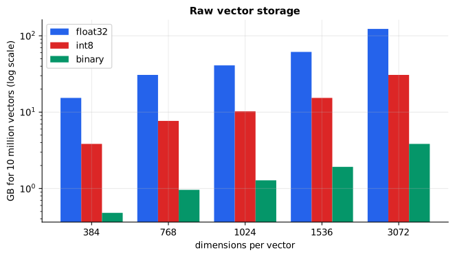
Ten million 3,072-dimension vectors take 123 GB as float32, 31 GB as int8 and under 4 GB as binary; smaller dimensions shrink each bar in proportion

Reading it: each group of bars is one common embedding size, from 384 to 3,072 dimensions. Within a group, the three bars are float32, int8 and binary storage for ten million vectors, on a log scale (each gridline is 10×). A 3,072-dimension float32 index needs over 120 GB of memory; the same vectors as bits fit in under 4 GB.

In code: storage_bytes computes n × d × b/8 exactly, and hnsw_link_bytes adds the 2·M neighbour ids an HNSW graph keeps per vector.

Why it matters: fast vector indexes like HNSW want every vector in RAM, so storage is the server bill. Being able to do this sum in your head tells you in seconds whether a design fits on one machine.

Matryoshka: important numbers first, then cut

Everyday picture: Russian nesting dolls: a small doll inside a bigger one inside a bigger one, each complete on its own. A Matryoshka embedding is trained so its first 64 numbers are a decent embedding, its first 256 a better one, and the full vector the best.

Tiny example: a vector (0.9, 0.4, 0.1, 0.05) where the numbers shrink in importance. Keep the first two, (0.9, 0.4), and rescale it to length 1 (divide by √(0.81 + 0.16) = 0.985): (0.914, 0.406). The dropped numbers were small, so the direction barely moves: its cosine with the full (normalized) vector is 0.994.

Level 3: the formula and its symbols

$$ v_{:m} = \frac{(v_1, \dots, v_m)}{\lVert (v_1, \dots, v_m) \rVert} $$

Symbols

Symbol	Meaning here	Shape
v	the full embedding	d numbers
m	how many leading numbers we keep	1 to d
v₁ … vₘ	the first m numbers	m numbers
‖·‖	length (norm)	one number
v₍:ₘ₎	the truncated, re-normalized vector	m numbers, length 1

In words: keep the first m numbers and rescale them to length 1.

On the example: m = 2: (0.9, 0.4) / 0.985 = (0.914, 0.406).

Level 3: in Python

In Python:

import math
v = [0.9, 0.4, 0.1, 0.05]
m = 2
# (v_1, ..., v_m)
prefix = v[:m]
# ‖(v_1, ..., v_m)‖
length = math.sqrt(sum(v_i ** 2 for v_i in prefix))
round(length, 3)  # → 0.985
# rescale to length 1
v_m = [v_i / length for v_i in prefix]
[round(v_i, 3) for v_i in v_m]  # → [0.914, 0.406]
full = math.sqrt(sum(v_i ** 2 for v_i in v))
# cosine with the full, normalized vector
round(sum(a * b / full for a, b in zip(v_m, v)), 3)  # → 0.994

This only works if the important numbers really come first. A real Matryoshka model is trained that way: the same contrastive loss (primer.ml.embeddings.contrastive) is applied to several prefixes at once (the first 64, 128, 256, … numbers), so each prefix must work on its own. Here we imitate it by rotating vectors onto their principal directions (the directions along which the collection varies most, found with the SVD; see primer.notation), which puts the most informative number first.

flowchart LR
  T[Text] --> E[Encoder] --> V["full vector (d numbers)"]
  V --> P64["first 64"] --> L64[loss]
  V --> P256["first 256"] --> L256[loss]
  V --> PD["all d"] --> LD[loss]
  L64 & L256 & LD --> S["sum: every prefix<br/>must work on its own"]

Reading it: one text, one encoder, one vector, scored several times. Each prefix of the vector is judged by the usual contrastive loss, and the model is trained on the sum. That's the whole trick: nothing about the model changes, only how its output is graded.

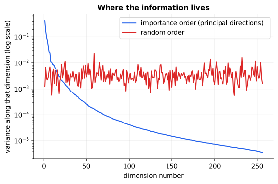
In importance order variance drops steeply, the first 16 of 256 dimensions holding 96% of it; in random order it stays in a narrow band with no standouts

Reading it: the horizontal axis is the dimension number and the vertical axis is how much the collection varies along it (its variance: the average squared distance from the mean, on a log scale). In importance order, the first few dimensions carry most of the variation and it falls steadily after that, so cutting from the end loses little. In a random order every dimension carries a similar share, so cutting any of them costs the same.

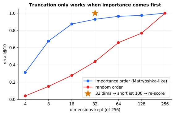
Keeping 32 of 256 dimensions finds 93% of true top-10 neighbours in importance order but 44% in random order; re-ranking a 100 shortlist finds all

Reading it: the horizontal axis is how many leading dimensions we keep (of 256); the vertical axis is recall@10, the share of each query's true top-10 neighbours we still find. In importance order, 32 dimensions (one eighth) still find about 93% of the neighbours; in random order they find about 44%. The star is the two-stage design: search with the first 32 numbers to shortlist 100 candidates, then re-rank those 100 with the full vectors. It finds all of them.

In code: matryoshka_order rotates vectors onto their principal directions, most informative first, and random_order is the control. search_truncated searches with the first m numbers only; search_truncated_then_rescore shortlists that way, then re-ranks the shortlist with the full vectors.

Measuring what compression costs: recall@k

Level 3: the formula and its symbols

$$ \text{recall@}k = \frac{\lvert \text{found}_k \cap \text{true}_k \rvert}{k} $$

Symbols

Symbol	Meaning here	Example
k	how many results we look at	10 in this lesson; 3 in the example
foundₖ	the k results the compressed search returned	(3, 4, 1)
trueₖ	the k results an exact, full-precision search returns	(1, 2, 3)
∩	"items in both"	{1, 3}
\|·\|	count the items	2

In words: the share of the true top-k that the compressed search also found.

On an example: true (1, 2, 3), found (3, 4, 1): two of the three appear, so recall@3 = 2/3 ≈ 0.67.

Level 3: in Python

In Python:

true_k = {1, 2, 3}
found_k = {3, 4, 1}
k = 3
# ∩: the items in both
found_k & true_k  # → {1, 3}
# |found ∩ true| / k
round(len(found_k & true_k) / k, 2)  # → 0.67

In code: recall_at_k averages this share over every query. top_k runs the exact full-precision search that supplies trueₖ, and make_corpus builds the documents, queries and true neighbours every experiment here uses.

Scalar quantization: 256 levels per number

Everyday picture: rounding prices to the nearest dollar. Here, every number is rounded to one of 256 marks on a ruler that runs from the smallest to the largest value seen in that dimension. 256 marks fit in one byte (int8), a quarter of a float's 4 bytes.

Tiny example: a dimension whose values run from lo = −1 to hi = 1. The 256 marks are 2/255 = 0.00784 apart. The value 0 sits at (0 − (−1)) / 2 × 255 = 127.5 marks, rounds to mark 128, and decodes back to −1 + 128/255 × 2 = 0.00392. It's off by 0.00392, half a mark, the worst case.

Level 3: the formula and its symbols

$$ \text{code} = \operatorname{round}!\left(\frac{x - lo}{hi - lo} \times 255\right), \qquad \hat{x} = lo + \frac{\text{code}}{255}\,(hi - lo) $$

Symbols

Symbol	Meaning here	Range
x	one number in a vector	between lo and hi (clipped if outside)
lo, hi	smallest and largest value of this dimension across the documents	calibrated once
(x − lo)/(hi − lo)	where x sits between lo and hi, as a fraction	0 to 1
× 255	stretch to the 256 marks 0 … 255	0 to 255
round	nearest whole number
code	the stored byte	0 to 255
x̂ (x-hat)	the value decoded back	within half a mark of x

In words: find where x sits between the dimension's minimum and maximum, turn that into one of 256 whole-number marks, and store the mark; to decode, walk back from the mark to the value.

On the example: x = 0, lo = −1, hi = 1: code = round(0.5 × 255) = round(127.5) = 128; x̂ = −1 + (128/255)·2 = 0.00392.

Level 3: in Python

In Python:

x, lo, hi = 0, -1, 1
# round(127.5): ties go to the even mark
code = round((x - lo) / (hi - lo) * 255)
code  # → 128
# decode: walk back from the mark
x_hat = lo + code / 255 * (hi - lo)
round(x_hat, 5)  # → 0.00392

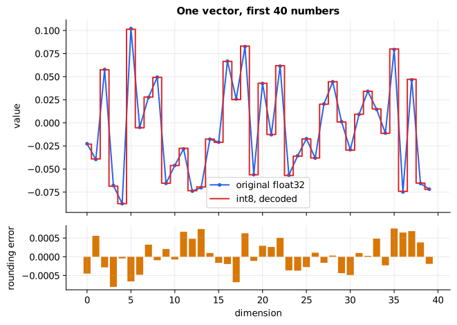
The decoded int8 steps track the first 40 numbers of the vector almost exactly; the rounding error never exceeds half of one step

Reading it: the line shows the first 40 numbers of one real vector from this lesson's corpus; the steps show the same numbers after rounding to 256 levels and decoding. The two are almost indistinguishable: the rounding error (the bottom panel) never exceeds half a mark. That's why int8 search here still finds about 98% of the true neighbours.

In code: scalar_quantize_int8 turns each number into its code, dequantize_int8 walks back to x̂, and search_int8 calibrates lo and hi on the documents and searches the decoded vectors.

Binary quantization: one bit per number

Everyday picture: a yes/no questionnaire. For each number, record only "positive: yes or no". Two texts are compared by counting how many answers differ, the Hamming distance.

Tiny example: the eight values (0.3, −0.2, 0.0, 5, −1, 2, −3, 0.1) become the bits 1 0 0 1 0 1 0 1, packed into one byte: 0b10010101 = 149. Compare with 0b00010100: they differ in the first and last positions, so the Hamming distance is 2.

Level 3: the formula and its symbols

$$ \text{bit}_i = [\,x_i > 0\,], \qquad \text{hamming}(a, b) = \sum_{i=1}^{d} [\,a_i \ne b_i\,] $$

Symbols

Symbol	Meaning here	Range
xᵢ	the i-th number of the vector	any real number
[ condition ]	1 if the condition is true, 0 if not	0 or 1
bitᵢ	the stored bit for position i	0 or 1
a, b	two bit codes being compared	d bits each
aᵢ ≠ bᵢ	the two codes disagree at position i
Σ	add up over all d positions
hamming(a, b)	number of positions that disagree	0 to d

In words: keep one bit per number that says whether it was positive, and measure distance as the number of positions where two codes disagree.

On the example: 149 = 10010101 vs 20 = 00010100: positions 1 and 8 differ, so the distance is 2. Computers do this with one XOR (mark the differing bits) and one popcount (count them), which is why binary search is extremely fast.

Level 3: in Python

In Python:

x = [0.3, -0.2, 0.0, 5, -1, 2, -3, 0.1]
# bit_i = [x_i > 0]
a = [int(x_i > 0) for x_i in x]
a  # → [1, 0, 0, 1, 0, 1, 0, 1]
# packed into one byte
int("".join(map(str, a)), 2)  # → 149
# 0b00010100 = 20
b = [0, 0, 0, 1, 0, 1, 0, 0]
# hamming(a, b) = Σ [a_i ≠ b_i]
sum(a_i != b_i for a_i, b_i in zip(a, b))  # → 2
# the computer's way: XOR, then count the 1s
bin(149 ^ 20).count("1")  # → 2

flowchart LR
  Q[Query] --> B["Stage 1: bits + Hamming<br/>scan all 5,000 docs<br/>(32× smaller, very fast)"]
  B --> S[Shortlist of 100]
  S --> F["Stage 2: full float vectors<br/>exact dot product on 100 only"]
  F --> T[Top 10]
  STORE[("bits for every doc (RAM)<br/>floats for every doc (disk or RAM)")] --> B
  STORE --> F

Reading it: the cheap representation is used where the work is big (every document), and the expensive one where the work is small (100 candidates). The bits live in fast memory; the full vectors can live somewhere slower because only a hundred are read per query.

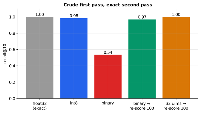
Recall@10: int8 keeps 0.98 and binary alone only 0.54, but binary re-scored over 100 candidates recovers 0.97 and a 32-dimension shortlist reaches 1.00

Reading it: each bar is one way of storing the documents, measured by recall@10 against exact float32 search. int8 alone keeps about 98%. Binary alone keeps only about half: signs lose a lot. But binary as a shortlist, re-scored with full vectors, climbs back to about 97%, and 32-dimension Matryoshka shortlists to 100%. Crude-then-exact is the pattern to remember.

In code: binary_quantize keeps each number's sign and packs 8 bits per byte, and hamming_distances counts differing bits with XOR and a popcount table. search_binary ranks by bits alone; search_binary_then_rescore re-ranks the bit-based shortlist with the full float vectors.

Why it matters: these knobs move real money. Many vector databases ship int8 and binary quantization with re-scoring built in, and embedding providers increasingly ship Matryoshka-trained models so you can pick your dimension. The cost is always measured the same way: recall@k on your own queries.

In 20 seconds

Raw storage is n × d × bytes per number: 10M × 1,536 float32 ≈ 61 GB, before index overhead.
Matryoshka models put the important information in the leading numbers, so you can truncate and re-normalize.
int8 stores 256 levels per number (4× smaller, little loss); binary keeps signs only (32× smaller, big loss alone).
Shortlist with the crude form, re-score with full vectors: most of the quality at a fraction of the memory.
Always measure the cost as recall@k against exact search.

Self-test questions

Q: How much memory do ten million 1,536-dimension float32 vectors need? 10,000,000 × 1,536 × 4 bytes = 61.4 GB of raw vectors, plus index overhead (e.g. ~1.3 GB of HNSW links at M = 16).

Q: What makes Matryoshka embeddings truncatable, and how do you use that? They're trained with the loss applied to several prefixes at once, so the first m numbers form a good embedding by themselves. Search with short vectors for speed and memory, then re-score the top candidates with the full vectors.

Q: Scalar vs. binary quantization: what do you give up? int8 rounds each number to 256 levels, 4× smaller with a small recall loss. Binary keeps only signs, 32× smaller, but recall drops a lot on its own; it works as a first-stage shortlist followed by full-precision re-scoring.

Q: Why not just use as many dimensions as possible? Gains flatten out while storage, memory and search time grow linearly. A smaller model trained for your domain often beats a bigger generic one, so benchmark on your own queries.

The papers behind this lesson

Kusupati et al., Matryoshka Representation Learning (2022): https://arxiv.org/abs/2205.13147. Trained embeddings whose every prefix is a usable embedding, by summing the loss over nested prefix lengths. annotated companion

Hugging Face, Embedding Quantization (binary and int8 with re-scoring): https://huggingface.co/blog/embedding-quantization
Hugging Face, Introduction to Matryoshka Embedding Models: https://huggingface.co/blog/matryoshka
Faiss wiki, Guidelines to choose an index: https://github.com/facebookresearch/faiss/wiki/Guidelines-to-choose-an-index

View Sourceon GitHub

  1r"""
  2# Compression: smaller vectors, same neighbours
  3
  4Run: `python -m primer.ml.embeddings.compression`
  5
  6New to vectors, dimensions or Σ? `primer.notation` builds them from zero.
  7
  8## Level 1: The practitioner's guide
  9
 10**In one sentence.** Embedding compression stores each vector in fewer
 11numbers, or rougher ones, so that an index of millions fits in memory and
 12searches faster, while still returning the same neighbours as the full
 13vectors would.
 14
 15**When you need it.** The moment a vector index stops fitting on the machine
 16you meant to run it on, or its bill stops fitting the budget. Do the sum
 17before you pick either: vectors × dimensions × 4 bytes. Ten million
 181,536-dimension vectors are 61 GB as 32-bit floats, before the index adds
 19its own links (about 1.3 GB for an HNSW graph at 16 links per node); at
 203,072 dimensions it is 123 GB. Fast indexes keep every vector in RAM, so
 21that number is the server. The tell is a search service whose memory line is
 22the vectors themselves, or an embedding upgrade to a longer model that
 23doubled the hosting cost. You don't need any of this while the sum is small
 24(a hundred thousand 1,536-dimension vectors are 0.6 GB of floats), and you
 25never need it at the price of neighbours you can't measure: the cost of
 26every option here is recall@k against exact search on your own queries.
 27
 28**Your options.** From the least saving to the most, each measured in this
 29lesson on 5,000 documents of 256 dimensions:
 30
 31| Option | What it does | What it guarantees | What it costs | Where it lives |
 32|---|---|---|---|---|
 33| Full float32 | Stores every number as is | Exact: recall 1.00 by definition | 4 bytes per dimension; 61 GB for 10M × 1,536 | The default everywhere |
 34| Half precision | Stores each number in 2 bytes instead of 4 | Halves storage and keeps every dimension | 16-bit rounding, small but still to be measured | The column type (pgvector's halfvec) |
 35| Fewer dimensions (Matryoshka) | Keeps the first m numbers of a vector trained so the important ones come first, and re-normalizes | Any size you choose, with graceful loss: 32 of 256 dimensions keep 93% of the top-10 neighbours here; 98% of benchmark performance at 8% of the size in Hugging Face's tests | A model trained for it; a random model loses more than half its neighbours at the same cut | The embedding call (a dimensions parameter) or your write path |
 36| int8 scalar quantization | Rounds each number to one of 256 levels between the dimension's minimum and maximum | 4× smaller with little loss: recall 0.98 here, about 99% retained in Hugging Face's benchmarks | A calibration pass to find each dimension's range, and clipping for values outside it | The database's quantization setting |
 37| Binary with re-scoring | Keeps one bit per number (its sign), searches by counting differing bits, then re-ranks a shortlist with the full vectors | 32× smaller in the fast path: bits alone keep 0.54 of the neighbours here, re-scoring the top 100 brings back 0.97 | The full vectors kept somewhere slower for the re-score, and a second stage per query | Index settings with rescoring or oversampling on |
 38| Product quantization | Splits each vector into chunks and replaces every chunk with the id of its nearest learned centroid | Up to 64× (Qdrant's figure) when memory is everything | A training step for the codebooks and the largest quality loss; measure before trusting it | Faiss, Qdrant |
 39| Two stages combined | Shortlists with a short or binary form, re-ranks with full vectors | Most of the quality at a fraction of the memory: 32 dimensions to shortlist 100, full vectors to re-rank, recall 1.00 here | Full vectors on disk, two lookups per query | Your search code, or an index with rescoring built in |
 40
 41**How to choose.** Start from the sum, then from what your model supports.
 42
 43- It fits with headroom: change nothing. Every option below costs neighbours
 44  or complexity.
 45- Your model exposes a dimensions parameter (it was trained Matryoshka
 46  style): cut dimensions first. It is the cheapest knob and it shrinks
 47  compute per comparison as well as memory.
 48- Memory tight by a factor of a few: int8. It is the safe default; 4× for a
 49  loss you will struggle to see.
 50- Memory tight by an order of magnitude, or a corpus in the hundreds of
 51  millions: binary for the scan, floats on disk for the re-score, with the
 52  shortlist size tuned until recall@10 on your queries is back where you
 53  need it.
 54- Whatever you pick, measure recall@k against exact float search on a sample
 55  of your own queries before and after, and keep the number with the index
 56  configuration.
 57
 58**What it costs.** Memory follows the bytes: for 10 million 1,536-dimension
 59vectors, 61 GB as float32, 15 GB as int8, 1.9 GB as bits (this lesson's
 60sum). Hugging Face's benchmark prices it at 250 million 1,024-dimension
 61vectors on a cloud instance: about \$3,623 a month as float32, \$905 as int8,
 62\$113 as binary. Speed follows memory: binary search runs up to 45× faster
 63than float in that benchmark (a mean of 25×), int8 up to 4×. Quality is the
 64cost you pay in neighbours: here int8 loses 2% of the top-10, binary alone
 65loses 46% and gets 43 points back from re-scoring, and Matryoshka at one
 66eighth of the dimensions loses 7%. Effort is a calibration pass for int8,
 67a training step for product quantization, and a second query stage for any
 68two-stage design. Nothing here changes the model or its vectors' meaning:
 69compression is applied on the write path and can be undone by re-indexing.
 70
 71**What breaks.**
 72
 73- **Truncating a model not trained for it.** Cut a plain model's vector to
 74  32 of 256 dimensions and recall@10 drops to 0.44; the same cut on
 75  importance-ordered vectors keeps 0.93. Check the model card, or order the
 76  dimensions yourself as Level 2 does.
 77- **Forgetting to re-normalize.** A truncated vector is shorter than 1; the
 78  provider's parameter does this for you, a manual slice does not, and
 79  OpenAI's guide says so in as many words.
 80- **Binary as the final answer.** Signs alone keep half the neighbours. Bits
 81  are a shortlist, never the ranking.
 82- **A calibration range that drifted.** int8's levels span the minimum and
 83  maximum seen at calibration; documents added later that fall outside are
 84  clipped. Recalibrate when the corpus changes character.
 85- **Bits on bunched vectors.** Vectors that crowd into a narrow cone
 86  (`primer.ml.embeddings.similarity`) share most of their signs, so their
 87  bits carry little; Qdrant recommends binary for centred, high-dimensional
 88  distributions. Mean-centre first, or pick int8.
 89- **Measuring on someone else's queries.** A benchmark's recall is not
 90  yours. Sample your own queries and compare against exact search.
 91- **Counting only the vectors.** The graph's links, the full vectors kept for
 92  re-scoring and the working memory of a build all add to the bill.
 93
 94**In the wild.** OpenAI's text-embedding-3 models take a dimensions
 95parameter that shortens their 1,536 or 3,072 numbers; Cohere's embed-v4.0
 96offers 256 to 1,536 dimensions and returns float, int8, uint8, binary or
 97ubinary embeddings from one call; Nomic's nomic-embed-text-v1.5 is an open
 98Matryoshka model, and sentence-transformers trains one with MatryoshkaLoss
 99wrapped around any base loss. Qdrant ships scalar, binary and product
100quantization with rescoring and oversampling; pgvector has a halfvec column,
101a bit column and a binary_quantize function for its HNSW indexes; Faiss
102offers scalar quantizers, product quantization (PQ, OPQ) and RaBitQ at about
103d/8 + 8 bytes per vector. The idea comes from Kusupati et al. (2022),
104Matryoshka Representation Learning, which reported up to 14× smaller
105embeddings at the same ImageNet accuracy and up to 14× faster retrieval; the
106numbers above come from Hugging Face's embedding quantization and Matryoshka
107posts and from this lesson's own experiment.
108
109**Go deeper.** Level 2 does the byte arithmetic, builds Matryoshka ordering
110from a principal-direction rotation and measures recall as dimensions fall
111away, rounds a real vector to 256 levels and shows the error never exceeds
112half a step, packs signs into bytes and counts differing bits with one XOR,
113and runs the two-stage search that gets the neighbours back. If you only
114needed to choose, you are done.
115
116## Level 2: How it works, from scratch
117
118An embedding describes a text with a long list of numbers, like describing
119a person with hundreds of adjectives. More adjectives let you tell very
120similar people apart, but every adjective takes shelf space, and a search
121system has to keep millions of these descriptions in fast memory.
122
123This lesson is about making the descriptions smaller without mixing people
124up. There are three tricks, each with an everyday twin:
125
126- **Keep fewer numbers** (Matryoshka truncation): a well-written news story
127  puts the headline first and the details later, so you can cut from the
128  bottom and still know what happened.
129- **Store each number more roughly** (scalar quantization): round every
130  price to the nearest dollar. Totals barely change, and the list gets much
131  shorter to write down.
132- **Keep only a yes/no per number** (binary quantization): instead of
133  "4.7 out of 10", just record "above average: yes". Crude, but amazingly
134  good for a first sort.
135
136And one trick that rescues the crude ones: **shortlist, then check**. Skim a
137pile of CVs fast to pick 100, then read those 100 carefully.
138
139## A tiny worked example: counting bytes
140
141A **dimension** is one number in the vector. A 32-bit float (the usual
142format) takes 4 bytes. So one 1,536-dimension vector takes 1,536 × 4 = 6,144
143bytes, and ten million of them take:
144
145$$
146\text{bytes} = n \times d \times \frac{b}{8}
147$$
148
149**Symbols**
150
151| Symbol | Meaning here | Example value |
152|---|---|---|
153| n | number of vectors | 10,000,000 |
154| d | dimensions per vector | 1,536 |
155| b | bits per number | 32 (float32), 8 (int8), 1 (binary) |
156| b / 8 | bytes per number (8 bits in a byte) | 4, 1, or 1/8 |
157
158**In words:** storage is the number of vectors, times the numbers in each,
159times the bytes per number.
160
161**On the example:** 10,000,000 × 1,536 × 32/8 = **61,440,000,000 bytes ≈ 61 GB**.
162As int8 it's **15.4 GB**; as bits, **1.9 GB**.
163
164**In Python:**
165
166```python
167n, d = 10_000_000, 1536
168# float32, int8, binary
169for b in (32, 8, 1):
170    # bytes = n × d × b/8
171    size = n * d * b // 8
172    print(b, size, round(size / 1e9, 1), "GB")  # → 32 61440000000 61.4 GB 8 15360000000 15.4 GB 1 1920000000 1.9 GB
173# HNSW: 2·M ids of 4 bytes each, M = 16, in GB
174n * 2 * 16 * 4 / 1e9  # → 1.28
175```
176
177The index adds its own overhead. An HNSW graph (`primer.ml.embeddings.ann`)
178stores about 2·M neighbour ids per vector at 4 bytes each: with M = 16 that's
17910M × 32 × 4 = **1.28 GB** more.
180
181![Ten million 3,072-dimension vectors take 123 GB as float32, 31 GB as int8 and under 4 GB as binary; smaller dimensions shrink each bar in proportion](figures/primer.ml.embeddings.compression.storage.svg)
182
183**Reading it:** each group of bars is one common embedding size, from 384 to
1843,072 dimensions. Within a group, the three bars are float32, int8 and
185binary storage for ten million vectors, on a log scale (each gridline is 10×).
186A 3,072-dimension float32 index needs over 120 GB of memory; the same
187vectors as bits fit in under 4 GB.
188
189**In code:** `storage_bytes` computes n × d × b/8 exactly, and
190`hnsw_link_bytes` adds the 2·M neighbour ids an HNSW graph keeps per vector.
191
192**Why it matters:** fast vector indexes like HNSW want every vector in RAM,
193so storage *is* the server bill. Being able to do this sum in your head
194tells you in seconds whether a design fits on one machine.
195
196## Matryoshka: important numbers first, then cut
197
198**Everyday picture:** Russian nesting dolls: a small doll inside a bigger one
199inside a bigger one, each complete on its own. A **Matryoshka embedding** is
200trained so its first 64 numbers are a decent embedding, its first 256 a
201better one, and the full vector the best.
202
203**Tiny example:** a vector (0.9, 0.4, 0.1, 0.05) where the numbers shrink in
204importance. Keep the first two, (0.9, 0.4), and rescale it to length 1
205(divide by √(0.81 + 0.16) = 0.985): (0.914, 0.406). The dropped numbers were
206small, so the direction barely moves: its cosine with the full (normalized)
207vector is 0.994.
208
209$$
210v_{:m} = \frac{(v_1, \dots, v_m)}{\lVert (v_1, \dots, v_m) \rVert}
211$$
212
213**Symbols**
214
215| Symbol | Meaning here | Shape |
216|---|---|---|
217| v | the full embedding | d numbers |
218| m | how many leading numbers we keep | 1 to d |
219| v₁ … vₘ | the first m numbers | m numbers |
220| ‖·‖ | length (norm) | one number |
221| v₍:ₘ₎ | the truncated, re-normalized vector | m numbers, length 1 |
222
223**In words:** keep the first m numbers and rescale them to length 1.
224
225**On the example:** m = 2: (0.9, 0.4) / 0.985 = (0.914, 0.406).
226
227**In Python:**
228
229```python
230import math
231v = [0.9, 0.4, 0.1, 0.05]
232m = 2
233# (v_1, ..., v_m)
234prefix = v[:m]
235# ‖(v_1, ..., v_m)‖
236length = math.sqrt(sum(v_i ** 2 for v_i in prefix))
237round(length, 3)  # → 0.985
238# rescale to length 1
239v_m = [v_i / length for v_i in prefix]
240[round(v_i, 3) for v_i in v_m]  # → [0.914, 0.406]
241full = math.sqrt(sum(v_i ** 2 for v_i in v))
242# cosine with the full, normalized vector
243round(sum(a * b / full for a, b in zip(v_m, v)), 3)  # → 0.994
244```
245
246This only works if the important numbers really come first. A real
247Matryoshka model is *trained* that way: the same contrastive loss
248(`primer.ml.embeddings.contrastive`) is applied to several prefixes at once
249(the first 64, 128, 256, … numbers), so each prefix must work on its own.
250Here we imitate it by rotating vectors onto their **principal directions**
251(the directions along which the collection varies most, found with the SVD;
252see `primer.notation`), which puts the most informative number first.
253
254```mermaid
255flowchart LR
256  T[Text] --> E[Encoder] --> V["full vector (d numbers)"]
257  V --> P64["first 64"] --> L64[loss]
258  V --> P256["first 256"] --> L256[loss]
259  V --> PD["all d"] --> LD[loss]
260  L64 & L256 & LD --> S["sum: every prefix<br/>must work on its own"]
261```
262
263**Reading it:** one text, one encoder, one vector, scored several times. Each
264prefix of the vector is judged by the usual contrastive loss, and the model
265is trained on the sum. That's the whole trick: nothing about the model
266changes, only how its output is graded.
267
268![In importance order variance drops steeply, the first 16 of 256 dimensions holding 96% of it; in random order it stays in a narrow band with no standouts](figures/primer.ml.embeddings.compression.spectrum.svg)
269
270**Reading it:** the horizontal axis is the dimension number and the vertical
271axis is how much the collection varies along it (its **variance**: the
272average squared distance from the mean, on a log scale). In importance
273order, the first few dimensions carry most of the variation and it falls
274steadily after that, so cutting from the end loses little. In a random
275order every dimension carries a similar share, so cutting any of them costs
276the same.
277
278![Keeping 32 of 256 dimensions finds 93% of true top-10 neighbours in importance order but 44% in random order; re-ranking a 100 shortlist finds all](figures/primer.ml.embeddings.compression.matryoshka.svg)
279
280**Reading it:** the horizontal axis is how many leading dimensions we keep
281(of 256); the vertical axis is **recall@10**, the share of each query's true
282top-10 neighbours we still find. In importance order, 32 dimensions (one
283eighth) still find about 93% of the neighbours; in random order they find
284about 44%. The star is the two-stage design: search with the first 32
285numbers to shortlist 100 candidates, then re-rank those 100 with the full
286vectors. It finds all of them.
287
288**In code:** `matryoshka_order` rotates vectors onto their principal
289directions, most informative first, and `random_order` is the control.
290`search_truncated` searches with the first m numbers only;
291`search_truncated_then_rescore` shortlists that way, then re-ranks the
292shortlist with the full vectors.
293
294## Measuring what compression costs: recall@k
295
296$$
297\text{recall@}k = \frac{\lvert \text{found}_k \cap \text{true}_k \rvert}{k}
298$$
299
300**Symbols**
301
302| Symbol | Meaning here | Example |
303|---|---|---|
304| k | how many results we look at | 10 in this lesson; 3 in the example |
305| foundₖ | the k results the compressed search returned | (3, 4, 1) |
306| trueₖ | the k results an exact, full-precision search returns | (1, 2, 3) |
307| ∩ | "items in both" | {1, 3} |
308| \|·\| | count the items | 2 |
309
310**In words:** the share of the true top-k that the compressed search also
311found.
312
313**On an example:** true (1, 2, 3), found (3, 4, 1): two of the three appear,
314so recall@3 = 2/3 ≈ 0.67.
315
316**In Python:**
317
318```python
319true_k = {1, 2, 3}
320found_k = {3, 4, 1}
321k = 3
322# ∩: the items in both
323found_k & true_k  # → {1, 3}
324# |found ∩ true| / k
325round(len(found_k & true_k) / k, 2)  # → 0.67
326```
327
328**In code:** `recall_at_k` averages this share over every query. `top_k`
329runs the exact full-precision search that supplies trueₖ, and `make_corpus`
330builds the documents, queries and true neighbours every experiment here
331uses.
332
333## Scalar quantization: 256 levels per number
334
335**Everyday picture:** rounding prices to the nearest dollar. Here, every
336number is rounded to one of 256 marks on a ruler that runs from the smallest
337to the largest value seen in that dimension. 256 marks fit in one byte
338(**int8**), a quarter of a float's 4 bytes.
339
340**Tiny example:** a dimension whose values run from lo = −1 to hi = 1. The 256
341marks are 2/255 = 0.00784 apart. The value 0 sits at (0 − (−1)) / 2 × 255 = 127.5
342marks, rounds to mark **128**, and decodes back to −1 + 128/255 × 2 = **0.00392**.
343It's off by 0.00392, half a mark, the worst case.
344
345$$
346\text{code} = \operatorname{round}\!\left(\frac{x - lo}{hi - lo} \times 255\right),
347\qquad \hat{x} = lo + \frac{\text{code}}{255}\,(hi - lo)
348$$
349
350**Symbols**
351
352| Symbol | Meaning here | Range |
353|---|---|---|
354| x | one number in a vector | between lo and hi (clipped if outside) |
355| lo, hi | smallest and largest value of this dimension across the documents | calibrated once |
356| (x − lo)/(hi − lo) | where x sits between lo and hi, as a fraction | 0 to 1 |
357| × 255 | stretch to the 256 marks 0 … 255 | 0 to 255 |
358| round | nearest whole number | |
359| code | the stored byte | 0 to 255 |
360| x̂ (x-hat) | the value decoded back | within half a mark of x |
361
362**In words:** find where x sits between the dimension's minimum and maximum,
363turn that into one of 256 whole-number marks, and store the mark; to decode,
364walk back from the mark to the value.
365
366**On the example:** x = 0, lo = −1, hi = 1: code = round(0.5 × 255) = round(127.5) = 128;
367x̂ = −1 + (128/255)·2 = 0.00392.
368
369**In Python:**
370
371```python
372x, lo, hi = 0, -1, 1
373# round(127.5): ties go to the even mark
374code = round((x - lo) / (hi - lo) * 255)
375code  # → 128
376# decode: walk back from the mark
377x_hat = lo + code / 255 * (hi - lo)
378round(x_hat, 5)  # → 0.00392
379```
380
381![The decoded int8 steps track the first 40 numbers of the vector almost exactly; the rounding error never exceeds half of one step](figures/primer.ml.embeddings.compression.int8.svg)
382
383**Reading it:** the line shows the first 40 numbers of one real vector from
384this lesson's corpus; the steps show the same numbers after rounding to
385256 levels and decoding. The two are almost indistinguishable: the rounding
386error (the bottom panel) never exceeds half a mark. That's why int8 search
387here still finds about 98% of the true neighbours.
388
389**In code:** `scalar_quantize_int8` turns each number into its code,
390`dequantize_int8` walks back to x̂, and `search_int8` calibrates lo and hi
391on the documents and searches the decoded vectors.
392
393## Binary quantization: one bit per number
394
395**Everyday picture:** a yes/no questionnaire. For each number, record only
396"positive: yes or no". Two texts are compared by counting how many answers
397differ, the **Hamming distance**.
398
399**Tiny example:** the eight values (0.3, −0.2, 0.0, 5, −1, 2, −3, 0.1) become the
400bits 1 0 0 1 0 1 0 1, packed into one byte: 0b10010101 = **149**. Compare with
4010b00010100: they differ in the first and last positions, so the Hamming
402distance is **2**.
403
404$$
405\text{bit}_i = [\,x_i > 0\,], \qquad
406\text{hamming}(a, b) = \sum_{i=1}^{d} [\,a_i \ne b_i\,]
407$$
408
409**Symbols**
410
411| Symbol | Meaning here | Range |
412|---|---|---|
413| xᵢ | the i-th number of the vector | any real number |
414| [ condition ] | 1 if the condition is true, 0 if not | 0 or 1 |
415| bitᵢ | the stored bit for position i | 0 or 1 |
416| a, b | two bit codes being compared | d bits each |
417| aᵢ ≠ bᵢ | the two codes disagree at position i | |
418| Σ | add up over all d positions | |
419| hamming(a, b) | number of positions that disagree | 0 to d |
420
421**In words:** keep one bit per number that says whether it was positive, and
422measure distance as the number of positions where two codes disagree.
423
424**On the example:** 149 = 10010101 vs 20 = 00010100: positions 1 and 8 differ,
425so the distance is 2. Computers do this with one XOR (mark the differing
426bits) and one popcount (count them), which is why binary search is extremely
427fast.
428
429**In Python:**
430
431```python
432x = [0.3, -0.2, 0.0, 5, -1, 2, -3, 0.1]
433# bit_i = [x_i > 0]
434a = [int(x_i > 0) for x_i in x]
435a  # → [1, 0, 0, 1, 0, 1, 0, 1]
436# packed into one byte
437int("".join(map(str, a)), 2)  # → 149
438# 0b00010100 = 20
439b = [0, 0, 0, 1, 0, 1, 0, 0]
440# hamming(a, b) = Σ [a_i ≠ b_i]
441sum(a_i != b_i for a_i, b_i in zip(a, b))  # → 2
442# the computer's way: XOR, then count the 1s
443bin(149 ^ 20).count("1")  # → 2
444```
445
446```mermaid
447flowchart LR
448  Q[Query] --> B["Stage 1: bits + Hamming<br/>scan all 5,000 docs<br/>(32× smaller, very fast)"]
449  B --> S[Shortlist of 100]
450  S --> F["Stage 2: full float vectors<br/>exact dot product on 100 only"]
451  F --> T[Top 10]
452  STORE[("bits for every doc (RAM)<br/>floats for every doc (disk or RAM)")] --> B
453  STORE --> F
454```
455
456**Reading it:** the cheap representation is used where the work is big (every
457document), and the expensive one where the work is small (100 candidates).
458The bits live in fast memory; the full vectors can live somewhere slower
459because only a hundred are read per query.
460
461![Recall@10: int8 keeps 0.98 and binary alone only 0.54, but binary re-scored over 100 candidates recovers 0.97 and a 32-dimension shortlist reaches 1.00](figures/primer.ml.embeddings.compression.quantization.svg)
462
463**Reading it:** each bar is one way of storing the documents, measured by
464recall@10 against exact float32 search. int8 alone keeps about 98%. Binary
465alone keeps only about half: signs lose a lot. But binary as a *shortlist*,
466re-scored with full vectors, climbs back to about 97%, and 32-dimension
467Matryoshka shortlists to 100%. Crude-then-exact is the pattern to remember.
468
469**In code:** `binary_quantize` keeps each number's sign and packs 8 bits per
470byte, and `hamming_distances` counts differing bits with XOR and a popcount
471table. `search_binary` ranks by bits alone; `search_binary_then_rescore`
472re-ranks the bit-based shortlist with the full float vectors.
473
474**Why it matters:** these knobs move real money. Many vector databases ship
475int8 and binary quantization with re-scoring built in, and embedding
476providers increasingly ship Matryoshka-trained models so you can pick your
477dimension. The cost is always measured the same way: recall@k on your own
478queries.
479
480## In 20 seconds
481- Raw storage is n × d × bytes per number: 10M × 1,536 float32 ≈ 61 GB, before
482  index overhead.
483- Matryoshka models put the important information in the leading numbers,
484  so you can truncate and re-normalize.
485- int8 stores 256 levels per number (4× smaller, little loss); binary keeps
486  signs only (32× smaller, big loss alone).
487- Shortlist with the crude form, re-score with full vectors: most of the
488  quality at a fraction of the memory.
489- Always measure the cost as recall@k against exact search.
490
491## Self-test questions
492
493**Q: How much memory do ten million 1,536-dimension float32 vectors need?**
49410,000,000 × 1,536 × 4 bytes = 61.4 GB of raw vectors, plus index overhead
495(e.g. ~1.3 GB of HNSW links at M = 16).
496
497**Q: What makes Matryoshka embeddings truncatable, and how do you use that?**
498They're trained with the loss applied to several prefixes at once, so the
499first m numbers form a good embedding by themselves. Search with short
500vectors for speed and memory, then re-score the top candidates with the
501full vectors.
502
503**Q: Scalar vs. binary quantization: what do you give up?**
504int8 rounds each number to 256 levels, 4× smaller with a small recall loss.
505Binary keeps only signs, 32× smaller, but recall drops a lot on its own; it
506works as a first-stage shortlist followed by full-precision re-scoring.
507
508**Q: Why not just use as many dimensions as possible?**
509Gains flatten out while storage, memory and search time grow linearly.
510A smaller model trained for your domain often beats a bigger generic one,
511so benchmark on your own queries.
512
513## The papers behind this lesson
514
515- **Kusupati et al., *Matryoshka Representation Learning* (2022)**: https://arxiv.org/abs/2205.13147.
516  Trained embeddings whose every prefix is a usable embedding, by summing the loss over nested prefix lengths. [annotated companion](../../../papers/matryoshka.html)
517
518## Further reading
519- Hugging Face, *Embedding Quantization* (binary and int8 with re-scoring): https://huggingface.co/blog/embedding-quantization
520- Hugging Face, *Introduction to Matryoshka Embedding Models*: https://huggingface.co/blog/matryoshka
521- Faiss wiki, *Guidelines to choose an index*: https://github.com/facebookresearch/faiss/wiki/Guidelines-to-choose-an-index
522"""
523
524from __future__ import annotations
525
526import numpy as np
527
528from primer._show import banner, say, table, takeaway
529
530# ---------------------------------------------------------------------------
531# 1. Storage math
532# ---------------------------------------------------------------------------
533
534
535def storage_bytes(n_vectors: int, dim: int, bits_per_value: int = 32) -> int:
536    """Raw bytes to store n vectors of `dim` numbers at `bits_per_value` each.
537
538    float32 = 32 bits, int8 = 8 bits, binary = 1 bit. Integer arithmetic so
539    the answer is exact.
540    """
541    return n_vectors * dim * bits_per_value // 8
542
543
544def hnsw_link_bytes(n_vectors: int, M: int = 16, bytes_per_link: int = 4) -> int:
545    """Bytes for the bottom layer of an HNSW graph: 2·M neighbour ids per vector.
546
547    Upper layers hold only a small fraction of the vectors, so they add a few
548    percent more; this is the part that scales with every vector.
549    (See `primer.ml.embeddings.ann` for how HNSW works.)
550    """
551    return n_vectors * 2 * M * bytes_per_link
552
553
554# ---------------------------------------------------------------------------
555# 2. A test corpus with realistic structure, and the recall metric
556# ---------------------------------------------------------------------------
557
558
559def _unit(X: np.ndarray) -> np.ndarray:
560    return X / np.linalg.norm(X, axis=-1, keepdims=True)
561
562
563def make_corpus(n_docs: int = 5000, n_queries: int = 100, dim: int = 256, k: int = 10, seed: int = 0):
564    """Docs, queries and each query's true top-k neighbours (by exact cosine).
565
566    Real embeddings aren't uniform noise: a few directions carry most of the
567    variation. We build that in: 50 topic clusters, a spread along direction
568    i that shrinks like 1/i, and then a random rotation so the raw coordinates
569    show no order (like a real model's output). Queries are noisy copies of
570    random docs.
571    """
572    rng = np.random.default_rng(seed)
573    scales = 1 / np.arange(1, dim + 1)  # spread along direction i ∝ 1/i: a few directions dominate
574    centers = rng.standard_normal((50, dim)) * scales
575    docs = centers[rng.integers(50, size=n_docs)] + 0.6 * rng.standard_normal((n_docs, dim)) * scales
576    R, _ = np.linalg.qr(rng.standard_normal((dim, dim)))  # random orthogonal matrix
577    docs = _unit(docs @ R)
578    queries = _unit(docs[rng.integers(n_docs, size=n_queries)] + 0.03 * rng.standard_normal((n_queries, dim)))
579    truth = top_k(docs, queries, k)
580    return docs, queries, truth
581
582
583def top_k(docs: np.ndarray, queries: np.ndarray, k: int) -> np.ndarray:
584    """Indices of the k highest dot products per query, best first. Shape (n_queries, k)."""
585    S = queries @ docs.T
586    idx = np.argpartition(-S, k, axis=1)[:, :k]  # the k best, unordered (cheaper than a full sort)
587    order = np.argsort(-np.take_along_axis(S, idx, axis=1), axis=1)
588    return np.take_along_axis(idx, order, axis=1)
589
590
591def recall_at_k(found: np.ndarray, truth: np.ndarray) -> float:
592    """Average share of each query's true neighbours that appear in what was found."""
593    return float(np.mean([len(set(f) & set(t)) / len(t) for f, t in zip(found, truth)]))
594
595
596# ---------------------------------------------------------------------------
597# 3. Matryoshka: put the important directions first, then truncate
598# ---------------------------------------------------------------------------
599
600
601def matryoshka_order(docs: np.ndarray, X: np.ndarray | None = None) -> np.ndarray:
602    """Rotate so dimension 1 carries the most variation, dimension 2 the next, and so on.
603
604    A real Matryoshka model is *trained* so every prefix is a good embedding.
605    Rotating onto the principal directions (the SVD of the doc matrix, see
606    `primer.notation`) is the closest do-it-yourself imitation, and it
607    shows the same effect. A rotation changes no dot product, so full-length
608    search is untouched; only truncation behaves differently.
609    """
610    _, _, Vt = np.linalg.svd(docs, full_matrices=False)
611    return (docs if X is None else X) @ Vt.T
612
613
614def random_order(docs: np.ndarray, X: np.ndarray | None = None, seed: int = 1) -> np.ndarray:
615    """A random rotation: every dimension carries a similar share of the information."""
616    R, _ = np.linalg.qr(np.random.default_rng(seed).standard_normal((docs.shape[1], docs.shape[1])))
617    return (docs if X is None else X) @ R
618
619
620def search_truncated(docs: np.ndarray, queries: np.ndarray, truth: np.ndarray, dims: int) -> float:
621    """recall@k using only the first `dims` numbers of every vector (re-normalized)."""
622    return recall_at_k(top_k(_unit(docs[:, :dims]), _unit(queries[:, :dims]), truth.shape[1]), truth)
623
624
625def search_truncated_then_rescore(docs, queries, truth, dims: int, shortlist: int) -> float:
626    """Two stages: shortlist with short vectors (fast, small), re-rank the shortlist with full vectors."""
627    cand = top_k(_unit(docs[:, :dims]), _unit(queries[:, :dims]), shortlist)
628    return recall_at_k(_rescore(docs, queries, cand, truth.shape[1]), truth)
629
630
631def _rescore(docs: np.ndarray, queries: np.ndarray, cand: np.ndarray, k: int) -> np.ndarray:
632    """Re-rank each query's candidate ids by exact dot product; keep the best k."""
633    exact = np.einsum("qd,qcd->qc", queries, docs[cand])
634    return np.take_along_axis(cand, np.argsort(-exact, axis=1)[:, :k], axis=1)
635
636
637# ---------------------------------------------------------------------------
638# 4. Scalar (int8) quantization: 256 levels per dimension
639# ---------------------------------------------------------------------------
640
641
642def scalar_quantize_int8(X: np.ndarray, lo: np.ndarray, hi: np.ndarray) -> np.ndarray:
643    """Map each value in [lo, hi] (per dimension) onto the 256 codes 0..255.
644
645    lo and hi are calibrated from the documents (their min and max per
646    dimension). Values outside are clipped.
647    """
648    scaled = (np.clip(X, lo, hi) - lo) / (hi - lo) * 255
649    return np.round(scaled).astype(np.uint8)
650
651
652def dequantize_int8(codes: np.ndarray, lo: np.ndarray, hi: np.ndarray) -> np.ndarray:
653    return lo + codes.astype(float) / 255 * (hi - lo)
654
655
656def search_int8(docs: np.ndarray, queries: np.ndarray, truth: np.ndarray) -> float:
657    """Store docs as int8; compare float queries against the decoded docs."""
658    lo, hi = docs.min(axis=0), docs.max(axis=0)
659    approx = dequantize_int8(scalar_quantize_int8(docs, lo, hi), lo, hi)
660    return recall_at_k(top_k(approx, queries, truth.shape[1]), truth)
661
662
663# ---------------------------------------------------------------------------
664# 5. Binary quantization: keep only the sign, compare with Hamming distance
665# ---------------------------------------------------------------------------
666
667
668def binary_quantize(X: np.ndarray) -> np.ndarray:
669    """One bit per value (1 if positive), packed 8 per byte. 32x smaller than float32."""
670    return np.packbits(X > 0, axis=-1)
671
672
673# popcount lookup: how many 1-bits each byte value 0..255 has
674_POPCOUNT = np.array([bin(i).count("1") for i in range(256)], dtype=np.uint16)
675
676
677def hamming_distances(doc_codes: np.ndarray, query_code: np.ndarray) -> np.ndarray:
678    """Number of differing bits between one query code and every doc code.
679
680    XOR marks the differing bits; counting 1-bits ("popcount") adds them up.
681    CPUs do both in a single instruction each, which is why binary search is fast.
682    """
683    return _POPCOUNT[np.bitwise_xor(doc_codes, query_code)].sum(axis=-1)
684
685
686def _hamming_top(docs: np.ndarray, queries: np.ndarray, n: int) -> np.ndarray:
687    dc, qc = binary_quantize(docs), binary_quantize(queries)
688    return np.stack([np.argsort(hamming_distances(dc, q), kind="stable")[:n] for q in qc])
689
690
691def search_binary(docs: np.ndarray, queries: np.ndarray, truth: np.ndarray) -> float:
692    return recall_at_k(_hamming_top(docs, queries, truth.shape[1]), truth)
693
694
695def search_binary_then_rescore(docs, queries, truth, shortlist: int) -> float:
696    """Shortlist by Hamming distance on bits, then re-rank the shortlist with the full float vectors."""
697    return recall_at_k(_rescore(docs, queries, _hamming_top(docs, queries, shortlist), truth.shape[1]), truth)
698
699
700# ---------------------------------------------------------------------------
701# 6. Figures
702# ---------------------------------------------------------------------------
703
704
705def figures() -> dict:
706    """Plots computed from this module's own functions. Keys match the docstring's image names."""
707    import matplotlib
708
709    matplotlib.use("Agg")
710    import matplotlib.pyplot as plt
711
712    figs = {}
713    docs, queries, truth = make_corpus()
714    md, mq = matryoshka_order(docs), matryoshka_order(docs, queries)
715    rd, rq = random_order(docs), random_order(docs, queries)
716
717    # storage
718    dims = [384, 768, 1024, 1536, 3072]
719    x = np.arange(len(dims))
720    fig, ax = plt.subplots(figsize=(7, 4))
721    for i, (bits, label) in enumerate(((32, "float32"), (8, "int8"), (1, "binary"))):
722        ax.bar(x + (i - 1) * 0.27, [storage_bytes(10_000_000, d, bits) / 1e9 for d in dims], 0.27, label=label)
723    ax.set_yscale("log")
724    ax.set_xticks(x, [str(d) for d in dims])
725    ax.set(xlabel="dimensions per vector", ylabel="GB for 10 million vectors (log scale)", title="Raw vector storage")
726    ax.legend()
727    ax.grid(axis="y", which="major", alpha=0.3)
728    figs["storage"] = fig
729
730    # spectrum
731    fig, ax = plt.subplots(figsize=(6, 4))
732    ax.plot(np.arange(1, 257), md.var(axis=0), label="importance order (principal directions)")
733    ax.plot(np.arange(1, 257), rd.var(axis=0), label="random order")
734    ax.set_yscale("log")
735    ax.set(xlabel="dimension number", ylabel="variance along that dimension (log scale)", title="Where the information lives")
736    ax.legend()
737    figs["spectrum"] = fig
738
739    # matryoshka
740    ms = [4, 8, 16, 32, 64, 128, 256]
741    fig, ax = plt.subplots(figsize=(6, 4))
742    ax.plot(ms, [search_truncated(md, mq, truth, m) for m in ms], marker="o", label="importance order (Matryoshka-like)")
743    ax.plot(ms, [search_truncated(rd, rq, truth, m) for m in ms], marker="o", label="random order")
744    ax.scatter([32], [search_truncated_then_rescore(md, mq, truth, 32, 100)], marker="*", s=250, color="C3", zorder=5, label="32 dims → shortlist 100 → re-score")
745    ax.set_xscale("log", base=2)
746    ax.set_xticks(ms, [str(m) for m in ms])
747    ax.set(xlabel="dimensions kept (of 256)", ylabel="recall@10", ylim=(0, 1.05), title="Truncation only works when importance comes first")
748    ax.legend(loc="lower right")
749    figs["matryoshka"] = fig
750
751    # int8
752    lo, hi = docs.min(axis=0), docs.max(axis=0)
753    v = docs[0, :40]
754    back = dequantize_int8(scalar_quantize_int8(docs[:1], lo, hi), lo, hi)[0, :40]
755    fig, (a1, a2) = plt.subplots(2, 1, figsize=(7, 5), sharex=True, gridspec_kw={"height_ratios": [3, 1]})
756    a1.plot(v, marker="o", ms=3, label="original float32")
757    a1.step(np.arange(40), back, where="mid", label="int8, decoded")
758    a1.set(ylabel="value", title="One vector, first 40 numbers")
759    a1.legend()
760    a2.bar(np.arange(40), back - v, color="C3")
761    a2.set(xlabel="dimension", ylabel="rounding error")
762    figs["int8"] = fig
763
764    # quantization
765    labels = ["float32\n(exact)", "int8", "binary", "binary →\nre-score 100", "32 dims →\nre-score 100"]
766    vals = [1.0, search_int8(docs, queries, truth), search_binary(docs, queries, truth), search_binary_then_rescore(docs, queries, truth, 100), search_truncated_then_rescore(md, mq, truth, 32, 100)]
767    fig, ax = plt.subplots(figsize=(7, 4))
768    bars = ax.bar(labels, vals, color=["0.6", "C0", "C1", "C2", "C3"])
769    ax.bar_label(bars, fmt="%.2f")
770    ax.set(ylabel="recall@10", ylim=(0, 1.1), title="Crude first pass, exact second pass")
771    figs["quantization"] = fig
772
773    for f in figs.values():
774        f.tight_layout()
775    return figs
776
777
778# ---------------------------------------------------------------------------
779# 7. Narrated walkthrough
780# ---------------------------------------------------------------------------
781
782
783def demo() -> None:
784    banner("1. Storage math: 10 million vectors")
785    rows = [(d, storage_bytes(10_000_000, d, 32) / 1e9, storage_bytes(10_000_000, d, 8) / 1e9, storage_bytes(10_000_000, d, 1) / 1e9) for d in (384, 768, 1536, 3072)]
786    table(["dims", "float32 GB", "int8 GB", "binary GB"], rows, floatfmt=".2f")
787    say(f"Plus HNSW links at M=16: {hnsw_link_bytes(10_000_000) / 1e9:.2f} GB for the bottom layer alone.")
788    takeaway("10M × 1,536 × 4 bytes ≈ 61 GB. Do this sum before you pick a machine.")
789
790    docs, queries, truth = make_corpus()
791    md, mq = matryoshka_order(docs), matryoshka_order(docs, queries)
792    rd, rq = random_order(docs), random_order(docs, queries)
793
794    banner("2. Matryoshka truncation: recall@10 vs. dimensions kept (of 256)")
795    table(["dims kept", "importance order", "random order"], [(m, search_truncated(md, mq, truth, m), search_truncated(rd, rq, truth, m)) for m in (8, 16, 32, 64, 128, 256)], floatfmt=".3f")
796    say(f"Two stages: 32 dims to shortlist 100, full vectors to re-rank: recall@10 = {search_truncated_then_rescore(md, mq, truth, 32, 100):.3f}.")
797
798    banner("3. Quantization")
799    x = np.array([[-1.0, 0.0, 1.0]])
800    codes = scalar_quantize_int8(x, np.full(3, -1.0), np.full(3, 1.0))
801    say(f"int8 codes for (-1, 0, 1) on the range [-1, 1]: {codes.tolist()[0]}. Signs of (0.3,-0.2,0,5,-1,2,-3,0.1) pack to {binary_quantize(np.array([[0.3, -0.2, 0.0, 5.0, -1.0, 2.0, -3.0, 0.1]])).tolist()[0]}.")
802    table(
803        ["storage", "bytes per vector", "recall@10"],
804        [
805            ("float32", 256 * 4, 1.0),
806            ("int8", 256, search_int8(docs, queries, truth)),
807            ("binary", 256 // 8, search_binary(docs, queries, truth)),
808            ("binary, re-score top 100", "32 (+ floats for 100)", search_binary_then_rescore(docs, queries, truth, 100)),
809        ],
810        floatfmt=".3f",
811    )
812    takeaway("Crude representation for the big scan, exact vectors for the short list: most of the quality, a fraction of the memory.")
813
814
815if __name__ == "__main__":
816    demo()

Level 3: the code, function by function.