primer.ml.losses
Loss functions: turning "how wrong were we?" into one number
Run: python -m primer.ml.losses
New to the notation? primer.notation explains every symbol used here from
zero. This lesson builds on the training loop from primer.ml.neural_net.
Level 1: The practitioner's guide
In one sentence. A loss function turns "how wrong was this prediction?" into one number that training pushes down, and because the model learns whatever that number rewards, choosing the loss is choosing the behaviour.
When you need it. Every time you train or fine-tune anything, the first
line of the job is the loss, and every time you read a training curve, a
model card's perplexity or a fine-tuning API's "training loss" you are
reading one. The tell that you have the wrong loss, or are reading one
wrongly: the loss goes down and the thing you care about does not, or one
example is most of the number. This lesson's regression example shows how
easily that happens: four predictions off by 1 and one off by 10 give a mean
squared error of 20.8, of which the single outlier is 96%; the mean absolute
error is 2.8 and the outlier is 71% of it. In language modelling, three
tokens at 0.9 and one at 0.001 give a perplexity of 6.09, when the three
good tokens alone would give about 1.1 (this lesson's perplexity). You
don't need this lesson while you only prompt a hosted model: the vendor
chose the loss years ago. You need it the day you fine-tune, train an
embedding model, or have to explain why a loss of 0.69 is a coin flip.
Your options. The losses practice reaches for, by what the model predicts:
| Option | For predicting | What it pushes the model toward | What its number hides | Where it lives |
|---|---|---|---|---|
| Cross-entropy | a class, or the next token | Putting probability on the right answer; a confident miss (1%) costs 44 times a mostly-right one (90%) | An average over tokens, so one catastrophic token dominates the mean | Every classifier, and the pretraining and fine-tuning of every language model |
| Perplexity (a reading of cross-entropy, not a loss) | the same | Nothing new: it is e raised to the mean loss, "how many doors is the model choosing between" | Whether answers are correct or helpful; comparable only across the same tokenizer and text | Model cards, training dashboards |
| Mean squared error (MSE) | a number | The mean of the targets; big misses are squared, so the model chases them | A few wild values (96% of the number above) | Regression heads, forecasting, any "predict a quantity" model |
| Mean absolute error (MAE) | a number | The median; every unit of miss costs the same | How large the largest misses are | The same jobs, when the targets have noise you do not want chased |
| Huber loss | a number | MSE near zero, MAE far out: a blend | One more knob, the crossover point | Frameworks' regression losses |
| Contrastive (InfoNCE) | which items belong together | Picking each query's partner out of the batch, every other item a free decoy | Easy rows contribute almost nothing; a hard negative can be most of the loss | Embedding models for search and RAG, CLIP |
| Label smoothing (a modifier on cross-entropy) | classes or tokens | Never saying 100%: with ε = 0.1 over 4 classes the target is 92.5% on the right answer | The loss can no longer reach zero, so the floor moves | Classifiers, the original transformer |
How to choose. Start from what the model outputs, then ask what a wrong answer costs you.
- A class or the next token: cross-entropy, computed from the raw scores (logits) in one fused operation. Never take the softmax and then the log yourself; that is the classic source of a loss that reads NaN.
- A number: decide whether an outlier is signal or noise. If the wild values are real and expensive, MSE chases them for you; if they are bad labels or rare accidents, MAE shrugs them off; when you cannot tell, Huber.
- Pairs that belong together (a question and the passage that answers it, an image and its caption): InfoNCE with the largest batch you can afford, then mine hard negatives, because that is where the gradient is.
- A classifier that is confidently wrong too often, or a generator you will decode with beam search: add label smoothing with ε around 0.1.
- Whatever you pick, the loss is what the model optimises and the metric
(
primer.ml.metrics) is what you care about. Keep both on the same dashboard, and when they disagree, believe the metric.
What it costs. Compute is not the cost; a loss is a few operations next to a forward pass, and the safe cross-entropy is a max, a sum and one logarithm. The real costs are elsewhere. InfoNCE scores every query against every passage in the batch, so a batch of N costs an N-by-N grid and the number of free negatives is the batch size: memory buys signal, and SimCLR reports that contrastive learning wants larger batches and more steps than supervised training does. Label smoothing costs nothing at inference and raises the loss you will see in training: in this lesson a model that puts logit 50 on the right class scores 0 under plain cross-entropy and 3.75 under smoothing, which is the point. Perplexity is free, being arithmetic on a loss you already have. The expensive mistake is choosing a loss that optimises the wrong thing and only finding out at evaluation, after the GPU bill: MSE on data with a few wild labels moves the model's best constant guess from the median 3 to the mean 5 in this lesson's figure.
What breaks.
- NaN or infinite loss. Softmax then log overflows on large logits and
underflows on tiny probabilities. Use the fused version that subtracts the
largest logit first (
primer.ml.lossesbuilds it aslog_sum_exp). - Loss falls, quality doesn't. Cross-entropy pays for probability on the reference text, not for a correct or useful answer. A model can lower its perplexity by matching style while getting facts wrong. Evaluate with a metric that reads the answer.
- One example is the whole number. Look at the distribution of per-example losses, not only the mean. A 96% outlier share in MSE means the gradient is almost entirely one row.
- Perplexity across models. A number from a different tokenizer, or on different text, is not comparable. Compare within one setup.
- A contrastive loss that stalls. In this lesson's 4-row batch three rows contribute 0.087, 0.048 and 0.004 while the row with a mined hard negative contributes 2.694. If your batch has no hard rows, the model has nothing left to learn from it; mine harder negatives or grow the batch.
- The wrong temperature. The same two perfectly matched vectors give an InfoNCE loss of 0.3133 at temperature 1 and 0.000045 at 0.1. Too low and the loss saturates on easy pairs; the temperature (or "scale") is a real hyperparameter, not a default to inherit.
- Smoothing a teacher. Müller, Kornblith and Hinton (2019) report that label smoothing improves calibration but makes a smoothed model a much worse teacher for distillation. Skip it on a model you will distil from.
In the wild. PyTorch's torch.nn.functional.cross_entropy takes
"predicted unnormalized logits" and has a label_smoothing argument, so
both the fused computation and the modifier are one call. A hosted fine-tuning API's
"training loss" is this cross-entropy, graded on the reply tokens only
(primer.ml.training_stages). Perplexity is the number on
language-model training dashboards and, still, on many model cards. In
retrieval, sentence-transformers' MultipleNegativesRankingLoss is InfoNCE
with in-batch negatives and optional mined hard negatives per query, and its
documentation describes the scale (the inverse temperature) as a parameter.
CLIP trained its image and text encoders with a symmetric InfoNCE loss on
400 million pairs, and SimCLR measured how much the batch size and the
temperature matter. Label smoothing was used to train the original
transformer.
Go deeper. Level 2 builds each of these from nothing: the −ln p curve and why a 1% miss costs 44 times a 90% hit, log-sum-exp and the one-line gradient "softmax minus one-hot", perplexity as a count of doors, the valleys of MSE and MAE on a toy dataset, the InfoNCE score grid with a gradient check, and label smoothing's soft target, every number rerunnable. If you only needed to choose a loss and read its number, you are done.
Level 2: How it works, from scratch
A loss is a scorecard with one number on it. Imagine a coach who, after every
practice, must summarise the whole team's performance in a single score so
the players know whether they're improving. Training a model does exactly
this: it computes the loss, then adjusts the weights to make that number
smaller (see primer.ml.neural_net for the loop).
What the scorecard rewards is what the model learns. Language models are scored on how much probability they gave the real next word; price predictors on how far off their numbers were; search models on whether they ranked the right passage above the wrong ones.
flowchart LR
  P[Prediction] --> LF{Loss function}
  T[Right answer] --> LF
  LF -->|classes or tokens| CE[Cross-entropy]
  LF -->|numbers| REG[MSE or MAE]
  LF -->|matching pairs| CON[Contrastive / InfoNCE]
  CE & REG & CON --> N[One number to minimize]
Reading it: a prediction and the right answer go into the loss function and one number comes out. Which branch you take depends on what the model predicts: a choice among classes (or the next token) uses cross-entropy, a number uses squared or absolute error, and "which of these belong together" uses a contrastive loss. Each section below climbs one branch.
Cross-entropy: how surprised were we by the truth?
Picture a weather forecaster scored every evening. If they said "90% chance of rain" and it rained, they lose a point or two. If they said "1% chance of rain" and it poured, they are humiliated. Cross-entropy is that humiliation meter: it charges according to how little probability you gave to what actually happened.
Worked example: the model assigned these probabilities to the correct next token.
| Probability on the correct token | Loss (−ln p) |
|---|---|
| 0.9 | 0.11 |
| 0.5 | 0.69 |
| 0.1 | 2.30 |
| 0.01 | 4.61 |
Being confidently wrong (1%) costs about 44× more than being mostly right (90%): 4.61 / 0.105 ≈ 44.
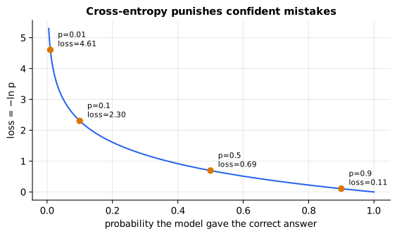
Reading it: the horizontal axis is how much probability the model put on the right answer; the vertical axis is the loss it pays. Start at the right edge: at p = 1 the loss is 0 and the curve is nearly flat, so going from 90% to 99% buys little. Now slide left: the curve bends sharply upward, and at p = 0.01 the loss is 4.61. The red dots are the table above. The shape is the whole story: small, diminishing rewards for being more right, and an unbounded bill for being confidently wrong.
The natural logarithm ln(p) answers "e to what power gives p?" For a
probability between 0 and 1 the answer is negative (ln 0.5 = −0.69,
because e^−0.69 = 0.5), so we flip the sign to get a positive cost. (Every symbol used in these
lessons is built from zero in primer.notation.)
Level 3: the formula and its symbols
$$ \mathcal{L} = -\ln p_{\text{correct}} $$
Symbols
| Symbol | Meaning here | In the example |
|---|---|---|
| $\mathcal{L}$ | the loss for one prediction | 0.69 |
| $p_{\text{correct}}$ | probability the model gave to the right answer, between 0 and 1 | 0.5 |
| $\ln$ | natural logarithm: the power you'd raise $e \approx 2.718$ to, to get the input | $\ln 0.5 = -0.69$ |
| $-$ | flips the sign so the loss is positive |
In words: "the loss is minus the natural log of the probability the model gave the right answer."
With the numbers: $-\ln 0.5 = 0.69$; $-\ln 0.01 = 4.61$.
Level 3: in Python
In Python:
import math
p_correct = 0.5
# −ln p_correct
round(-math.log(p_correct), 2)  # → 0.69
# confidently wrong costs far more
round(-math.log(0.01), 2)  # → 4.61
cross_entropy_from_prob is this one line.
Why it matters: a language model predicts the next token by choosing among its whole vocabulary, so this is the pretraining loss of every LLM. The steep penalty for confident mistakes is what pushes models toward calibrated probabilities.
From logits: the numerically safe way
A model doesn't output probabilities directly. It outputs raw scores called
logits, which softmax turns into probabilities (raise e to each score,
divide by the total; see primer.ml.attention). Computing that literally is
like measuring everyone's height in millimetres from the centre of the
Earth: the numbers get astronomically large and your calculator overflows.
Measure relative to the tallest person instead, and every number stays
small. That trick is log-sum-exp.
Worked example: logits (2, 1, 0.1), correct class 0. e² + e¹ + e^0.1 = 7.389 + 2.718 + 1.105 = 11.212, ln 11.212 = 2.417, so the loss is 2.417 − 2 = 0.417. And with logits (1000, 0) and class 1 correct, e^1000 overflows any computer, but log-sum-exp gives exactly 1000 − 0 = 1000.
flowchart LR
  Z[Logits z<br/>one score per class] --> M[Subtract max m]
  M --> LSE[log-sum-exp<br/>m + ln sum e^z-m]
  LSE --> L[Loss = LSE minus z_correct]
  Z --> L
  L -.backward.-> G[Gradient = softmax z<br/>minus one-hot target]
  G -.-> U[Raise the right logit,<br/>lower the others by their probability]
Reading it: solid arrows are the forward pass, dotted arrows the backward pass. The logits never go through an explicit softmax on the way forward: the largest logit is subtracted first so no exponent can overflow, and the loss is "log of the total" minus "the right class's score". Coming back, the gradient for every class is its predicted probability, minus 1 for the correct class. So the right logit is pushed up by (1 − p), and each wrong logit is pushed down by exactly the probability it took.
Level 3: the formula and its symbols
$$ -\ln \text{softmax}(z)_y = \ln \sum_j e^{z_j} - z_y, \qquad \ln \sum_j e^{z_j} = m + \ln \sum_j e^{z_j - m},\; m = \max_j z_j $$
Symbols
| Symbol | Meaning here | In the example |
|---|---|---|
| $z$ | the logits, one raw score per class | (2, 1, 0.1) |
| $z_j$ | the score of class $j$ | $z_0 = 2$ |
| $y$ | the index of the correct class | 0 |
| $\text{softmax}(z)_y$ | the probability softmax gives the correct class | 7.389 / 11.212 = 0.659 |
| $\sum_j$ | "add up over every class $j$" | three terms |
| $e^{z_j}$ | e ≈ 2.718 raised to the score | $e^2 = 7.389$ |
| $m$ | the largest logit, subtracted for safety | 2 |
| $\max_j$ | "the biggest value over all $j$" | 2 |
In words: "the loss is the log of the sum of e-to-every-score, minus the correct class's score; to compute that log safely, pull the biggest score out front first."
With the numbers: $m = 2$; $\sum_j e^{z_j - 2} = e^0 + e^{-1} + e^{-1.9} = 1 + 0.368 + 0.150 = 1.518$; $\ln 1.518 = 0.417$; so log-sum-exp $= 2.417$ and the loss is $2.417 - 2 = 0.417$ (and $-\ln 0.659 = 0.417$ too).
Level 3: in Python
In Python:
import math
def log_sum_exp(z):
    # m = max_j z_j
    m = max(z)
    # m + ln Σ_j e^(z_j − m)
    return m + math.log(sum(math.exp(z_j - m) for z_j in z))
z, y = [2.0, 1.0, 0.1], 0
round(log_sum_exp(z), 3)  # → 2.417
# ln Σ_j e^(z_j) − z_y
round(log_sum_exp(z) - z[y], 3)  # → 0.417
z, y = [1000.0, 0.0], 1
# e^1000 is never computed: no overflow
log_sum_exp(z) - z[y]  # → 1000.0
The gradient, which is how each logit should move:
Level 3: the formula and its symbols
$$ \frac{\partial \mathcal{L}}{\partial z} = \text{softmax}(z) - \text{onehot}(y) $$
Symbols
| Symbol | Meaning here | In the example |
|---|---|---|
| $\partial \mathcal{L} / \partial z$ | the gradient: one slope per logit | (0.25, −0.25) |
| $\text{softmax}(z)$ | the predicted probabilities | (0.25, 0.75) for logits (0, ln 3) |
| $\text{onehot}(y)$ | 1 at the correct class, 0 elsewhere | (0, 1) |
In words: "each logit's slope is its predicted probability, minus one if it's the right answer."
With the numbers: logits (0, ln 3) give softmax (1/4, 3/4); with class 1 correct, the gradient is (0.25 − 0, 0.75 − 1) = (0.25, −0.25).
Level 3: in Python
In Python:
import math
z, y = [0.0, math.log(3)], 1
exps = [math.exp(z_j) for z_j in z]
# (1/4, 3/4)
softmax = [e / sum(exps) for e in exps]
# (0, 1)
onehot = [1 if j == y else 0 for j in range(len(z))]
# softmax(z) − onehot(y)
[round(s_j - o_j, 2) for s_j, o_j in zip(softmax, onehot)]  # → [0.25, -0.25]
In code: log_sum_exp pulls the largest logit out front, log_softmax
subtracts that total from every logit, and softmax_cross_entropy returns
the batch's mean loss together with its softmax − onehot gradient.
Why it matters: this is why every framework fuses softmax and
cross-entropy into one operation that takes logits
(torch.nn.functional.cross_entropy). Computing softmax first and then the
log is the classic source of NaN losses.
Perplexity: how many options is the model torn between?
Imagine a game show with doors, one hiding the prize. If the model is as unsure as someone picking between two doors at random, its perplexity is 2; between ten doors, 10. Perplexity converts an average loss back into that "number of doors".
Worked example: a model that gives the right token 50% every time has loss 0.69 per token and perplexity e^0.69 = 2. One that gives 10% every time has perplexity 10. Three confident tokens (0.9) and one disaster (0.001) give perplexity about 6: one bad guess drags the whole average.
flowchart LR
  P["Per-token probabilities<br/>0.5, 0.5, 0.5"] --> NL["−ln each<br/>0.69, 0.69, 0.69"]
  NL --> AV["Average<br/>0.69"]
  AV --> EX["e to that power<br/>e^0.69 = 2"]
  EX --> D["≈ choosing between<br/>2 equally likely doors"]
Reading it: start with the probability the model gave each correct token, turn each into a loss with −ln, average them, then undo the log with e^x. The result is back in "number of options" units.
Level 3: the formula and its symbols
$$ \text{PPL} = \exp\left(\frac{1}{N}\sum_{i=1}^{N} -\ln p_i\right) $$
Symbols
| Symbol | Meaning here | In the example |
|---|---|---|
| $\text{PPL}$ | perplexity | 2 |
| $N$ | number of tokens | 3 |
| $i$ | a counter over the tokens | 1, 2, 3 |
| $p_i$ | probability given to the correct token at position $i$ | 0.5 each |
| $\frac{1}{N}\sum_{i=1}^{N}$ | "the average over all $N$ tokens" | $(0.69 + 0.69 + 0.69)/3$ |
| $\exp(x)$ | another way to write $e^x$ | $e^{0.69}$ |
In words: "perplexity is e raised to the average cross-entropy per token."
With the numbers: $\exp\left(\frac{1}{3}(0.69 \times 3)\right) = e^{0.69} = 2.0$.
Level 3: in Python
In Python:
import math
p = [0.5, 0.5, 0.5]
N = len(p)
# (1/N) Σ −ln p_i
average = sum(-math.log(p_i) for p_i in p) / N
round(average, 2)  # → 0.69
# exp(...)
round(math.exp(average), 1)  # → 2.0
In code: perplexity averages cross_entropy_from_prob over the tokens
and raises e to the result.
Why it matters: perplexity is the standard training metric for language models. It's comparable only between models that use the same tokenizer on the same text, and it says nothing direct about whether answers are helpful or correct.
Regression losses: fines for being off by an amount
When the prediction is a number (a price, a temperature), think of fines for arriving late. MAE (mean absolute error) is a flat rate: every minute late costs the same. MSE (mean squared error) squares the minutes: 10 minutes late costs 100, not 10, so one very late arrival outweighs many slightly late ones.
Worked example: four predictions miss by 1 and one misses by 10. MSE = (1 + 1 + 1 + 1 + 100) / 5 = 20.8, and the outlier is 100/104 = 96% of it. MAE = (1 + 1 + 1 + 1 + 10) / 5 = 2.8, and the outlier is 10/14 = 71%.
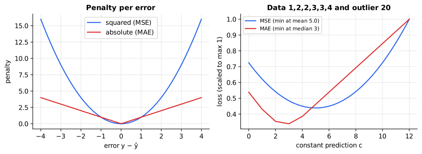
Reading it: the left panel is the price of a single error. Near zero the two curves are similar, but past an error of 1 the squared penalty climbs away from the absolute one. The right panel asks: if the model could predict only one constant for the data 1, 2, 2, 3, 3, 4 plus an outlier of 20, which constant minimizes each loss? MSE's valley sits at the mean (5.0), dragged right by the outlier; MAE's valley sits at the median (3), where most of the data is.
Level 3: the formula and its symbols
$$ \text{MSE} = \frac{1}{N}\sum_{i=1}^{N}(y_i - \hat{y}_i)^2, \qquad \text{MAE} = \frac{1}{N}\sum_{i=1}^{N}\lvert y_i - \hat{y}_i\rvert $$
Symbols
| Symbol | Meaning here | In the example |
|---|---|---|
| $N$ | number of predictions | 5 |
| $y_i$ | the true value for example $i$ | 0 for all five |
| $\hat{y}_i$ | "y-hat", the predicted value | 1, −1, 1, −1, 10 |
| $y_i - \hat{y}_i$ | the error (residual) | −1, 1, −1, 1, −10 |
| $(\cdot)^2$ | square: multiply by itself (always positive) | $(-10)^2 = 100$ |
| $\lvert\cdot\rvert$ | absolute value: drop the sign | $\lvert -10\rvert = 10$ |
In words: "MSE is the average of the squared errors; MAE is the average of the errors ignoring their sign."
With the numbers: MSE $= (1+1+1+1+100)/5 = 20.8$; MAE $= (1+1+1+1+10)/5 = 2.8$.
Level 3: in Python
In Python:
y = [0, 0, 0, 0, 0]
y_hat = [1, -1, 1, -1, 10]
N = len(y)
# MSE
sum((y_i - y_hat_i) ** 2 for y_i, y_hat_i in zip(y, y_hat)) / N  # → 20.8
# MAE
sum(abs(y_i - y_hat_i) for y_i, y_hat_i in zip(y, y_hat)) / N  # → 2.8
In code: mse and mae are the two averages, and outlier_share
measures how much of each total the single largest error contributes (the
96% and 71% above).
Why it matters: pick the loss whose valley is where you want your predictions. MSE chases outliers (its best constant is the mean); MAE shrugs them off (its best constant is the median). For noisy data with occasional wild values, MAE or a blend (Huber loss) is safer.
Contrastive loss (InfoNCE): find your partner in a crowd
Picture a party game. Everyone arrives in pairs, gets separated, and must pick their partner out of the whole room. Everyone else in the room is a decoy. A contrastive loss scores how confidently each person picks their own partner over every decoy. The hardest decoy is your partner's lookalike twin: same topic, wrong person. That's a hard negative.
Embedding models (and CLIP) learn this way: a query and the passage that answers it are "partners"; the other passages in the same batch are free decoys (in-batch negatives).
Worked example: two queries and two passages, as vectors, scored with the dot product (multiply matching entries, add them up). Query 1 = (1, 0), query 2 = (0, 1), passage 1 = (1, 0), passage 2 = (0, 1), temperature 1. Query 1 scores 1 against its partner and 0 against the decoy. Its loss is −ln(e¹ / (e¹ + e⁰)) = ln(1 + e^−1) = 0.3133. Swap the passages and each query now prefers the decoy: the loss rises to ln(1 + e¹) = 1.3133.
flowchart LR
  Q[Batch of queries] --> S[Score matrix<br/>every query vs every passage]
  D[Their matching passages] --> S
  S --> CE[Cross-entropy per row<br/>right answer = the diagonal]
  CE --> L[Pull pairs together<br/>push the rest apart]
Reading it: a batch of queries and the passages that answer them are turned into vectors, then every query is scored against every passage, giving a square grid. Each row becomes a classification ("which of these passages is mine?") whose right answer is on the diagonal. Cross-entropy on those rows pulls each query toward its own passage and away from all the others at once.
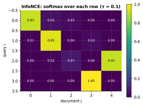
Reading it: rows are queries, columns are passages, and each cell is the probability that query i "picks" passage j. A well-trained model shows a bright diagonal. Look at row 2: it puts most of its probability on column 4, an extra mined hard negative built to resemble query 2, and only a few percent on its own passage (column 2). The model is fooled, and that row is exactly where the loss, and therefore the gradient, concentrates. Rows 0, 1 and 3 are already confident and contribute almost nothing to learning.
Level 3: the formula and its symbols
$$ \mathcal{L}_i = -\ln \frac{\exp(q_i \cdot d_i / \tau)}{\sum_{j=1}^{N} \exp(q_i \cdot d_j / \tau)} $$
Symbols
| Symbol | Meaning here | In the example |
|---|---|---|
| $\mathcal{L}_i$ | the loss for query $i$ | 0.3133 |
| $q_i$ | query $i$'s vector | $q_1 = (1, 0)$ |
| $d_i$ | query $i$'s own passage (its positive) | $d_1 = (1, 0)$ |
| $d_j$ | passage $j$: every passage in the batch, the positive included | $d_1, d_2$ |
| $q_i \cdot d_j$ | dot product: how aligned query and passage are | $q_1 \cdot d_1 = 1$, $q_1 \cdot d_2 = 0$ |
| $\tau$ | "tau", the temperature: divides scores; small $\tau$ sharpens, large softens | 1 |
| $N$ | number of passages scored (batch plus any extra negatives) | 2 |
| $\exp$ | $e$ raised to the power | $e^1 = 2.718$ |
In words: "for each query, take e-to-the-score of its own passage, divide by the sum of e-to-the-score over every passage in the batch, and charge minus the log of that share."
With the numbers: $-\ln \frac{e^{1}}{e^{1} + e^{0}} = -\ln \frac{2.718}{3.718} = -\ln 0.731 = 0.3133$. At temperature 0.1 the same vectors give $-\ln \frac{e^{10}}{e^{10} + 1} \approx 0.000045$: sharper.
Level 3: in Python
In Python:
import math
# the queries
q = [[1, 0], [0, 1]]
# their passages: d[i] is q[i]'s partner
d = [[1, 0], [0, 1]]
def dot(a, b):
    return sum(a_k * b_k for a_k, b_k in zip(a, b))
def info_nce(i, tau):
    # exp(q_i · d_j / τ) for every j
    scores = [math.exp(dot(q[i], d_j) / tau) for d_j in d]
    # −ln (own passage's share)
    return -math.log(scores[i] / sum(scores))
round(info_nce(0, tau=1.0), 4)  # → 0.3133
print(f"{info_nce(0, tau=0.1):.6f}")  # → 0.000045
It's just cross-entropy where the "classes" are the passages in the batch, so the gradient is the same softmax − onehot, pushed back through the dot products into both sets of vectors.
In code: info_nce builds the score grid, hands it to
softmax_cross_entropy with the diagonal as the right answers, and returns
the gradients for both sets of vectors; info_nce_gradient_check confirms
those gradients against small nudges of every number.
Why it matters: this is how search and RAG embedding models are trained
(see primer.ml.embeddings.contrastive). Bigger batches mean more free
negatives. Easy negatives are already far away and contribute almost no
gradient; hard negatives produce most of the learning signal, which is why
mining them is the biggest lever on retrieval quality.
Label smoothing: never say 100%
A good forecaster never says "100% chance of rain", because the one day they're wrong would be infinitely embarrassing. Label smoothing teaches the model the same humility: instead of "the answer is class 2, with total certainty", the target says "class 2, with 92.5% certainty, and a sliver of doubt spread over everything".
Worked example: 4 classes, correct class 2, smoothing ε = 0.1. Take 0.9 of the one-hot target (0, 0, 0.9, 0) and add 0.1/4 = 0.025 to every class: (0.025, 0.025, 0.925, 0.025). A model that puts logit 50 on the right class has plain cross-entropy ≈ 0, but smoothed cross-entropy 3 × 0.025 × 50 = 3.75.
flowchart LR
  O[One-hot target<br/>0, 0, 1, 0] --> MIX[Mix: 1 minus eps times one-hot<br/>plus eps/K everywhere]
  U[Uniform over K classes] --> MIX
  MIX --> T[Soft target<br/>0.025, 0.025, 0.925, 0.025]
  T --> CE[Cross-entropy against<br/>the soft target]
Reading it: the hard one-hot label and a uniform distribution are blended with weight ε, giving a target that is still 92.5% sure but never 100%. Training against it means the loss can never reach zero, so the model gains nothing by pushing its logits toward infinity.
Level 3: the formula and its symbols
$$ t = (1 - \varepsilon)\,\text{onehot}(y) + \frac{\varepsilon}{K}, \qquad \mathcal{L} = -\sum_{k=1}^{K} t_k \ln \text{softmax}(z)_k $$
Symbols
| Symbol | Meaning here | In the example |
|---|---|---|
| $t$ | the smoothed target distribution | (0.025, 0.025, 0.925, 0.025) |
| $\varepsilon$ | "epsilon", how much certainty to give away | 0.1 |
| $K$ | number of classes | 4 |
| $k$ | a counter over the classes | 1 to 4 |
| $t_k$ | target weight on class $k$ | 0.925 on the right class |
| $\text{softmax}(z)_k$ | predicted probability of class $k$ | ≈1 on the right class |
In words: "the target keeps (1 − ε) on the right answer and spreads ε evenly over all classes; the loss is cross-entropy against that softer target."
With the numbers: $(1 - 0.1) \cdot 1 + 0.1/4 = 0.925$ on the right class and $0.025$ elsewhere; with logits (0, 0, 50, 0) the three wrong classes each have $\ln \text{softmax} \approx -50$, so $\mathcal{L} \approx 3 \times 0.025 \times 50 = 3.75$.
Level 3: in Python
In Python:
import math
eps, K, y = 0.1, 4, 2
# t_k
t = [(1 - eps) * (1 if k == y else 0) + eps / K for k in range(K)]
[round(t_k, 3) for t_k in t]  # → [0.025, 0.025, 0.925, 0.025]
z = [0.0, 0.0, 50.0, 0.0]
m = max(z)
log_total = m + math.log(sum(math.exp(z_k - m) for z_k in z))
# ln softmax(z)_k
log_softmax = [z_k - log_total for z_k in z]
# −Σ_k t_k ln softmax(z)_k
round(-sum(t_k * ls_k for t_k, ls_k in zip(t, log_softmax)), 2)  # → 3.75
In code: smoothed_targets builds the soft target t, and
smoothed_cross_entropy scores the logits against it.
Why it matters: it curbs over-confidence and often improves calibration (how well the model's stated confidence matches how often it's right). It was used to train the original transformer.
In 20 seconds
- Cross-entropy is −ln(probability on the right answer): small when confident and right, huge when confident and wrong.
- Perplexity = e^(average cross-entropy): the effective number of choices per token.
- Compute it from logits with log-sum-exp; its gradient is softmax − onehot.
- MSE punishes big misses (mean); MAE is robust to outliers (median).
- Contrastive (InfoNCE) loss is cross-entropy over "which passage in this batch is mine?"; hard negatives drive retrieval quality.
Self-test questions
The model puts 1% on the right token. What's the loss, and why so large? −ln(0.01) = 4.61, about 44× the loss at 90% (0.105). The log punishes confident mistakes steeply, which pushes the model toward calibrated probabilities.
Loss is 0.69 per token. What's the perplexity? e^0.69 = 2: as uncertain as a coin flip between two options.
Why compute cross-entropy from logits instead of from softmax outputs? Softmax of large logits overflows, and the log of a tiny probability underflows to −∞. Log-sum-exp subtracts the max first and never exponentiates a large number. The fused gradient is simply softmax − onehot.
When would you pick MAE over MSE? When outliers are noise you don't want to chase. MSE squares errors, so one huge miss dominates; MAE weighs errors linearly.
How does InfoNCE get negatives without labelling them? It uses the other items in the batch: for each query, every other query's positive passage is a negative. Bigger batches mean more (and harder) negatives for free.
Why do hard negatives matter? Easy negatives are already far away and contribute almost no gradient. Hard negatives score high and produce most of the learning signal, teaching the model to separate "on topic" from "actually answers the question".
The papers behind this lesson
- van den Oord, Li & Vinyals, Representation Learning with Contrastive Predictive Coding (2018): https://arxiv.org/abs/1807.03748 Named and analysed InfoNCE, the "pick the positive out of N" contrastive loss.
- Chen et al., A Simple Framework for Contrastive Learning of Visual Representations (SimCLR, 2020): https://arxiv.org/abs/2002.05709 Showed how much in-batch negatives, large batches and the temperature matter for contrastive training.
- Radford et al., Learning Transferable Visual Models From Natural Language Supervision (CLIP, 2021): https://arxiv.org/abs/2103.00020 Trained image and text encoders with a symmetric InfoNCE loss on 400 million pairs, putting both in one vector space. annotated companion
- Szegedy et al., Rethinking the Inception Architecture for Computer Vision (2015): https://arxiv.org/abs/1512.00567 Introduced label smoothing as a regularizer against over-confident predictions.
Further reading
- Goodfellow, Bengio & Courville, Deep Learning, ch. 6 (cost functions): https://www.deeplearningbook.org/contents/mlp.html
- CS231n notes, Linear classification (softmax and cross-entropy): https://cs231n.github.io/linear-classify/
- PyTorch
cross_entropy: https://pytorch.org/docs/stable/generated/torch.nn.functional.cross_entropy.html - van den Oord et al., Representation Learning with Contrastive Predictive Coding (InfoNCE, 2018): https://arxiv.org/abs/1807.03748
- Chen et al., SimCLR (in-batch negatives and temperature, 2020): https://arxiv.org/abs/2002.05709
- Radford et al., CLIP (2021): https://arxiv.org/abs/2103.00020
- Szegedy et al., Rethinking the Inception Architecture (label smoothing, 2015): https://arxiv.org/abs/1512.00567
- Müller et al., When Does Label Smoothing Help? (2019): https://arxiv.org/abs/1906.02629
1r""" 2# Loss functions: turning "how wrong were we?" into one number 3 4Run: `python -m primer.ml.losses` 5 6New to the notation? `primer.notation` explains every symbol used here from 7zero. This lesson builds on the training loop from `primer.ml.neural_net`. 8 9## Level 1: The practitioner's guide 10 11**In one sentence.** A loss function turns "how wrong was this prediction?" 12into one number that training pushes down, and because the model learns 13whatever that number rewards, choosing the loss is choosing the behaviour. 14 15**When you need it.** Every time you train or fine-tune anything, the first 16line of the job is the loss, and every time you read a training curve, a 17model card's perplexity or a fine-tuning API's "training loss" you are 18reading one. The tell that you have the wrong loss, or are reading one 19wrongly: the loss goes down and the thing you care about does not, or one 20example is most of the number. This lesson's regression example shows how 21easily that happens: four predictions off by 1 and one off by 10 give a mean 22squared error of 20.8, of which the single outlier is 96%; the mean absolute 23error is 2.8 and the outlier is 71% of it. In language modelling, three 24tokens at 0.9 and one at 0.001 give a perplexity of 6.09, when the three 25good tokens alone would give about 1.1 (this lesson's `perplexity`). You 26don't need this lesson while you only prompt a hosted model: the vendor 27chose the loss years ago. You need it the day you fine-tune, train an 28embedding model, or have to explain why a loss of 0.69 is a coin flip. 29 30**Your options.** The losses practice reaches for, by what the model 31predicts: 32 33| Option | For predicting | What it pushes the model toward | What its number hides | Where it lives | 34|---|---|---|---|---| 35| Cross-entropy | a class, or the next token | Putting probability on the right answer; a confident miss (1%) costs 44 times a mostly-right one (90%) | An average over tokens, so one catastrophic token dominates the mean | Every classifier, and the pretraining and fine-tuning of every language model | 36| Perplexity (a reading of cross-entropy, not a loss) | the same | Nothing new: it is e raised to the mean loss, "how many doors is the model choosing between" | Whether answers are correct or helpful; comparable only across the same tokenizer and text | Model cards, training dashboards | 37| Mean squared error (MSE) | a number | The mean of the targets; big misses are squared, so the model chases them | A few wild values (96% of the number above) | Regression heads, forecasting, any "predict a quantity" model | 38| Mean absolute error (MAE) | a number | The median; every unit of miss costs the same | How large the largest misses are | The same jobs, when the targets have noise you do not want chased | 39| Huber loss | a number | MSE near zero, MAE far out: a blend | One more knob, the crossover point | Frameworks' regression losses | 40| Contrastive (InfoNCE) | which items belong together | Picking each query's partner out of the batch, every other item a free decoy | Easy rows contribute almost nothing; a hard negative can be most of the loss | Embedding models for search and RAG, CLIP | 41| Label smoothing (a modifier on cross-entropy) | classes or tokens | Never saying 100%: with ε = 0.1 over 4 classes the target is 92.5% on the right answer | The loss can no longer reach zero, so the floor moves | Classifiers, the original transformer | 42 43**How to choose.** Start from what the model outputs, then ask what a wrong 44answer costs you. 45 46- A class or the next token: cross-entropy, computed from the raw scores 47 (logits) in one fused operation. Never take the softmax and then the log 48 yourself; that is the classic source of a loss that reads NaN. 49- A number: decide whether an outlier is signal or noise. If the wild 50 values are real and expensive, MSE chases them for you; if they are bad 51 labels or rare accidents, MAE shrugs them off; when you cannot tell, Huber. 52- Pairs that belong together (a question and the passage that answers it, 53 an image and its caption): InfoNCE with the largest batch you can afford, 54 then mine hard negatives, because that is where the gradient is. 55- A classifier that is confidently wrong too often, or a generator you will 56 decode with beam search: add label smoothing with ε around 0.1. 57- Whatever you pick, the loss is what the model optimises and the metric 58 (`primer.ml.metrics`) is what you care about. Keep both on the same 59 dashboard, and when they disagree, believe the metric. 60 61**What it costs.** Compute is not the cost; a loss is a few operations 62next to a forward pass, and the safe cross-entropy is a max, a sum and one 63logarithm. The real costs are elsewhere. InfoNCE scores every query against 64every passage in the batch, so a batch of N costs an N-by-N grid and the 65number of free negatives is the batch size: memory buys signal, and SimCLR 66reports that contrastive learning wants larger batches and more steps than 67supervised training does. Label smoothing costs nothing at inference and 68raises the loss you will see in training: in this lesson a model that puts 69logit 50 on the right class scores 0 under plain cross-entropy and 3.75 70under smoothing, which is the point. Perplexity is free, being arithmetic 71on a loss you already have. The expensive mistake is choosing a loss that 72optimises the wrong thing and only finding out at evaluation, after the GPU 73bill: MSE on data with a few wild labels moves the model's best constant 74guess from the median 3 to the mean 5 in this lesson's figure. 75 76**What breaks.** 77 78- **NaN or infinite loss.** Softmax then log overflows on large logits and 79 underflows on tiny probabilities. Use the fused version that subtracts the 80 largest logit first (`primer.ml.losses` builds it as `log_sum_exp`). 81- **Loss falls, quality doesn't.** Cross-entropy pays for probability on the 82 reference text, not for a correct or useful answer. A model can lower its 83 perplexity by matching style while getting facts wrong. Evaluate with a 84 metric that reads the answer. 85- **One example is the whole number.** Look at the distribution of 86 per-example losses, not only the mean. A 96% outlier share in MSE means 87 the gradient is almost entirely one row. 88- **Perplexity across models.** A number from a different tokenizer, or on 89 different text, is not comparable. Compare within one setup. 90- **A contrastive loss that stalls.** In this lesson's 4-row batch three 91 rows contribute 0.087, 0.048 and 0.004 while the row with a mined hard 92 negative contributes 2.694. If your batch has no hard rows, the model has 93 nothing left to learn from it; mine harder negatives or grow the batch. 94- **The wrong temperature.** The same two perfectly matched vectors give an 95 InfoNCE loss of 0.3133 at temperature 1 and 0.000045 at 0.1. Too low and 96 the loss saturates on easy pairs; the temperature (or "scale") is a real 97 hyperparameter, not a default to inherit. 98- **Smoothing a teacher.** Müller, Kornblith and Hinton (2019) report that 99 label smoothing improves calibration but makes a smoothed model a much 100 worse teacher for distillation. Skip it on a model you will distil from. 101 102**In the wild.** PyTorch's `torch.nn.functional.cross_entropy` takes 103"predicted unnormalized logits" and has a `label_smoothing` argument, so 104both the fused computation and the modifier are one call. A hosted fine-tuning API's 105"training loss" is this cross-entropy, graded on the reply tokens only 106(`primer.ml.training_stages`). Perplexity is the number on 107language-model training dashboards and, still, on many model cards. In 108retrieval, sentence-transformers' `MultipleNegativesRankingLoss` is InfoNCE 109with in-batch negatives and optional mined hard negatives per query, and its 110documentation describes the scale (the inverse temperature) as a parameter. 111CLIP trained its image and text encoders with a symmetric InfoNCE loss on 112400 million pairs, and SimCLR measured how much the batch size and the 113temperature matter. Label smoothing was used to train the original 114transformer. 115 116**Go deeper.** Level 2 builds each of these from nothing: the −ln p curve 117and why a 1% miss costs 44 times a 90% hit, log-sum-exp and the one-line 118gradient "softmax minus one-hot", perplexity as a count of doors, the 119valleys of MSE and MAE on a toy dataset, the InfoNCE score grid with a 120gradient check, and label smoothing's soft target, every number rerunnable. 121If you only needed to choose a loss and read its number, you are done. 122 123## Level 2: How it works, from scratch 124 125A loss is a scorecard with one number on it. Imagine a coach who, after every 126practice, must summarise the whole team's performance in a single score so 127the players know whether they're improving. Training a model does exactly 128this: it computes the loss, then adjusts the weights to make that number 129smaller (see `primer.ml.neural_net` for the loop). 130 131What the scorecard rewards is what the model learns. Language models are 132scored on how much probability they gave the real next word; price 133predictors on how far off their numbers were; search models on whether they 134ranked the right passage above the wrong ones. 135 136```mermaid 137flowchart LR 138 P[Prediction] --> LF{Loss function} 139 T[Right answer] --> LF 140 LF -->|classes or tokens| CE[Cross-entropy] 141 LF -->|numbers| REG[MSE or MAE] 142 LF -->|matching pairs| CON[Contrastive / InfoNCE] 143 CE & REG & CON --> N[One number to minimize] 144``` 145 146**Reading it:** a prediction and the right answer go into the loss function 147and one number comes out. Which branch you take depends on what the model 148predicts: a choice among classes (or the next token) uses cross-entropy, a 149number uses squared or absolute error, and "which of these belong together" 150uses a contrastive loss. Each section below climbs one branch. 151 152## Cross-entropy: how surprised were we by the truth? 153 154Picture a weather forecaster scored every evening. If they said "90% chance 155of rain" and it rained, they lose a point or two. If they said "1% chance of 156rain" and it poured, they are humiliated. Cross-entropy is that humiliation 157meter: it charges according to how little probability you gave to what 158actually happened. 159 160Worked example: the model assigned these probabilities to the correct next 161token. 162 163| Probability on the correct token | Loss (−ln p) | 164|---|---| 165| 0.9 | 0.11 | 166| 0.5 | 0.69 | 167| 0.1 | 2.30 | 168| 0.01 | 4.61 | 169 170Being confidently wrong (1%) costs about **44×** more than being mostly 171right (90%): 4.61 / 0.105 ≈ 44. 172 173 174 175**Reading it:** the horizontal axis is how much probability the model put on 176the right answer; the vertical axis is the loss it pays. Start at the right 177edge: at p = 1 the loss is 0 and the curve is nearly flat, so going from 90% 178to 99% buys little. Now slide left: the curve bends sharply upward, and at 179p = 0.01 the loss is 4.61. The red dots are the table above. The shape is the 180whole story: small, diminishing rewards for being more right, and an 181unbounded bill for being confidently wrong. 182 183The **natural logarithm** ln(p) answers "e to what power gives p?" For a 184probability between 0 and 1 the answer is negative (ln 0.5 = −0.69, 185because e^−0.69 = 0.5), so we flip the sign to get a positive cost. (Every symbol used in these 186lessons is built from zero in `primer.notation`.) 187 188$$ 189\mathcal{L} = -\ln p_{\text{correct}} 190$$ 191 192**Symbols** 193 194| Symbol | Meaning here | In the example | 195|---|---|---| 196| $\mathcal{L}$ | the loss for one prediction | 0.69 | 197| $p_{\text{correct}}$ | probability the model gave to the right answer, between 0 and 1 | 0.5 | 198| $\ln$ | natural logarithm: the power you'd raise $e \approx 2.718$ to, to get the input | $\ln 0.5 = -0.69$ | 199| $-$ | flips the sign so the loss is positive | | 200 201**In words:** "the loss is minus the natural log of the probability the 202model gave the right answer." 203 204**With the numbers:** $-\ln 0.5 = 0.69$; $-\ln 0.01 = 4.61$. 205 206**In Python:** 207 208```python 209import math 210p_correct = 0.5 211# −ln p_correct 212round(-math.log(p_correct), 2) # → 0.69 213# confidently wrong costs far more 214round(-math.log(0.01), 2) # → 4.61 215``` 216 217`cross_entropy_from_prob` is this one line. 218 219**Why it matters:** a language model predicts the next token by choosing 220among its whole vocabulary, so this *is* the pretraining loss of every LLM. 221The steep penalty for confident mistakes is what pushes models toward 222calibrated probabilities. 223 224## From logits: the numerically safe way 225 226A model doesn't output probabilities directly. It outputs raw scores called 227**logits**, which softmax turns into probabilities (raise *e* to each score, 228divide by the total; see `primer.ml.attention`). Computing that literally is 229like measuring everyone's height in millimetres from the centre of the 230Earth: the numbers get astronomically large and your calculator overflows. 231Measure relative to the tallest person instead, and every number stays 232small. That trick is **log-sum-exp**. 233 234Worked example: logits (2, 1, 0.1), correct class 0. 235e² + e¹ + e^0.1 = 7.389 + 2.718 + 1.105 = 11.212, ln 11.212 = 2.417, so the 236loss is 2.417 − 2 = **0.417**. And with logits (1000, 0) and class 1 correct, 237e^1000 overflows any computer, but log-sum-exp gives exactly 1000 − 0 = **1000**. 238 239```mermaid 240flowchart LR 241 Z[Logits z<br/>one score per class] --> M[Subtract max m] 242 M --> LSE[log-sum-exp<br/>m + ln sum e^z-m] 243 LSE --> L[Loss = LSE minus z_correct] 244 Z --> L 245 L -.backward.-> G[Gradient = softmax z<br/>minus one-hot target] 246 G -.-> U[Raise the right logit,<br/>lower the others by their probability] 247``` 248 249**Reading it:** solid arrows are the forward pass, dotted arrows the backward 250pass. The logits never go through an explicit softmax on the way forward: 251the largest logit is subtracted first so no exponent can overflow, and the 252loss is "log of the total" minus "the right class's score". Coming back, the 253gradient for every class is its predicted probability, minus 1 for the 254correct class. So the right logit is pushed up by (1 − p), and each wrong 255logit is pushed down by exactly the probability it took. 256 257$$ 258-\ln \text{softmax}(z)_y = \ln \sum_j e^{z_j} - z_y, 259\qquad 260\ln \sum_j e^{z_j} = m + \ln \sum_j e^{z_j - m},\; m = \max_j z_j 261$$ 262 263**Symbols** 264 265| Symbol | Meaning here | In the example | 266|---|---|---| 267| $z$ | the logits, one raw score per class | (2, 1, 0.1) | 268| $z_j$ | the score of class $j$ | $z_0 = 2$ | 269| $y$ | the index of the correct class | 0 | 270| $\text{softmax}(z)_y$ | the probability softmax gives the correct class | 7.389 / 11.212 = 0.659 | 271| $\sum_j$ | "add up over every class $j$" | three terms | 272| $e^{z_j}$ | *e* ≈ 2.718 raised to the score | $e^2 = 7.389$ | 273| $m$ | the largest logit, subtracted for safety | 2 | 274| $\max_j$ | "the biggest value over all $j$" | 2 | 275 276**In words:** "the loss is the log of the sum of e-to-every-score, minus the 277correct class's score; to compute that log safely, pull the biggest score 278out front first." 279 280**With the numbers:** $m = 2$; $\sum_j e^{z_j - 2} = e^0 + e^{-1} + e^{-1.9} = 2811 + 0.368 + 0.150 = 1.518$; $\ln 1.518 = 0.417$; so log-sum-exp $= 2.417$ and the 282loss is $2.417 - 2 = 0.417$ (and $-\ln 0.659 = 0.417$ too). 283 284**In Python:** 285 286```python 287import math 288def log_sum_exp(z): 289 # m = max_j z_j 290 m = max(z) 291 # m + ln Σ_j e^(z_j − m) 292 return m + math.log(sum(math.exp(z_j - m) for z_j in z)) 293z, y = [2.0, 1.0, 0.1], 0 294round(log_sum_exp(z), 3) # → 2.417 295# ln Σ_j e^(z_j) − z_y 296round(log_sum_exp(z) - z[y], 3) # → 0.417 297z, y = [1000.0, 0.0], 1 298# e^1000 is never computed: no overflow 299log_sum_exp(z) - z[y] # → 1000.0 300``` 301 302The gradient, which is how each logit should move: 303 304$$ 305\frac{\partial \mathcal{L}}{\partial z} = \text{softmax}(z) - \text{onehot}(y) 306$$ 307 308**Symbols** 309 310| Symbol | Meaning here | In the example | 311|---|---|---| 312| $\partial \mathcal{L} / \partial z$ | the gradient: one slope per logit | (0.25, −0.25) | 313| $\text{softmax}(z)$ | the predicted probabilities | (0.25, 0.75) for logits (0, ln 3) | 314| $\text{onehot}(y)$ | 1 at the correct class, 0 elsewhere | (0, 1) | 315 316**In words:** "each logit's slope is its predicted probability, minus one 317if it's the right answer." 318 319**With the numbers:** logits (0, ln 3) give softmax (1/4, 3/4); with class 1 320correct, the gradient is (0.25 − 0, 0.75 − 1) = (0.25, −0.25). 321 322**In Python:** 323 324```python 325import math 326z, y = [0.0, math.log(3)], 1 327exps = [math.exp(z_j) for z_j in z] 328# (1/4, 3/4) 329softmax = [e / sum(exps) for e in exps] 330# (0, 1) 331onehot = [1 if j == y else 0 for j in range(len(z))] 332# softmax(z) − onehot(y) 333[round(s_j - o_j, 2) for s_j, o_j in zip(softmax, onehot)] # → [0.25, -0.25] 334``` 335 336**In code:** `log_sum_exp` pulls the largest logit out front, `log_softmax` 337subtracts that total from every logit, and `softmax_cross_entropy` returns 338the batch's mean loss together with its softmax − onehot gradient. 339 340**Why it matters:** this is why every framework fuses softmax and 341cross-entropy into one operation that takes logits 342(`torch.nn.functional.cross_entropy`). Computing softmax first and then the 343log is the classic source of NaN losses. 344 345## Perplexity: how many options is the model torn between? 346 347Imagine a game show with doors, one hiding the prize. If the model is as 348unsure as someone picking between two doors at random, its perplexity is 2; 349between ten doors, 10. Perplexity converts an average loss back into that 350"number of doors". 351 352Worked example: a model that gives the right token 50% every time has loss 3530.69 per token and perplexity e^0.69 = 2. One that gives 10% every time has 354perplexity 10. Three confident tokens (0.9) and one disaster (0.001) give 355perplexity about 6: one bad guess drags the whole average. 356 357```mermaid 358flowchart LR 359 P["Per-token probabilities<br/>0.5, 0.5, 0.5"] --> NL["−ln each<br/>0.69, 0.69, 0.69"] 360 NL --> AV["Average<br/>0.69"] 361 AV --> EX["e to that power<br/>e^0.69 = 2"] 362 EX --> D["≈ choosing between<br/>2 equally likely doors"] 363``` 364 365**Reading it:** start with the probability the model gave each correct 366token, turn each into a loss with −ln, average them, then undo the log with 367e^x. The result is back in "number of options" units. 368 369$$ 370\text{PPL} = \exp\left(\frac{1}{N}\sum_{i=1}^{N} -\ln p_i\right) 371$$ 372 373**Symbols** 374 375| Symbol | Meaning here | In the example | 376|---|---|---| 377| $\text{PPL}$ | perplexity | 2 | 378| $N$ | number of tokens | 3 | 379| $i$ | a counter over the tokens | 1, 2, 3 | 380| $p_i$ | probability given to the correct token at position $i$ | 0.5 each | 381| $\frac{1}{N}\sum_{i=1}^{N}$ | "the average over all $N$ tokens" | $(0.69 + 0.69 + 0.69)/3$ | 382| $\exp(x)$ | another way to write $e^x$ | $e^{0.69}$ | 383 384**In words:** "perplexity is e raised to the average cross-entropy per 385token." 386 387**With the numbers:** $\exp\left(\frac{1}{3}(0.69 \times 3)\right) = e^{0.69} = 2.0$. 388 389**In Python:** 390 391```python 392import math 393p = [0.5, 0.5, 0.5] 394N = len(p) 395# (1/N) Σ −ln p_i 396average = sum(-math.log(p_i) for p_i in p) / N 397round(average, 2) # → 0.69 398# exp(...) 399round(math.exp(average), 1) # → 2.0 400``` 401 402**In code:** `perplexity` averages `cross_entropy_from_prob` over the tokens 403and raises e to the result. 404 405**Why it matters:** perplexity is the standard training metric for language 406models. It's comparable only between models that use the same tokenizer on 407the same text, and it says nothing direct about whether answers are 408helpful or correct. 409 410## Regression losses: fines for being off by an amount 411 412When the prediction is a number (a price, a temperature), think of fines for 413arriving late. **MAE** (mean absolute error) is a flat rate: every minute late 414costs the same. **MSE** (mean squared error) squares the minutes: 10 minutes 415late costs 100, not 10, so one very late arrival outweighs many slightly late 416ones. 417 418Worked example: four predictions miss by 1 and one misses by 10. 419MSE = (1 + 1 + 1 + 1 + 100) / 5 = **20.8**, and the outlier is 100/104 = 96% of 420it. MAE = (1 + 1 + 1 + 1 + 10) / 5 = **2.8**, and the outlier is 10/14 = 71%. 421 422 423 424**Reading it:** the left panel is the price of a single error. Near zero the 425two curves are similar, but past an error of 1 the squared penalty climbs 426away from the absolute one. The right panel asks: if the model could predict 427only one constant for the data 1, 2, 2, 3, 3, 4 plus an outlier of 20, which 428constant minimizes each loss? MSE's valley sits at the mean (5.0), dragged 429right by the outlier; MAE's valley sits at the median (3), where most of the 430data is. 431 432$$ 433\text{MSE} = \frac{1}{N}\sum_{i=1}^{N}(y_i - \hat{y}_i)^2, \qquad 434\text{MAE} = \frac{1}{N}\sum_{i=1}^{N}\lvert y_i - \hat{y}_i\rvert 435$$ 436 437**Symbols** 438 439| Symbol | Meaning here | In the example | 440|---|---|---| 441| $N$ | number of predictions | 5 | 442| $y_i$ | the true value for example $i$ | 0 for all five | 443| $\hat{y}_i$ | "y-hat", the predicted value | 1, −1, 1, −1, 10 | 444| $y_i - \hat{y}_i$ | the error (residual) | −1, 1, −1, 1, −10 | 445| $(\cdot)^2$ | square: multiply by itself (always positive) | $(-10)^2 = 100$ | 446| $\lvert\cdot\rvert$ | absolute value: drop the sign | $\lvert -10\rvert = 10$ | 447 448**In words:** "MSE is the average of the squared errors; MAE is the average 449of the errors ignoring their sign." 450 451**With the numbers:** MSE $= (1+1+1+1+100)/5 = 20.8$; MAE $= (1+1+1+1+10)/5 = 2.8$. 452 453**In Python:** 454 455```python 456y = [0, 0, 0, 0, 0] 457y_hat = [1, -1, 1, -1, 10] 458N = len(y) 459# MSE 460sum((y_i - y_hat_i) ** 2 for y_i, y_hat_i in zip(y, y_hat)) / N # → 20.8 461# MAE 462sum(abs(y_i - y_hat_i) for y_i, y_hat_i in zip(y, y_hat)) / N # → 2.8 463``` 464 465**In code:** `mse` and `mae` are the two averages, and `outlier_share` 466measures how much of each total the single largest error contributes (the 46796% and 71% above). 468 469**Why it matters:** pick the loss whose valley is where you want your 470predictions. MSE chases outliers (its best constant is the mean); MAE 471shrugs them off (its best constant is the median). For noisy data with 472occasional wild values, MAE or a blend (Huber loss) is safer. 473 474## Contrastive loss (InfoNCE): find your partner in a crowd 475 476Picture a party game. Everyone arrives in pairs, gets separated, and must 477pick their partner out of the whole room. Everyone else in the room is a 478decoy. A contrastive loss scores how confidently each person picks their own 479partner over every decoy. The hardest decoy is your partner's lookalike 480twin: same topic, wrong person. That's a **hard negative**. 481 482Embedding models (and CLIP) learn this way: a query and the passage that 483answers it are "partners"; the other passages in the same batch are free 484decoys (**in-batch negatives**). 485 486Worked example: two queries and two passages, as vectors, scored with the 487**dot product** (multiply matching entries, add them up). Query 1 = (1, 0), 488query 2 = (0, 1), passage 1 = (1, 0), passage 2 = (0, 1), temperature 1. 489Query 1 scores 1 against its partner and 0 against the decoy. Its loss is 490−ln(e¹ / (e¹ + e⁰)) = ln(1 + e^−1) = **0.3133**. Swap the passages and each 491query now prefers the decoy: the loss rises to ln(1 + e¹) = **1.3133**. 492 493```mermaid 494flowchart LR 495 Q[Batch of queries] --> S[Score matrix<br/>every query vs every passage] 496 D[Their matching passages] --> S 497 S --> CE[Cross-entropy per row<br/>right answer = the diagonal] 498 CE --> L[Pull pairs together<br/>push the rest apart] 499``` 500 501**Reading it:** a batch of queries and the passages that answer them are 502turned into vectors, then every query is scored against every passage, 503giving a square grid. Each row becomes a classification ("which of these 504passages is mine?") whose right answer is on the diagonal. Cross-entropy on 505those rows pulls each query toward its own passage and away from all the 506others at once. 507 508 509 510**Reading it:** rows are queries, columns are passages, and each cell is the 511probability that query i "picks" passage j. A well-trained model shows a 512bright diagonal. Look at row 2: it puts most of its probability on column 4, 513an extra mined hard negative built to resemble query 2, and only a few 514percent on its own passage (column 2). The model is fooled, and that row is 515exactly where the loss, and therefore the gradient, concentrates. Rows 0, 1 516and 3 are already confident and contribute almost nothing to learning. 517 518$$ 519\mathcal{L}_i = -\ln \frac{\exp(q_i \cdot d_i / \tau)}{\sum_{j=1}^{N} \exp(q_i \cdot d_j / \tau)} 520$$ 521 522**Symbols** 523 524| Symbol | Meaning here | In the example | 525|---|---|---| 526| $\mathcal{L}_i$ | the loss for query $i$ | 0.3133 | 527| $q_i$ | query $i$'s vector | $q_1 = (1, 0)$ | 528| $d_i$ | query $i$'s own passage (its positive) | $d_1 = (1, 0)$ | 529| $d_j$ | passage $j$: every passage in the batch, the positive included | $d_1, d_2$ | 530| $q_i \cdot d_j$ | dot product: how aligned query and passage are | $q_1 \cdot d_1 = 1$, $q_1 \cdot d_2 = 0$ | 531| $\tau$ | "tau", the temperature: divides scores; small $\tau$ sharpens, large softens | 1 | 532| $N$ | number of passages scored (batch plus any extra negatives) | 2 | 533| $\exp$ | $e$ raised to the power | $e^1 = 2.718$ | 534 535**In words:** "for each query, take e-to-the-score of its own passage, 536divide by the sum of e-to-the-score over every passage in the batch, and 537charge minus the log of that share." 538 539**With the numbers:** $-\ln \frac{e^{1}}{e^{1} + e^{0}} = -\ln \frac{2.718}{3.718} 540= -\ln 0.731 = 0.3133$. At temperature 0.1 the same vectors give 541$-\ln \frac{e^{10}}{e^{10} + 1} \approx 0.000045$: sharper. 542 543**In Python:** 544 545```python 546import math 547# the queries 548q = [[1, 0], [0, 1]] 549# their passages: d[i] is q[i]'s partner 550d = [[1, 0], [0, 1]] 551def dot(a, b): 552 return sum(a_k * b_k for a_k, b_k in zip(a, b)) 553def info_nce(i, tau): 554 # exp(q_i · d_j / τ) for every j 555 scores = [math.exp(dot(q[i], d_j) / tau) for d_j in d] 556 # −ln (own passage's share) 557 return -math.log(scores[i] / sum(scores)) 558round(info_nce(0, tau=1.0), 4) # → 0.3133 559print(f"{info_nce(0, tau=0.1):.6f}") # → 0.000045 560``` 561 562It's just cross-entropy where the "classes" are the passages in the batch, 563so the gradient is the same softmax − onehot, pushed back through the dot 564products into both sets of vectors. 565 566**In code:** `info_nce` builds the score grid, hands it to 567`softmax_cross_entropy` with the diagonal as the right answers, and returns 568the gradients for both sets of vectors; `info_nce_gradient_check` confirms 569those gradients against small nudges of every number. 570 571**Why it matters:** this is how search and RAG embedding models are trained 572(see `primer.ml.embeddings.contrastive`). Bigger batches mean more free 573negatives. Easy negatives are already far away and contribute almost no 574gradient; hard negatives produce most of the learning signal, which is why 575mining them is the biggest lever on retrieval quality. 576 577## Label smoothing: never say 100% 578 579A good forecaster never says "100% chance of rain", because the one day 580they're wrong would be infinitely embarrassing. Label smoothing teaches the 581model the same humility: instead of "the answer is class 2, with total 582certainty", the target says "class 2, with 92.5% certainty, and a sliver of 583doubt spread over everything". 584 585Worked example: 4 classes, correct class 2, smoothing ε = 0.1. Take 0.9 of 586the one-hot target (0, 0, 0.9, 0) and add 0.1/4 = 0.025 to every class: 587(0.025, 0.025, 0.925, 0.025). A model that puts logit 50 on the right class 588has plain cross-entropy ≈ 0, but smoothed cross-entropy 3 × 0.025 × 50 = **3.75**. 589 590```mermaid 591flowchart LR 592 O[One-hot target<br/>0, 0, 1, 0] --> MIX[Mix: 1 minus eps times one-hot<br/>plus eps/K everywhere] 593 U[Uniform over K classes] --> MIX 594 MIX --> T[Soft target<br/>0.025, 0.025, 0.925, 0.025] 595 T --> CE[Cross-entropy against<br/>the soft target] 596``` 597 598**Reading it:** the hard one-hot label and a uniform distribution are 599blended with weight ε, giving a target that is still 92.5% sure but never 600100%. Training against it means the loss can never reach zero, so the model 601gains nothing by pushing its logits toward infinity. 602 603$$ 604t = (1 - \varepsilon)\,\text{onehot}(y) + \frac{\varepsilon}{K}, \qquad 605\mathcal{L} = -\sum_{k=1}^{K} t_k \ln \text{softmax}(z)_k 606$$ 607 608**Symbols** 609 610| Symbol | Meaning here | In the example | 611|---|---|---| 612| $t$ | the smoothed target distribution | (0.025, 0.025, 0.925, 0.025) | 613| $\varepsilon$ | "epsilon", how much certainty to give away | 0.1 | 614| $K$ | number of classes | 4 | 615| $k$ | a counter over the classes | 1 to 4 | 616| $t_k$ | target weight on class $k$ | 0.925 on the right class | 617| $\text{softmax}(z)_k$ | predicted probability of class $k$ | ≈1 on the right class | 618 619**In words:** "the target keeps (1 − ε) on the right answer and spreads ε 620evenly over all classes; the loss is cross-entropy against that softer 621target." 622 623**With the numbers:** $(1 - 0.1) \cdot 1 + 0.1/4 = 0.925$ on the right class 624and $0.025$ elsewhere; with logits (0, 0, 50, 0) the three wrong classes each 625have $\ln \text{softmax} \approx -50$, so $\mathcal{L} \approx 3 \times 0.025 \times 50 = 3.75$. 626 627**In Python:** 628 629```python 630import math 631eps, K, y = 0.1, 4, 2 632# t_k 633t = [(1 - eps) * (1 if k == y else 0) + eps / K for k in range(K)] 634[round(t_k, 3) for t_k in t] # → [0.025, 0.025, 0.925, 0.025] 635z = [0.0, 0.0, 50.0, 0.0] 636m = max(z) 637log_total = m + math.log(sum(math.exp(z_k - m) for z_k in z)) 638# ln softmax(z)_k 639log_softmax = [z_k - log_total for z_k in z] 640# −Σ_k t_k ln softmax(z)_k 641round(-sum(t_k * ls_k for t_k, ls_k in zip(t, log_softmax)), 2) # → 3.75 642``` 643 644**In code:** `smoothed_targets` builds the soft target t, and 645`smoothed_cross_entropy` scores the logits against it. 646 647**Why it matters:** it curbs over-confidence and often improves calibration 648(how well the model's stated confidence matches how often it's right). It 649was used to train the original transformer. 650 651## In 20 seconds 652- Cross-entropy is −ln(probability on the right answer): small when 653 confident and right, huge when confident and wrong. 654- Perplexity = e^(average cross-entropy): the effective number of choices 655 per token. 656- Compute it from logits with log-sum-exp; its gradient is softmax − onehot. 657- MSE punishes big misses (mean); MAE is robust to outliers (median). 658- Contrastive (InfoNCE) loss is cross-entropy over "which passage in this 659 batch is mine?"; hard negatives drive retrieval quality. 660 661## Self-test questions 662 663**The model puts 1% on the right token. What's the loss, and why so large?** 664−ln(0.01) = 4.61, about 44× the loss at 90% (0.105). The log punishes confident 665mistakes steeply, which pushes the model toward calibrated probabilities. 666 667**Loss is 0.69 per token. What's the perplexity?** 668e^0.69 = 2: as uncertain as a coin flip between two options. 669 670**Why compute cross-entropy from logits instead of from softmax outputs?** 671Softmax of large logits overflows, and the log of a tiny probability 672underflows to −∞. Log-sum-exp subtracts the max first and never 673exponentiates a large number. The fused gradient is simply softmax − onehot. 674 675**When would you pick MAE over MSE?** 676When outliers are noise you don't want to chase. MSE squares errors, so one 677huge miss dominates; MAE weighs errors linearly. 678 679**How does InfoNCE get negatives without labelling them?** 680It uses the other items in the batch: for each query, every other query's 681positive passage is a negative. Bigger batches mean more (and harder) 682negatives for free. 683 684**Why do hard negatives matter?** 685Easy negatives are already far away and contribute almost no gradient. Hard 686negatives score high and produce most of the learning signal, teaching the 687model to separate "on topic" from "actually answers the question". 688 689## The papers behind this lesson 690 691- van den Oord, Li & Vinyals, *Representation Learning with Contrastive Predictive Coding* (2018): https://arxiv.org/abs/1807.03748 692 Named and analysed InfoNCE, the "pick the positive out of N" contrastive loss. 693- Chen et al., *A Simple Framework for Contrastive Learning of Visual Representations* (SimCLR, 2020): https://arxiv.org/abs/2002.05709 694 Showed how much in-batch negatives, large batches and the temperature matter for contrastive training. 695- Radford et al., *Learning Transferable Visual Models From Natural Language Supervision* (CLIP, 2021): https://arxiv.org/abs/2103.00020 696 Trained image and text encoders with a symmetric InfoNCE loss on 400 million pairs, putting both in one vector space. [annotated companion](../../papers/clip.html) 697- Szegedy et al., *Rethinking the Inception Architecture for Computer Vision* (2015): https://arxiv.org/abs/1512.00567 698 Introduced label smoothing as a regularizer against over-confident predictions. 699 700## Further reading 701- Goodfellow, Bengio & Courville, *Deep Learning*, ch. 6 (cost functions): https://www.deeplearningbook.org/contents/mlp.html 702- CS231n notes, *Linear classification* (softmax and cross-entropy): https://cs231n.github.io/linear-classify/ 703- PyTorch `cross_entropy`: https://pytorch.org/docs/stable/generated/torch.nn.functional.cross_entropy.html 704- van den Oord et al., *Representation Learning with Contrastive Predictive Coding* (InfoNCE, 2018): https://arxiv.org/abs/1807.03748 705- Chen et al., *SimCLR* (in-batch negatives and temperature, 2020): https://arxiv.org/abs/2002.05709 706- Radford et al., *CLIP* (2021): https://arxiv.org/abs/2103.00020 707- Szegedy et al., *Rethinking the Inception Architecture* (label smoothing, 2015): https://arxiv.org/abs/1512.00567 708- Müller et al., *When Does Label Smoothing Help?* (2019): https://arxiv.org/abs/1906.02629 709""" 710 711from __future__ import annotations 712 713import numpy as np 714 715from primer._show import banner, say, table, takeaway 716 717# --------------------------------------------------------------------------- 718# 1. Cross-entropy and perplexity 719# --------------------------------------------------------------------------- 720 721 722def cross_entropy_from_prob(p_correct: float | np.ndarray) -> float | np.ndarray: 723 """−ln(p) for the probability assigned to the correct answer.""" 724 return -np.log(p_correct) 725 726 727def perplexity(p_correct: np.ndarray) -> float: 728 """exp(mean cross-entropy) over a sequence of per-token probabilities on the right token. 729 730 Averaging in log space then exponentiating is a *geometric* mean of 1/p, 731 so one catastrophic token (p ≈ 0) hurts a lot. 732 """ 733 return float(np.exp(np.mean(cross_entropy_from_prob(np.asarray(p_correct, dtype=float))))) 734 735 736# --------------------------------------------------------------------------- 737# 2. Cross-entropy from logits (what frameworks actually do) 738# --------------------------------------------------------------------------- 739 740 741def log_sum_exp(z: np.ndarray, axis: int = -1) -> np.ndarray: 742 """ln Σ e^z, computed without overflow by factoring out the max.""" 743 m = z.max(axis=axis, keepdims=True) 744 return (m + np.log(np.exp(z - m).sum(axis=axis, keepdims=True))).squeeze(axis) 745 746 747def log_softmax(z: np.ndarray) -> np.ndarray: 748 return z - log_sum_exp(z)[..., None] 749 750 751def softmax_cross_entropy(logits: np.ndarray, targets: np.ndarray) -> tuple[float, np.ndarray]: 752 """Mean cross-entropy over a batch, and its gradient with respect to the logits. 753 754 Args: 755 logits: (batch, n_classes) raw scores. 756 targets: (batch,) integer class ids. 757 758 Returns: 759 (loss, grad) where grad has the logits' shape. 760 """ 761 n = logits.shape[0] 762 rows = np.arange(n) 763 # −ln softmax(z)_y = logsumexp(z) − z_y. Never forms a probability that could underflow. 764 loss = float(np.mean(log_sum_exp(logits) - logits[rows, targets])) 765 # Gradient: softmax(z) − onehot(y), divided by n because the loss is a mean. 766 probs = np.exp(log_softmax(logits)) 767 grad = probs.copy() 768 grad[rows, targets] -= 1.0 769 return loss, grad / n 770 771 772# --------------------------------------------------------------------------- 773# 3. Regression losses 774# --------------------------------------------------------------------------- 775 776 777def mse(y: np.ndarray, y_hat: np.ndarray) -> float: 778 """Mean squared error. Squaring makes one big miss outweigh many small ones.""" 779 return float(np.mean((np.asarray(y) - np.asarray(y_hat)) ** 2)) 780 781 782def mae(y: np.ndarray, y_hat: np.ndarray) -> float: 783 """Mean absolute error. Every unit of error costs the same, so outliers pull less.""" 784 return float(np.mean(np.abs(np.asarray(y) - np.asarray(y_hat)))) 785 786 787def outlier_share(y: np.ndarray, y_hat: np.ndarray, kind: str = "mse") -> float: 788 """Fraction of the total loss contributed by the single largest error.""" 789 err = np.abs(np.asarray(y) - np.asarray(y_hat)) 790 per_item = err**2 if kind == "mse" else err 791 return float(per_item.max() / per_item.sum()) 792 793 794# --------------------------------------------------------------------------- 795# 4. Contrastive loss (InfoNCE) with in-batch negatives 796# --------------------------------------------------------------------------- 797 798 799def info_nce(q: np.ndarray, d: np.ndarray, temperature: float = 0.05) -> tuple[float, np.ndarray, np.ndarray]: 800 """InfoNCE loss and its gradients with respect to the query and document embeddings. 801 802 Args: 803 q: (B, dim) query embeddings. Query i's positive is d[i]. 804 d: (N, dim) document embeddings, N >= B. Rows B..N-1 are extra 805 (e.g. mined hard) negatives; every other row is an in-batch negative. 806 temperature: τ. Real embedding models use ~0.01 to 0.1 on unit vectors. 807 808 Returns: 809 (loss, dL/dq, dL/dd). 810 """ 811 B = q.shape[0] 812 # (B, N): row i is "how much does query i like each document". 813 logits = q @ d.T / temperature 814 # Each row is a classification whose right answer is column i (the diagonal). 815 loss, dlogits = softmax_cross_entropy(logits, np.arange(B)) 816 # Chain rule through logits = q dᵀ / τ. 817 dq = dlogits @ d / temperature 818 dd = dlogits.T @ q / temperature 819 return loss, dq, dd 820 821 822def info_nce_gradient_check(q: np.ndarray, d: np.ndarray, temperature: float = 0.05, eps: float = 1e-6) -> float: 823 """Max relative error between info_nce's analytic gradients and central differences.""" 824 _, dq, dd = info_nce(q, d, temperature) 825 worst = 0.0 826 for X, G in ((q, dq), (d, dd)): 827 for idx in np.ndindex(X.shape): 828 old = X[idx] 829 X[idx] = old + eps 830 lp = info_nce(q, d, temperature)[0] 831 X[idx] = old - eps 832 lm = info_nce(q, d, temperature)[0] 833 X[idx] = old 834 num = (lp - lm) / (2 * eps) 835 worst = max(worst, abs(num - G[idx]) / max(1e-8, abs(num) + abs(G[idx]))) 836 return float(worst) 837 838 839# --------------------------------------------------------------------------- 840# 5. Label smoothing 841# --------------------------------------------------------------------------- 842 843 844def smoothed_targets(targets: np.ndarray, n_classes: int, smoothing: float = 0.1) -> np.ndarray: 845 """(1 − ε)·onehot + ε/K: most mass on the right class, a little on every class.""" 846 t = np.full((len(targets), n_classes), smoothing / n_classes) 847 t[np.arange(len(targets)), targets] += 1.0 - smoothing 848 return t 849 850 851def smoothed_cross_entropy(logits: np.ndarray, targets: np.ndarray, smoothing: float = 0.1) -> float: 852 """Cross-entropy against the smoothed target distribution: −Σ t · log_softmax(z).""" 853 t = smoothed_targets(targets, logits.shape[1], smoothing) 854 return float(np.mean(-(t * log_softmax(logits)).sum(axis=1))) 855 856 857# --------------------------------------------------------------------------- 858# 6. Figures (rendered by `make figures`) 859# --------------------------------------------------------------------------- 860 861 862def figures() -> dict: 863 """Plots computed from this module's own functions.""" 864 import matplotlib 865 866 matplotlib.use("Agg") 867 import matplotlib.pyplot as plt 868 869 figs = {} 870 871 # Cross-entropy curve with the worked-example points. 872 fig, ax = plt.subplots(figsize=(6, 3.6)) 873 p = np.linspace(0.005, 1, 400) 874 ax.plot(p, cross_entropy_from_prob(p), color="C0") 875 for pt in (0.9, 0.5, 0.1, 0.01): 876 ax.scatter([pt], [cross_entropy_from_prob(pt)], color="C3", zorder=3) 877 ax.annotate(f"p={pt}\nloss={cross_entropy_from_prob(pt):.2f}", (pt, cross_entropy_from_prob(pt)), 878 textcoords="offset points", xytext=(8, 4), fontsize=8) 879 ax.set(xlabel="probability the model gave the correct answer", ylabel="loss = −ln p", 880 title="Cross-entropy punishes confident mistakes") 881 ax.grid(alpha=0.3) 882 fig.tight_layout() 883 figs["cross_entropy"] = fig 884 885 # MSE vs MAE: per-error penalty and the effect on a constant fit. 886 fig, (a1, a2) = plt.subplots(1, 2, figsize=(9, 3.4)) 887 r = np.linspace(-4, 4, 200) 888 a1.plot(r, r**2, label="squared (MSE)") 889 a1.plot(r, np.abs(r), label="absolute (MAE)") 890 a1.set(xlabel="error y − ŷ", ylabel="penalty", title="Penalty per error") 891 a1.legend() 892 a1.grid(alpha=0.3) 893 data = np.array([1.0, 2.0, 2.0, 3.0, 3.0, 4.0, 20.0]) 894 cs = np.linspace(0, 12, 300) 895 a2.plot(cs, [mse(data, np.full_like(data, c)) for c in cs] / np.max([mse(data, np.full_like(data, c)) for c in cs]), 896 label=f"MSE (min at mean {data.mean():.1f})") 897 a2.plot(cs, [mae(data, np.full_like(data, c)) for c in cs] / np.max([mae(data, np.full_like(data, c)) for c in cs]), 898 label=f"MAE (min at median {np.median(data):.0f})") 899 a2.set(xlabel="constant prediction c", ylabel="loss (scaled to max 1)", 900 title="Data 1,2,2,3,3,4 and outlier 20") 901 a2.legend(fontsize=8) 902 a2.grid(alpha=0.3) 903 fig.tight_layout() 904 figs["mse_vs_mae"] = fig 905 906 # InfoNCE: probability matrix for a batch where query 2's hard negative is document 3. 907 q, d = _contrastive_batch() 908 probs = np.exp(log_softmax(q @ d.T / 0.1)) 909 fig, ax = plt.subplots(figsize=(5, 4.2), layout="constrained") # leaves the colour bar its own room 910 im = ax.imshow(probs, cmap="viridis", vmin=0, vmax=1) 911 for i in range(probs.shape[0]): 912 for j in range(probs.shape[1]): 913 ax.text(j, i, f"{probs[i, j]:.2f}", ha="center", va="center", 914 color="white" if probs[i, j] < 0.5 else "black", fontsize=8) 915 ax.set(xlabel="document j", ylabel="query i", title="InfoNCE: softmax over each row (τ = 0.1)") 916 fig.colorbar(im, ax=ax, fraction=0.046) 917 figs["infonce_matrix"] = fig 918 919 return figs 920 921 922def _contrastive_batch() -> tuple[np.ndarray, np.ndarray]: 923 """Four unit-length query/doc pairs plus doc 4, a mined hard negative for query 2.""" 924 rng = np.random.default_rng(0) 925 q = rng.standard_normal((4, 16)) 926 q /= np.linalg.norm(q, axis=1, keepdims=True) 927 positives = q + 0.3 * rng.standard_normal((4, 16)) # noisy copies of their queries 928 hard_negative = q[2] + 0.3 * rng.standard_normal(16) # same topic as query 2, not its answer 929 d = np.vstack([positives, hard_negative]) 930 d /= np.linalg.norm(d, axis=1, keepdims=True) 931 return q, d 932 933 934# --------------------------------------------------------------------------- 935# 7. Walkthrough 936# --------------------------------------------------------------------------- 937 938 939def demo() -> None: 940 banner("1. Cross-entropy: −ln(probability on the right answer)") 941 ps = [0.9, 0.5, 0.1, 0.01] 942 table(["p(correct)", "loss −ln p"], [(p, cross_entropy_from_prob(p)) for p in ps], floatfmt=".2f") 943 ratio = cross_entropy_from_prob(0.01) / cross_entropy_from_prob(0.9) 944 say(f"Confidently wrong (1%) costs {ratio:.0f}x more than mostly right (90%).") 945 takeaway("Cross-entropy heavily punishes confident mistakes, which pushes models toward calibrated probabilities.") 946 947 banner("2. Perplexity: the effective number of choices") 948 table( 949 ["per-token p on the right token", "mean loss", "perplexity"], 950 [ 951 ("0.5 every time", float(np.mean(cross_entropy_from_prob(np.full(4, 0.5)))), perplexity(np.full(4, 0.5))), 952 ("0.1 every time", float(np.mean(cross_entropy_from_prob(np.full(4, 0.1)))), perplexity(np.full(4, 0.1))), 953 ("0.9, 0.9, 0.9, 0.001", float(np.mean(cross_entropy_from_prob(np.array([0.9, 0.9, 0.9, 0.001])))), 954 perplexity(np.array([0.9, 0.9, 0.9, 0.001]))), 955 ], 956 floatfmt=".2f", 957 ) 958 say("One catastrophic token (p = 0.001) drags perplexity from ~1.1 to ~6: it's a geometric mean.") 959 960 banner("3. From logits: log-sum-exp and the softmax − onehot gradient") 961 logits = np.array([[2.0, 1.0, 0.1]]) 962 loss, grad = softmax_cross_entropy(logits, np.array([0])) 963 say( 964 f""" 965 Logits (2, 1, 0.1), correct class 0. Loss = ln(e²+e¹+e⁰·¹) − 2 = 966 {loss:.3f}. Gradient = softmax − onehot = {np.round(grad[0], 3)}: push 967 the right logit up, the others down, in proportion to their probability. 968 """ 969 ) 970 big, _ = softmax_cross_entropy(np.array([[1000.0, 0.0]]), np.array([1])) 971 say(f"Logits (1000, 0) with class 1 correct: naive softmax overflows; log-sum-exp gives exactly {big:.0f}.") 972 973 banner("4. MSE vs. MAE: what one outlier does") 974 y, y_hat = np.zeros(5), np.array([1.0, -1.0, 1.0, -1.0, 10.0]) 975 table( 976 ["loss", "value", "share from the outlier"], 977 [("MSE", mse(y, y_hat), outlier_share(y, y_hat, "mse")), ("MAE", mae(y, y_hat), outlier_share(y, y_hat, "mae"))], 978 floatfmt=".2f", 979 ) 980 takeaway("MSE chases outliers (its best constant is the mean); MAE shrugs them off (its best constant is the median).") 981 982 banner("5. InfoNCE: every other passage in the batch is a free negative") 983 q, d = _contrastive_batch() 984 loss, _, _ = info_nce(q, d, temperature=0.1) 985 per_row = -np.diag(log_softmax(q @ d.T / 0.1)) 986 table(["query", "loss for this row"], [(i, per_row[i]) for i in range(4)], floatfmt=".3f") 987 say( 988 f""" 989 Mean loss {loss:.3f}. Query 2 dominates: document 4 is a mined hard 990 negative that looks like it, so the model is fooled. Easy rows add almost nothing; 991 hard negatives are where the learning happens. 992 """ 993 ) 994 995 banner("6. Label smoothing") 996 t = smoothed_targets(np.array([2]), 4, 0.1)[0] 997 say(f"One-hot (0, 0, 1, 0) with ε = 0.1 over 4 classes becomes {np.round(t, 3)}.") 998 confident = np.array([[50.0, 0.0, 0.0, 0.0]]) 999 say( 1000 f""" 1001 A prediction with logit 50 on the right class has plain cross-entropy 1002 {softmax_cross_entropy(confident, np.array([0]))[0]:.1e} but smoothed 1003 cross-entropy {smoothed_cross_entropy(confident, np.array([0])):.2f}: 1004 extreme confidence is now penalized. 1005 """ 1006 ) 1007 1008 1009if __name__ == "__main__": 1010 demo()
723def cross_entropy_from_prob(p_correct: float | np.ndarray) -> float | np.ndarray:
724    """−ln(p) for the probability assigned to the correct answer."""
725    return -np.log(p_correct)
−ln(p) for the probability assigned to the correct answer.
728def perplexity(p_correct: np.ndarray) -> float:
729    """exp(mean cross-entropy) over a sequence of per-token probabilities on the right token.
730
731    Averaging in log space then exponentiating is a *geometric* mean of 1/p,
732    so one catastrophic token (p ≈ 0) hurts a lot.
733    """
734    return float(np.exp(np.mean(cross_entropy_from_prob(np.asarray(p_correct, dtype=float)))))
exp(mean cross-entropy) over a sequence of per-token probabilities on the right token.
Averaging in log space then exponentiating is a geometric mean of 1/p, so one catastrophic token (p ≈ 0) hurts a lot.
742def log_sum_exp(z: np.ndarray, axis: int = -1) -> np.ndarray:
743    """ln Σ e^z, computed without overflow by factoring out the max."""
744    m = z.max(axis=axis, keepdims=True)
745    return (m + np.log(np.exp(z - m).sum(axis=axis, keepdims=True))).squeeze(axis)
ln Σ e^z, computed without overflow by factoring out the max.
752def softmax_cross_entropy(logits: np.ndarray, targets: np.ndarray) -> tuple[float, np.ndarray]:
753    """Mean cross-entropy over a batch, and its gradient with respect to the logits.
754
755    Args:
756        logits: (batch, n_classes) raw scores.
757        targets: (batch,) integer class ids.
758
759    Returns:
760        (loss, grad) where grad has the logits' shape.
761    """
762    n = logits.shape[0]
763    rows = np.arange(n)
764    # −ln softmax(z)_y = logsumexp(z) − z_y. Never forms a probability that could underflow.
765    loss = float(np.mean(log_sum_exp(logits) - logits[rows, targets]))
766    # Gradient: softmax(z) − onehot(y), divided by n because the loss is a mean.
767    probs = np.exp(log_softmax(logits))
768    grad = probs.copy()
769    grad[rows, targets] -= 1.0
770    return loss, grad / n
Mean cross-entropy over a batch, and its gradient with respect to the logits.
Arguments:
- logits: (batch, n_classes) raw scores.
- targets: (batch,) integer class ids.
Returns:
(loss, grad) where grad has the logits' shape.
778def mse(y: np.ndarray, y_hat: np.ndarray) -> float:
779    """Mean squared error. Squaring makes one big miss outweigh many small ones."""
780    return float(np.mean((np.asarray(y) - np.asarray(y_hat)) ** 2))
Mean squared error. Squaring makes one big miss outweigh many small ones.
783def mae(y: np.ndarray, y_hat: np.ndarray) -> float:
784    """Mean absolute error. Every unit of error costs the same, so outliers pull less."""
785    return float(np.mean(np.abs(np.asarray(y) - np.asarray(y_hat))))
Mean absolute error. Every unit of error costs the same, so outliers pull less.
800def info_nce(q: np.ndarray, d: np.ndarray, temperature: float = 0.05) -> tuple[float, np.ndarray, np.ndarray]:
801    """InfoNCE loss and its gradients with respect to the query and document embeddings.
802
803    Args:
804        q: (B, dim) query embeddings. Query i's positive is d[i].
805        d: (N, dim) document embeddings, N >= B. Rows B..N-1 are extra
806            (e.g. mined hard) negatives; every other row is an in-batch negative.
807        temperature: τ. Real embedding models use ~0.01 to 0.1 on unit vectors.
808
809    Returns:
810        (loss, dL/dq, dL/dd).
811    """
812    B = q.shape[0]
813    # (B, N): row i is "how much does query i like each document".
814    logits = q @ d.T / temperature
815    # Each row is a classification whose right answer is column i (the diagonal).
816    loss, dlogits = softmax_cross_entropy(logits, np.arange(B))
817    # Chain rule through logits = q dᵀ / τ.
818    dq = dlogits @ d / temperature
819    dd = dlogits.T @ q / temperature
820    return loss, dq, dd
InfoNCE loss and its gradients with respect to the query and document embeddings.
Arguments:
- q: (B, dim) query embeddings. Query i's positive is d[i].
- d: (N, dim) document embeddings, N >= B. Rows B..N-1 are extra (e.g. mined hard) negatives; every other row is an in-batch negative.
- temperature: τ. Real embedding models use ~0.01 to 0.1 on unit vectors.
Returns:
(loss, dL/dq, dL/dd).
823def info_nce_gradient_check(q: np.ndarray, d: np.ndarray, temperature: float = 0.05, eps: float = 1e-6) -> float:
824    """Max relative error between info_nce's analytic gradients and central differences."""
825    _, dq, dd = info_nce(q, d, temperature)
826    worst = 0.0
827    for X, G in ((q, dq), (d, dd)):
828        for idx in np.ndindex(X.shape):
829            old = X[idx]
830            X[idx] = old + eps
831            lp = info_nce(q, d, temperature)[0]
832            X[idx] = old - eps
833            lm = info_nce(q, d, temperature)[0]
834            X[idx] = old
835            num = (lp - lm) / (2 * eps)
836            worst = max(worst, abs(num - G[idx]) / max(1e-8, abs(num) + abs(G[idx])))
837    return float(worst)
Max relative error between info_nce's analytic gradients and central differences.
845def smoothed_targets(targets: np.ndarray, n_classes: int, smoothing: float = 0.1) -> np.ndarray:
846    """(1 − ε)·onehot + ε/K: most mass on the right class, a little on every class."""
847    t = np.full((len(targets), n_classes), smoothing / n_classes)
848    t[np.arange(len(targets)), targets] += 1.0 - smoothing
849    return t
(1 − ε)·onehot + ε/K: most mass on the right class, a little on every class.
852def smoothed_cross_entropy(logits: np.ndarray, targets: np.ndarray, smoothing: float = 0.1) -> float:
853    """Cross-entropy against the smoothed target distribution: −Σ t · log_softmax(z)."""
854    t = smoothed_targets(targets, logits.shape[1], smoothing)
855    return float(np.mean(-(t * log_softmax(logits)).sum(axis=1)))
Cross-entropy against the smoothed target distribution: −Σ t · log_softmax(z).
863def figures() -> dict:
864    """Plots computed from this module's own functions."""
865    import matplotlib
866
867    matplotlib.use("Agg")
868    import matplotlib.pyplot as plt
869
870    figs = {}
871
872    # Cross-entropy curve with the worked-example points.
873    fig, ax = plt.subplots(figsize=(6, 3.6))
874    p = np.linspace(0.005, 1, 400)
875    ax.plot(p, cross_entropy_from_prob(p), color="C0")
876    for pt in (0.9, 0.5, 0.1, 0.01):
877        ax.scatter([pt], [cross_entropy_from_prob(pt)], color="C3", zorder=3)
878        ax.annotate(f"p={pt}\nloss={cross_entropy_from_prob(pt):.2f}", (pt, cross_entropy_from_prob(pt)),
879                    textcoords="offset points", xytext=(8, 4), fontsize=8)
880    ax.set(xlabel="probability the model gave the correct answer", ylabel="loss = −ln p",
881           title="Cross-entropy punishes confident mistakes")
882    ax.grid(alpha=0.3)
883    fig.tight_layout()
884    figs["cross_entropy"] = fig
885
886    # MSE vs MAE: per-error penalty and the effect on a constant fit.
887    fig, (a1, a2) = plt.subplots(1, 2, figsize=(9, 3.4))
888    r = np.linspace(-4, 4, 200)
889    a1.plot(r, r**2, label="squared (MSE)")
890    a1.plot(r, np.abs(r), label="absolute (MAE)")
891    a1.set(xlabel="error y − ŷ", ylabel="penalty", title="Penalty per error")
892    a1.legend()
893    a1.grid(alpha=0.3)
894    data = np.array([1.0, 2.0, 2.0, 3.0, 3.0, 4.0, 20.0])
895    cs = np.linspace(0, 12, 300)
896    a2.plot(cs, [mse(data, np.full_like(data, c)) for c in cs] / np.max([mse(data, np.full_like(data, c)) for c in cs]),
897            label=f"MSE (min at mean {data.mean():.1f})")
898    a2.plot(cs, [mae(data, np.full_like(data, c)) for c in cs] / np.max([mae(data, np.full_like(data, c)) for c in cs]),
899            label=f"MAE (min at median {np.median(data):.0f})")
900    a2.set(xlabel="constant prediction c", ylabel="loss (scaled to max 1)",
901           title="Data 1,2,2,3,3,4 and outlier 20")
902    a2.legend(fontsize=8)
903    a2.grid(alpha=0.3)
904    fig.tight_layout()
905    figs["mse_vs_mae"] = fig
906
907    # InfoNCE: probability matrix for a batch where query 2's hard negative is document 3.
908    q, d = _contrastive_batch()
909    probs = np.exp(log_softmax(q @ d.T / 0.1))
910    fig, ax = plt.subplots(figsize=(5, 4.2), layout="constrained")  # leaves the colour bar its own room
911    im = ax.imshow(probs, cmap="viridis", vmin=0, vmax=1)
912    for i in range(probs.shape[0]):
913        for j in range(probs.shape[1]):
914            ax.text(j, i, f"{probs[i, j]:.2f}", ha="center", va="center",
915                    color="white" if probs[i, j] < 0.5 else "black", fontsize=8)
916    ax.set(xlabel="document j", ylabel="query i", title="InfoNCE: softmax over each row (τ = 0.1)")
917    fig.colorbar(im, ax=ax, fraction=0.046)
918    figs["infonce_matrix"] = fig
919
920    return figs
Plots computed from this module's own functions.
 940def demo() -> None:
 941    banner("1. Cross-entropy: −ln(probability on the right answer)")
 942    ps = [0.9, 0.5, 0.1, 0.01]
 943    table(["p(correct)", "loss −ln p"], [(p, cross_entropy_from_prob(p)) for p in ps], floatfmt=".2f")
 944    ratio = cross_entropy_from_prob(0.01) / cross_entropy_from_prob(0.9)
 945    say(f"Confidently wrong (1%) costs {ratio:.0f}x more than mostly right (90%).")
 946    takeaway("Cross-entropy heavily punishes confident mistakes, which pushes models toward calibrated probabilities.")
 947
 948    banner("2. Perplexity: the effective number of choices")
 949    table(
 950        ["per-token p on the right token", "mean loss", "perplexity"],
 951        [
 952            ("0.5 every time", float(np.mean(cross_entropy_from_prob(np.full(4, 0.5)))), perplexity(np.full(4, 0.5))),
 953            ("0.1 every time", float(np.mean(cross_entropy_from_prob(np.full(4, 0.1)))), perplexity(np.full(4, 0.1))),
 954            ("0.9, 0.9, 0.9, 0.001", float(np.mean(cross_entropy_from_prob(np.array([0.9, 0.9, 0.9, 0.001])))),
 955             perplexity(np.array([0.9, 0.9, 0.9, 0.001]))),
 956        ],
 957        floatfmt=".2f",
 958    )
 959    say("One catastrophic token (p = 0.001) drags perplexity from ~1.1 to ~6: it's a geometric mean.")
 960
 961    banner("3. From logits: log-sum-exp and the softmax − onehot gradient")
 962    logits = np.array([[2.0, 1.0, 0.1]])
 963    loss, grad = softmax_cross_entropy(logits, np.array([0]))
 964    say(
 965        f"""
 966        Logits (2, 1, 0.1), correct class 0. Loss = ln(e²+e¹+e⁰·¹) − 2 =
 967        {loss:.3f}. Gradient = softmax − onehot = {np.round(grad[0], 3)}: push
 968        the right logit up, the others down, in proportion to their probability.
 969        """
 970    )
 971    big, _ = softmax_cross_entropy(np.array([[1000.0, 0.0]]), np.array([1]))
 972    say(f"Logits (1000, 0) with class 1 correct: naive softmax overflows; log-sum-exp gives exactly {big:.0f}.")
 973
 974    banner("4. MSE vs. MAE: what one outlier does")
 975    y, y_hat = np.zeros(5), np.array([1.0, -1.0, 1.0, -1.0, 10.0])
 976    table(
 977        ["loss", "value", "share from the outlier"],
 978        [("MSE", mse(y, y_hat), outlier_share(y, y_hat, "mse")), ("MAE", mae(y, y_hat), outlier_share(y, y_hat, "mae"))],
 979        floatfmt=".2f",
 980    )
 981    takeaway("MSE chases outliers (its best constant is the mean); MAE shrugs them off (its best constant is the median).")
 982
 983    banner("5. InfoNCE: every other passage in the batch is a free negative")
 984    q, d = _contrastive_batch()
 985    loss, _, _ = info_nce(q, d, temperature=0.1)
 986    per_row = -np.diag(log_softmax(q @ d.T / 0.1))
 987    table(["query", "loss for this row"], [(i, per_row[i]) for i in range(4)], floatfmt=".3f")
 988    say(
 989        f"""
 990        Mean loss {loss:.3f}. Query 2 dominates: document 4 is a mined hard
 991        negative that looks like it, so the model is fooled. Easy rows add almost nothing;
 992        hard negatives are where the learning happens.
 993        """
 994    )
 995
 996    banner("6. Label smoothing")
 997    t = smoothed_targets(np.array([2]), 4, 0.1)[0]
 998    say(f"One-hot (0, 0, 1, 0) with ε = 0.1 over 4 classes becomes {np.round(t, 3)}.")
 999    confident = np.array([[50.0, 0.0, 0.0, 0.0]])
1000    say(
1001        f"""
1002        A prediction with logit 50 on the right class has plain cross-entropy
1003        {softmax_cross_entropy(confident, np.array([0]))[0]:.1e} but smoothed
1004        cross-entropy {smoothed_cross_entropy(confident, np.array([0])):.2f}:
1005        extreme confidence is now penalized.
1006        """
1007    )