primer.ml.efficient_architectures
Long context and efficient architectures: reading a million tokens without a million-squared bill
Run: python -m primer.ml.efficient_architectures
New to the notation? primer.notation explains every symbol used here from
zero. This lesson builds on attention from primer.ml.attention and the KV
cache from primer.ml.inference.
Level 1: The practitioner's guide
In one sentence. Long context is paid for twice, in compute that grows with the square of the length and in cache memory that grows with the length, and every "efficient" architecture is a different bargain about which tokens a model keeps exactly, which it summarizes, and how compactly it stores them.
When you need it. You need this when a model's context window is part of your design: a whole codebase in the prompt, a day-long conversation, a document set that will not fit in retrieval, or an agent that runs for hundreds of steps. You also need it when choosing between models whose cards list different attention designs (grouped-query, sliding-window, hybrid Mamba, latent attention), because those words decide what the model will cost you per conversation and what it will forget. The tell is a context length that sounds like a solved problem. On this lesson's Llama-3-8B-shaped model, a 128,000-token conversation holds 17.2 GB of cache and a million-token one 137 GB, more than an 80 GB GPU before any weights are loaded, and the attention work grows 16,384-fold across that same range (this lesson's context-cost table). You do not need this lesson for prompts of a few thousand tokens: at that length full attention is cheap and exact, and nothing here beats it.
Your options. Each is a design you choose by choosing a model, or a setting you apply to one, from the most exact to the most compact:
| Option | What it does | What it keeps | What it costs | Where it lives |
|---|---|---|---|---|
| Full attention with grouped-query heads | Every token reads every earlier token; several query heads share each key/value head | Exact recall of everything in context | 128 KB per token with 8 KV heads on the 8B example, four times less than 32 heads; still 17 GB at 128k | The model's architecture |
| Sliding-window and interleaved layers | Each token reads the last w tokens; depth relays information further; some models keep a few full-attention layers | Exact recall inside the window, relayed and weaker beyond it | A cache capped at w tokens: 0.54 GB for a 4,096 window on the 8B example, whatever the length | The model's architecture |
| Attention sinks with a window | Keeps the first few tokens plus a recent window at serving time | Fluent streaming without limit; no recall of the dropped middle | Nearly nothing; StreamingLLM reports streaming to 4 million tokens and up to 22.2× speedup over recomputation | The inference server |
| Hybrid state-space and attention | Most layers carry a fixed-size state; one in several is attention | Exact lookup through the attention layers, cheap everything else | On the 8B shape, 4 attention layers in 32 cut the 128k cache from 17.2 GB to 2.15 GB (this lesson's hybrid formula) | The model's architecture |
| Pure state-space or linear attention | Every layer summarizes the past into a fixed state | Fluent long text; blurrier exact recall | A cache that never grows (4 MB for the whole 8B-shaped stack in this lesson's demo); weaker copying of exact tokens from far back | The model's architecture |
| Latent KV cache | Caches a short latent per token and rebuilds keys and values from it | Exact outputs, by construction | DeepSeek-V2 caches 576 numbers per token per layer instead of 32,768 (about 57× less) at the price of extra matrix work | The model's architecture |
| A quantized KV cache | Stores cached keys and values at 8 or 4 bits with one scale per vector | Slightly rounded attention | 3.9× smaller at 4 bits; under 1% output error at 8 bits and about 12% at 4 bits on random data (this lesson's measurement) | The inference server |
How to choose. Start from what the task needs to find, not from the advertised window.
- Exact lookups across a long input (a function name in a repository, a clause in a contract): keep full attention in enough layers. A grouped-query model, or a hybrid with attention layers, and a budget for the cache.
- Long, fluent, forward-moving text (a running transcript, a stream) with no need to quote the distant past: a sliding-window or state-space model is far cheaper, and a sink-plus-window server setting keeps even a full-attention model streaming.
- Many concurrent long conversations on fixed hardware: the cache per token is your capacity. Prefer fewer KV heads or a latent cache, then quantize the cache, then cap the context you allow.
- A context window claimed at 128k or more: test the model at the length you will use. RULER (Hsieh et al., 2024) found that of 17 models claiming 32k tokens or more, only half held up at 32k, and Lost in the Middle (Liu et al., 2023) found accuracy highest when the relevant passage sits at the start or the end of the input and worst in the middle.
- Whatever you pick, put the facts the model must use where the design
keeps them exactly: inside the window, near the ends, or in the prompt of
a retrieval step (
primer.agents.rag) instead of a million-token dump.
What it costs. Two meters run at once. Compute is the square of the length and is paid at prefill: on 4,096 tokens, full attention scores 32 times as many pairs as a 64-token window (this lesson's demo). Memory is linear in the length and is paid for as long as a conversation stays open; it decides how many users a GPU serves. The compressions differ in what they charge: grouped-query heads cost a little modelling capacity; the window costs direct access beyond it; a fixed state costs sharp recall (in this lesson's comparison, softmax attention puts up to 0.46 of a row on its favourite key where linear attention manages 0.21); the latent cache costs extra matrix work and care with positions; quantization costs precision. The gains are large: Mamba reports 5× the inference throughput of a transformer with linear scaling in length, DeepSeek-V2 reports a KV cache 93.3% smaller and 5.76× the generation throughput of its predecessor, and Jamba fits a 256k-context model on one 80 GB GPU (each paper's abstract).
What breaks.
- The fact was outside the window. A sliding-window model can be influenced by a token 131,040 positions back (Mistral 7B's 32 layers of 4,096), but only by relay through about 25 hops, so a distant fact arrives weakened. Do not expect exact quotes from beyond the window.
- A plain window drops the first tokens and the model falls apart. Trained models park attention on the first few tokens (attention sinks); keep them when you truncate.
- A fixed-size state cannot copy. Pure state-space and linear-attention models do worse at reproducing a specific token from far back. If the task is retrieval or copying, keep attention layers.
- The advertised context is not the effective context. Test at your length with your task, in the middle of the input, not only with a needle at the end.
- A sparse pattern that saves no time. Skipped pairs only save work when the kernel skips whole blocks of the score matrix; a pattern drawn token by token costs as much as full attention.
- A quantized cache that changes answers. Keys carry a few channels with large values; quantizing per token can lose them. Check outputs on your own data, and use a scheme like KIVI's (keys per channel, values per token) at low bit widths.
In the wild. Mistral 7B (Jiang et al.) shipped sliding-window attention
with a rolling-buffer cache; Llama 3 uses grouped-query attention, the
design this lesson's 8 KV heads mirror (Grattafiori et al., in
primer.ml.inference). Jamba (Lieber et al.) interleaves one attention
layer among Mamba layers; Mamba itself (Gu and Dao) and Mamba-2 (Dao and
Gu) are the state-space models; the Sparse Transformer (Child et al.),
Longformer (Beltagy et al.) and BigBird (Zaheer et al.) are the sparse
patterns; StreamingLLM (Xiao et al.) is the sink-plus-window trick;
DeepSeek-V2 introduced the latent cache; KIVI (Liu et al.) reaches a 2-bit
cache. RULER and Lost in the Middle are the two tests to run before
trusting a context length. Inference servers expose the serving-side
options: vLLM and SGLang list quantization and prefix caching among their
features, and the paged KV memory both use is what makes a growing cache
manageable at all (primer.ml.inference).
Go deeper. Level 2 builds every row of the table from nothing: the two bills counted for real context lengths, the window mask and the reach it gives a stack of layers, sparse patterns with their pair counts, linear attention as a running sum, a state-space model that is both a loop and a convolution, Mamba's per-token step size on a recall task, the parallel scan that trains it, the latent cache with its absorbed query, and a quantized cache with its error measured. If you only needed to pick a model and size its cache, you are done.
Level 2: How it works, from scratch
Attention (see primer.ml.attention) lets every token look at every earlier
token. That is where its power comes from, and it is also where its bill comes
from. The bill has two lines:
- Compute. Every token is scored against every other token, so the work grows with the square of the context length n.
- Memory. During generation the model keeps every earlier token's keys
and values (the KV cache, see
primer.ml.inference), so memory grows with n, per layer, per conversation.
Everything in this lesson attacks one of those two lines, in one of three ways:
- Look at fewer tokens: sliding-window and sparse attention.
- Summarize the past into a fixed-size state: linear attention and state-space models (Mamba), which run like a recurrent network.
- Store the past more compactly: fewer key/value heads, a small latent vector per token, fewer bits per number.
flowchart TB
  P["Long context is expensive<br/>compute grows with n², memory with n"] --> F["Look at fewer tokens"]
  P --> S["Keep a fixed-size summary"]
  P --> C["Store the past compactly"]
  F --> F1["sliding window"] & F2["sparse: local + global, strided"]
  S --> S1["linear attention"] & S2["state-space models, Mamba"]
  C --> C1["GQA / MQA"] & C2["latent KV"] & C3["quantized KV"]
  S2 --> H["hybrids: a few attention layers<br/>among many SSM layers"]
  F1 --> H
Reading it: start at the top box, the problem. The three arrows below it are the three strategies, and the leaves are the techniques this lesson builds from scratch, section by section. The bottom box is where real models often land: a mix, keeping a little full attention for exact lookups and using cheap layers for everything else.
1. Why long context is expensive
Everyday picture. A dinner party where every new guest must shake hands with every guest already there. Ten guests make 45 handshakes; a thousand guests make half a million. On top of that, the coat check keeps one coat per guest on every floor of the building, so the coat racks grow with every arrival. Attention pays both bills: the handshakes are the query-key scores, and the coats are the KV cache.
Tiny worked example. Take a Llama-3-8B-shaped model: 32 layers, 8 key/value heads, 128 numbers per head, 16-bit numbers (2 bytes). One token costs 2 × 32 × 8 × 128 × 2 = 131,072 bytes of cache, about 128 KB.
| Context n | Pairs scored per head per layer (n²) | KV cache for one conversation |
|---|---|---|
| 8,192 (8k) | 67 million | 1.1 GB |
| 131,072 (128k) | 17 billion | 17.2 GB |
| 1,048,576 (1M) | 1.1 trillion | 137.4 GB |
Going from 8k to 1M is 128 times more tokens, 16,384 times more pairs, and a cache that no longer fits on one 80 GB GPU.
flowchart LR
  T["new token n"] --> Q["its query"]
  Q -->|"scored against"| KC[("KV cache<br/>n − 1 keys and values<br/>per layer")]
  KC --> O["output for token n"]
  T -->|"its key and value<br/>are appended"| KC
Reading it: follow one new token. Its query is scored against every key already in the cache, so the work for this one token grows with n, and the work for all n tokens grows with n². Then its own key and value are appended, so the cache grows by one entry, in every layer, for every token. The two arrows into the cache are the two bills.
Level 3: the formula and its symbols
$$ \text{pairs} = n^2 \qquad\qquad \text{KV bytes} = 2 \, L \, H_{kv} \, d_h \, b \, n $$
Symbols
| Symbol | Meaning here | In the example |
|---|---|---|
| $n$ | context length: how many tokens are in play | 131,072 |
| $n^2$ | $n$ times $n$: every query paired with every key (causal masking halves it, which does not change how it grows) | 17,179,869,184 |
| $2$ | one key and one value per token | |
| $L$ | layers, each with its own cache | 32 |
| $H_{kv}$ | key/value heads per layer | 8 |
| $d_h$ | numbers per head | 128 |
| $b$ | bytes per stored number | 2 (16-bit) |
In words: "the score work is the context length squared, and the cache holds a key and a value for every head, in every layer, for every token."
With the numbers: at n = 131,072 the pairs are 131,072² ≈ 1.7 × 10¹⁰, and the cache is 2 × 32 × 8 × 128 × 2 × 131,072 = 17,179,869,184 bytes ≈ 17.2 GB.
Level 3: in Python
In Python:
L, H_kv, d_h, b = 32, 8, 128, 2
# bytes per token: a key and a value, per layer, per KV head
per_token = 2 * L * H_kv * d_h * b
per_token  # → 131072
contexts = [8_192, 131_072, 1_048_576]
# pairs per head per layer
[f"{n * n:,}" for n in contexts]  # → ['67,108,864', '17,179,869,184', '1,099,511,627,776']
# GB of cache for one conversation
[round(n * per_token / 1e9, 1) for n in contexts]  # → [1.1, 17.2, 137.4]
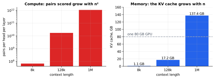
Reading it: the left panel counts query-key pairs per head per layer, on a logarithmic axis where each gridline is ten times the last: every step to the right multiplies the bar by 256 and then by 64. The right panel is the KV cache for one conversation on an ordinary axis, with the dashed line at 80 GB, the memory of one large GPU. The 1M bar crosses it before any weights are loaded. The left panel is the compute bill; the right panel is the memory bill.
Why it matters in practice. The compute bill is paid once per prompt (prefill), and exact tricks such as FlashAttention make it faster without changing it. The memory bill is paid for as long as a conversation is open, and it decides how many users one GPU can serve. That is why most of the techniques below target the cache.
In code: context_cost returns both lines of the bill for any context length, using primer.ml.inference.kv_cache_bytes for the cache.
2. Sliding-window attention: reading through a letterbox
Everyday picture. You read a long scroll through a letterbox slot that shows only the last w words. On your own you would lose the beginning. But suppose a row of readers sits one above the other, each reading the notes of the reader below through a slot of the same width. Each reader passes things along a little further, like a bucket brigade, so a stack of readers can carry a fact much further back than any one slot shows.
Tiny worked example. Eight tokens, window w = 3: each token reads itself and the two tokens before it.
            key:  0 1 2 3 4 5 6 7
query 0           ✓ · · · · · · ·
query 1           ✓ ✓ · · · · · ·
query 2           ✓ ✓ ✓ · · · · ·
query 3           · ✓ ✓ ✓ · · · ·
query 4           · · ✓ ✓ ✓ · · ·
query 5           · · · ✓ ✓ ✓ · ·
query 6           · · · · ✓ ✓ ✓ ·
query 7           · · · · · ✓ ✓ ✓
That is 1 + 2 + 3 × 6 = 21 scores instead of the 36 a full causal mask needs. Now stack three such layers. Token 7 reads token 5 in the top layer; token 5 had read token 3 in the layer below; token 3 had read token 1 in the layer below that. So after three layers, token 1 can influence token 7, six positions back, but token 0 cannot.
flowchart RL
  subgraph L3["layer 3"]
    a7["token 7"]
  end
  subgraph L2["layer 2"]
    b5["token 5"]
  end
  subgraph L1["layer 1"]
    c3["token 3"]
  end
  subgraph IN["input"]
    d1["token 1"]
    d0["token 0: out of reach"]
  end
  a7 -->|"reads 2 back"| b5 -->|"reads 2 back"| c3 -->|"reads 2 back"| d1
Reading it: read right to left, from token 7 at the top layer down to the input. Each arrow is one layer's window: it can reach at most w − 1 = 2 positions back. Three layers chain three arrows, so the furthest input token 7 can hear from is 3 × 2 = 6 positions back, token 1. Token 0 would need a fourth hop. Information still travels far, but only in stages.
Level 3: the formula and its symbols
$$ M_{ij} = \begin{cases} 1 & \text{if } 0 \le i - j < w \ 0 & \text{otherwise} \end{cases} \qquad\qquad \text{reach} = L\,(w - 1) $$
Symbols
| Symbol | Meaning here | In the example |
|---|---|---|
| $M_{ij}$ | the mask: 1 if query $i$ may read key $j$, 0 if not | row 5: keys 3, 4, 5 |
| $i$, $j$ | the query's position and the key's position | $i = 5$ |
| $i - j$ | how far back the key is; negative means the future | 0, 1, 2 allowed |
| $w$ | the window: how many tokens each query reads, itself included | 3 |
| ${$ | "cases": use the line whose condition holds | |
| $L$ | how many windowed layers are stacked | 3 |
| reach | the furthest back an input can influence an output | 6 |
In words: "a query may read a key if the key is not in the future and is fewer than w positions back; stacking L layers lets information travel L times w − 1 positions."
With the numbers: row 5 allows j = 3, 4, 5 (5 − 3 = 2 < 3). Three layers of w = 3 reach 3 × 2 = 6. Mistral 7B uses w = 4,096 over 32 layers: 32 × 4,095 = 131,040 tokens, about 131k, from a window of 4k.
Level 3: in Python
In Python:
n, w = 8, 3
# M_ij for the row of token 5
[int(0 <= 5 - j < w) for j in range(n)]  # → [0, 0, 0, 1, 1, 1, 0, 0]
# pairs scored: row i keeps min(i + 1, w) keys
sum(min(i + 1, w) for i in range(n))  # → 21
# full causal attention, for comparison
n * (n + 1) // 2  # → 36
# reach after L layers
L = 3
L * (w - 1)  # → 6
# Mistral 7B: 32 layers, a 4,096-token window
32 * (4096 - 1)  # → 131040
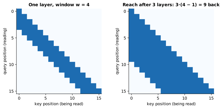
Reading it: both panels are 16 × 16 grids, with rows for the token doing
the looking and columns for the token being looked at, like the causal
heatmap in primer.ml.attention. Dark means "can reach". On the left, one
layer with w = 4 is a thin band along the diagonal: 4 cells per row at most.
On the right, the same mask applied three times: the band has widened to
3 × 3 + 1 = 10 cells, because each layer extends the reach by w − 1 = 3.
Neither panel ever touches the upper-right triangle: the window is still
causal.
In code: sliding_window_mask builds the band, pairs_computed counts its cells, receptive_field applies the mask layer after layer to find who can reach whom, and reach is the L(w − 1) formula.
The rolling buffer: a cache that stops growing
Everyday picture. A whiteboard with room for exactly w notes. When it is full, the next note goes over the oldest one. You never need a bigger board, however long the meeting runs.
Tiny worked example. With w = 4, after token 9 the buffer holds the keys and values of tokens 6, 7, 8 and 9. Token 10 overwrites token 6's slot. On the running 8B example at 128k tokens, a 4,096-token window holds 4,096 × 128 KB = 0.54 GB instead of 17.2 GB: 32 times less, and the same at 1M tokens.
flowchart LR
  subgraph B["buffer of w = 4 slots, after token 9"]
    s0["slot 0: token 8"]
    s1["slot 1: token 9"]
    s2["slot 2: token 6 (oldest)"]
    s3["slot 3: token 7"]
  end
  N["token 10 arrives"] -->|"overwrites the oldest"| s2
  B --> A["token 10 attends to<br/>tokens 7, 8, 9, 10"]
Reading it: the four slots are all the memory there is. Slot number is token number modulo 4 (the remainder after dividing by 4), so token 10 lands in slot 2, where token 6 sat. Token 6 was about to leave the window anyway, so nothing the window needs is lost.
Why it matters in practice. Mistral 7B combined the window with this rolling buffer. Several later model families interleave sliding-window layers with a few full-attention layers: the local layers are cheap, and the full layers keep long-range lookups exact. The weakness is plain from the diagram: a fact beyond the reach is invisible, and a fact inside the reach has to survive several hops.
In code: sliding_window_decode generates token by token with a buffer that never holds more than w keys, and returns the same outputs as masked attention with sliding_window_mask.
3. Sparse attention: a few long-distance lines
Everyday picture. An open-plan office. You mostly talk to the people at the desks next to yours (local). Anyone can phone the front desk, and the front desk hears from everyone (a global token): any two people are at most two calls apart. Another design is the express train: you talk to your neighbours and also to every fourth desk down the row (strided), so a message can travel far in a few big jumps.
Tiny worked example. Sixteen tokens, window 4.
- The window alone: 1 + 2 + 3 + 4 × 13 = 58 pairs.
- Make token 0 global: the 12 rows past the window (tokens 4 to 15) add a pair each: 70 pairs, against 136 for full causal attention.
- Strided with stride 4: the last 4 tokens, plus every 4th token before them. Token 13 reads 10, 11, 12, 13 and then 9, 5, 1. Over all rows that is 58 + 24 = 82 pairs.
flowchart LR
  G(("token 0<br/>global"))
  t3["token 3"] --- G
  t7["token 7"] --- G
  t11["token 11"] --- G
  t15["token 15"] --- G
  t14["token 14"] --- t15
  t13["token 13"] --- t14
Reading it: the circle is the global token. Every token has a line to it, so token 15 can reach token 3 in two hops, through token 0, however long the sequence. The short lines at the bottom are the ordinary local window. The picture is sparse (few lines), yet no two tokens are far apart.
Level 3: the formula and its symbols
$$ M_{ij} = 1 \quad\text{when}\quad i - j \ge 0 \;\text{ and }\; \big(\, i - j < s \;\text{ or }\; (i - j) \bmod s = 0 \,\big) $$
Symbols
| Symbol | Meaning here | In the example |
|---|---|---|
| $M_{ij}$ | 1 if query $i$ may read key $j$ | |
| $i - j$ | how far back key $j$ is | for $i = 13$: 0 to 13 |
| $s$ | the stride: the local width, and the jump between long-range keys | 4 |
| $\bmod$ | "modulo": the remainder after dividing; $(i - j) \bmod s = 0$ means "a whole number of strides back" | 8 mod 4 = 0 |
| and, or | both conditions must hold; at least one must hold |
In words: "never read the future; read the last s tokens, and beyond them every s-th token."
With the numbers: for i = 13, s = 4: distances 0 to 3 give keys 13, 12, 11, 10; distances 4, 8 and 12 give keys 9, 5, 1.
Level 3: in Python
In Python:
s = 4
# row 13: which keys does token 13 read?
[j for j in range(16) if 13 - j >= 0 and (13 - j < s or (13 - j) % s == 0)]  # → [1, 5, 9, 10, 11, 12, 13]
# strided pairs over all 16 rows
sum(1 for i in range(16) for j in range(i + 1) if i - j < s or (i - j) % s == 0)  # → 82
# a window of 4 plus global token 0
sum(1 for i in range(16) for j in range(i + 1) if i - j < 4 or j == 0)  # → 70
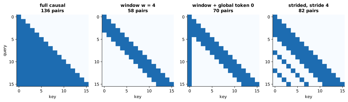
Reading it: each panel is a mask, rows for queries and columns for keys, dark where a score is computed; the title gives the count. The first panel is full causal attention, a solid triangle. The window is a diagonal band. Adding a global token fills in the first column: everyone reads token 0. The strided pattern adds dotted diagonals every 4 columns: the express stops. At 16 tokens the savings look modest; with a fixed window they grow with n, because the band stays w wide while the triangle keeps growing.
Why it matters in practice. The Sparse Transformer introduced strided patterns; Longformer and BigBird combined windows with global tokens (BigBird added a few random links too) to read documents of thousands of tokens. StreamingLLM found that trained models park a lot of attention on the very first tokens (attention sinks); a plain window drops them and falls apart, while keeping the first few tokens plus a window lets a model stream indefinitely. One caution: a sparse pattern only saves time if the GPU kernel skips whole blocks of the score matrix, which is why real patterns are built from blocks.
In code: global_local_mask adds global rows and columns to a window, strided_mask builds the express-stop pattern, and pairs_computed counts what each one scores. Any of them can be passed as the mask to primer.ml.attention.scaled_dot_product_attention, and every skipped pair gets a weight of exactly 0.
4. Linear attention: a pot instead of a guest list
Everyday picture. A potluck soup. In softmax attention every new guest tastes every dish on the table, one by one, and then mixes a bowl: the more dishes, the longer it takes. In linear attention every guest pours their dish into one shared pot as they arrive, and a new guest takes a single ladle, seasoned to their own taste. The pot never grows, and the ladle costs the same for guest 3 as for guest 3 million.
The trick that makes the pot possible: softmax's score $e^{q \cdot k}$ cannot
be split into "a part that depends on q" times "a part that depends on k".
Replace it with $\phi(q) \cdot \phi(k)$, a dot product of transformed
vectors, and it can. Then the order of the matrix multiplies can be swapped:
$(\phi(Q)\phi(K)^\top)\,V = \phi(Q)\,(\phi(K)^\top V)$. The left side builds an
n × n matrix; the right side builds a small d × d one (the pot) and never
builds the big one. Matrix multiplication allows regrouping like this
(associativity), which primer.notation covers under matrix multiply.
Tiny worked example. Three tokens with 2-number keys (1, 0), (0, 1), (1, 1) and one-number values 2, 4, 6. The third token's query is (1, 0). Use the feature map φ(x) = elu(x) + 1, which for a positive number is simply x + 1 and for zero or a negative number is $e^x$ (always above zero).
- φ of the keys: (2, 1), (1, 2), (2, 2).
- Pour into the pot: S = (2, 1)·2 + (1, 2)·4 + (2, 2)·6 = (20, 22), and the running total of keys z = (5, 5).
- Ladle with φ(q) = (2, 1): (2·20 + 1·22) / (2·5 + 1·5) = 62 / 15 = 4.13.
The slow way agrees: the weights φ(q)·φ(k) are 5, 4 and 6, so the output is (5·2 + 4·6 + 6·6) / 15 = 62/15. Softmax attention on the same numbers gives 4.00: linear attention is a different attention, not a faster copy of the same one.
flowchart LR
  subgraph T["each new token i"]
    K["φ(k_i)"]
    V["v_i"]
    Qi["φ(q_i)"]
  end
  K & V -->|"add φ(k_i) v_iᵀ"| S[("pot S<br/>d_k × d_v numbers")]
  K -->|"add φ(k_i)"| Z[("total z<br/>d_k numbers")]
  Qi --> R["output = φ(q_i)ᵀ S / φ(q_i)ᵀ z"]
  S --> R
  Z --> R
Reading it: each token does two things. Its key and value go into the pot S (and its key into the running total z, used to normalize). Its query reads the pot once. S and z have a fixed size set by the head width, not by the number of tokens, so this is a recurrent network: a state updated once per token, with no cache that grows.
Level 3: the formula and its symbols
$$ o_i = \frac{\sum_{j \le i} \big(\phi(q_i) \cdot \phi(k_j)\big)\, v_j}{\sum_{j \le i} \phi(q_i) \cdot \phi(k_j)} = \frac{\phi(q_i)^\top S_i}{\phi(q_i)^\top z_i}, \qquad S_i = S_{i-1} + \phi(k_i)\, v_i^\top, \qquad z_i = z_{i-1} + \phi(k_i) $$
Symbols
| Symbol | Meaning here | In the example |
|---|---|---|
| $o_i$ | the output for token $i$ | $o_3 = 4.13$ |
| $q_i$, $k_j$, $v_j$ | query of token $i$; key and value of token $j$ | $q_3 = (1, 0)$ |
| $\phi$ | the feature map, applied to each number: $x + 1$ if $x > 0$, else $e^x$; always positive so no weight is negative | φ(1, 0) = (2, 1) |
| $\sum_{j \le i}$ | add up over every token $j$ up to and including $i$ (causal) | $j$ = 1, 2, 3 |
| $\phi(q_i) \cdot \phi(k_j)$ | the unnormalized weight, a dot product in place of $e^{q \cdot k}$ | 5, 4, 6 |
| $v_i^\top$ | the value laid on its side as a row | |
| $\phi(k_i)\, v_i^\top$ | an outer product: a column times a row, giving a small table whose entry (m, c) is $\phi(k_i)_m \, v_{i,c}$ | (2, 1) × 2 = (4, 2) |
| $S_i$ | the pot after token $i$: the sum of those tables | (20, 22) |
| $z_i$ | the running sum of $\phi(k_j)$, for the denominator | (5, 5) |
| $\phi(q_i)^\top S_i$ | the query's ladle: its dot product with each column of $S_i$ | 62 |
In words: "each output is a weighted average of the values so far, with weights φ(q)·φ(k); because those weights split into a query part and a key part, the key-and-value part can be kept as a running sum, and each query reads that sum once."
With the numbers: S₃ = (20, 22), z₃ = (5, 5), φ(q₃) = (2, 1): o₃ = (40 + 22) / (10 + 5) = 62/15 = 4.133.
Level 3: in Python
In Python:
import math
def phi(v):
    # elu(x) + 1: x + 1 above zero, e^x at or below it
    return [x + 1 if x > 0 else math.exp(x) for x in v]
def dot(a, b):
    return sum(a_m * b_m for a_m, b_m in zip(a, b))
keys = [[1.0, 0.0], [0.0, 1.0], [1.0, 1.0]]
values = [2.0, 4.0, 6.0]
q3 = [1.0, 0.0]
[phi(k) for k in keys]  # → [[2.0, 1.0], [1.0, 2.0], [2.0, 2.0]]
# S: the running sum of φ(k_j) v_j; z: the running sum of φ(k_j)
S = [sum(phi(k)[m] * v for k, v in zip(keys, values)) for m in range(2)]
S  # → [20.0, 22.0]
z = [sum(phi(k)[m] for k in keys) for m in range(2)]
z  # → [5.0, 5.0]
# o_3 = φ(q)ᵀS / φ(q)ᵀz
round(dot(phi(q3), S) / dot(phi(q3), z), 3)  # → 4.133
# the quadratic form: the weights φ(q)·φ(k_j), then their weighted average
weights = [dot(phi(q3), phi(k)) for k in keys]
weights  # → [5.0, 4.0, 6.0]
round(dot(weights, values) / sum(weights), 3)  # → 4.133
# softmax attention on the same numbers (unscaled), for contrast
e = [math.exp(dot(q3, k)) for k in keys]
round(dot(e, values) / sum(e), 3)  # → 4.0
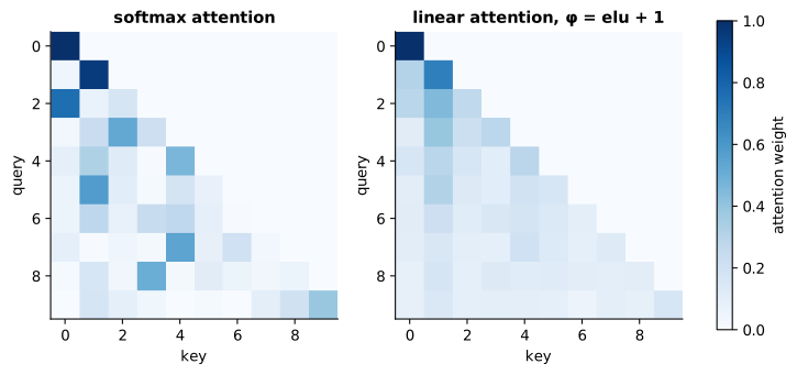
Reading it: the two heatmaps use the same ten queries and keys; rows are
queries, columns are keys, and darker means more weight. Both are causal
triangles and every row sums to 1. On the left, softmax picks favourites:
the exponential stretches gaps between scores (see primer.ml.attention), so
in the last five rows the largest weight averages 0.46. On the right, linear
attention spreads the same rows thinly: its largest weight averages 0.21. The
queries here are twice the usual size, and that is the telling part: at the
usual size the two numbers are 0.28 and 0.20, so making a query more decisive
sharpens softmax a lot and linear attention hardly at all, because φ(q)·φ(k)
never stretches a gap the way $e^x$ does. That bluntness is the price of the
pot: a fixed-size summary cannot pick out one exact token as sharply.
Why it matters in practice. The work drops from n² × d to n × d², and generation needs only the pot, not a cache. The catch is recall: asked to copy back a specific token from far away, a fixed-size pot does worse than a full cache. Later work added forgetting (decay) to the pot, which turns out to be exactly the state-space models of the next section; the Mamba-2 paper shows the two views describe the same computation.
In code: feature_map is φ, linear_attention_quadratic builds all n × n weights (from linear_attention_weights) and blends the values, and linear_attention_recurrent gets the same outputs from the two running sums, returning the fixed-size S and z.
5. State-space models: a summary with a fixed update rule
A recurrence that is also a convolution
Everyday picture. A cup of tea cooling on a desk. Every minute it keeps
some fraction of its heat and gains whatever hot water you pour in. Its
temperature right now is a summary of everything you ever poured, with older
pours counting less. That is a recurrent network's one-page summary (see
primer.ml.cnn_rnn), with one difference: the rewrite rule is linear
(multiply and add, nothing more), and linearity buys a second way to compute
the same thing.
Tiny worked example. The state keeps half of itself each step: A = 0.5, B = 1, C = 1. Inputs x = (1, 0, 0, 2).
| step t | x_t | h_t = 0.5 · h_(t−1) + x_t | y_t |
|---|---|---|---|
| 1 | 1 | 0.5 · 0 + 1 = 1 | 1 |
| 2 | 0 | 0.5 · 1 + 0 = 0.5 | 0.5 |
| 3 | 0 | 0.5 · 0.5 + 0 = 0.25 | 0.25 |
| 4 | 2 | 0.5 · 0.25 + 2 = 2.125 | 2.125 |
Unroll the loop and each output is a weighted sum of all past inputs with weights 1, 0.5, 0.25, 0.125 for "now, 1 step ago, 2 steps ago, 3 steps ago": y₄ = 1·2 + 0.5·0 + 0.25·0 + 0.125·1 = 2.125. The same answer, with no loop.
flowchart LR
  X["inputs x_1 ... x_T"] --> R["recurrence<br/>h_t = A h_(t−1) + B x_t<br/>one step at a time"]
  X --> K["convolution<br/>slide the kernel (CB, CAB, CA²B, ...)<br/>all positions at once"]
  R --> Y["the same outputs y_1 ... y_T"]
  K --> Y
Reading it: two roads from the same inputs to the same outputs. The top
road is how the model generates: one token at a time, carrying a small
state h, with constant memory. The bottom road is how it trains: the
kernel is computed once, and every output is a weighted sum that can be done
in parallel, like a convolution in primer.ml.cnn_rnn. Classic RNNs only had
the top road, which is why they trained slowly.
Level 3: the formula and its symbols
$$ h_t = A\,h_{t-1} + B\,x_t, \qquad y_t = C\,h_t \qquad\Longleftrightarrow\qquad y_t = \sum_{k=0}^{t-1} \big(C A^{k} B\big)\, x_{t-k} $$
Symbols
| Symbol | Meaning here | In the example |
|---|---|---|
| $x_t$ | the input at step $t$ (one channel) | (1, 0, 0, 2) |
| $h_t$ | the state after step $t$: $N$ numbers (here $N$ = 1); $h_0 = 0$ | 1, 0.5, 0.25, 2.125 |
| $A$ | $N \times N$ matrix: how the old state carries over (its size sets how fast things fade) | 0.5 |
| $B$ | how the input is written into the state | 1 |
| $C$ | how the state is read out | 1 |
| $y_t$ | the output at step $t$ | |
| $\Longleftrightarrow$ | "the same thing, written another way" | |
| $A^k$ | $A$ multiplied by itself $k$ times; $A^0$ is "do nothing" | 0.5³ = 0.125 |
| $C A^k B$ | the kernel: how much an input $k$ steps ago still counts now | 1, 0.5, 0.25, 0.125 |
| $\sum_{k=0}^{t-1}$ | add over every look-back distance $k$ from 0 to $t - 1$ |
In words: "the state keeps a fraction of itself and adds the new input, and the output reads the state; equivalently, the output is every past input weighted by how much it has faded since."
With the numbers: y₄ = C A⁰ B x₄ + C A¹ B x₃ + C A² B x₂ + C A³ B x₁ = 1·2 + 0.5·0 + 0.25·0 + 0.125·1 = 2.125.
Level 3: in Python
In Python:
A, B, C = 0.5, 1.0, 1.0
x = [1.0, 0.0, 0.0, 2.0]
h, y = 0.0, []
for x_t in x:
    # keep half of the old state, add the new input
    h = A * h + B * x_t
    y.append(C * h)
y  # → [1.0, 0.5, 0.25, 2.125]
# the kernel C A^k B, for k = 0, 1, 2, 3
kernel = [C * A ** k * B for k in range(4)]
kernel  # → [1.0, 0.5, 0.25, 0.125]
# y_4 as a weighted sum of all four inputs, newest first
sum(kernel[k] * x[3 - k] for k in range(4))  # → 2.125
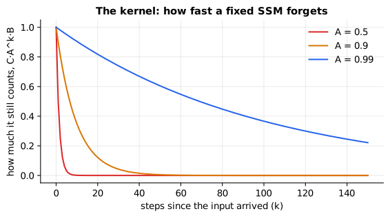
Reading it: the x-axis is how many steps ago an input arrived; the y-axis is how much it still counts (the kernel C A^k B). Each curve is one value of A. With A = 0.5 the curve collapses almost at once: short memory. With A = 0.99 it is still well above zero after 150 steps: long memory. A real SSM layer has thousands of channels, each with its own A, so it remembers at many time scales at once. S4 was the first to make this work on very long sequences, by choosing and computing these kernels carefully.
In code: ssm_recurrent runs the loop, ssm_kernel builds C A^k B, and ssm_convolution gets the same outputs from the kernel with a single NumPy convolution.
Selective: letting each token decide what to keep (Mamba)
Everyday picture. A note-taker with a dial. For filler words ("um", "so", "anyway") they barely touch their notes. For a name or a number they wipe the relevant line and write the new fact. A fixed SSM uses the same dial setting for every word, so it must either write everything (and forget quickly) or write little (and never take in the important word properly). Mamba reads the dial setting off each token itself: that is what selective means.
The dial is a step size Δ. The parameters of the state update are derived from it at every step (this is called discretization: turning a continuous rate of change into one step's keep and write amounts):
- keep factor $\bar{A} = e^{\Delta a}$, with $a$ negative, so a big Δ makes it nearly 0 (forget) and a tiny Δ nearly 1 (keep);
- write factor $\bar{B}$, which goes the opposite way.
Tiny worked example. One channel, a = −1, b = 1. A token that carries a marker gets Δ ≈ 5; an ordinary token gets Δ ≈ 0.0067.
| token | Δ | keep Ā = e^(−Δ) | write B̄ = 1 − e^(−Δ) | effect |
|---|---|---|---|---|
| marked | 5.007 | 0.0067 | 0.9933 | replace the state with this token |
| ordinary | 0.0067 | 0.9933 | 0.0067 | leave the state almost untouched |
The recall task: a sequence of small noise values with one marked 7 in third place, then nine more noise values. The selective SSM writes the 7 almost fully and then keeps it: at the end its state is 6.55. With one fixed Δ for every token, the best any setting manages is 0.26: a Δ big enough to write the 7 also lets the nine later tokens overwrite it.
flowchart LR
  U["token u_t"] --> D["Δ_t = softplus(w · u_t + β)<br/>how much this token matters"]
  D --> AB["Ā_t = e^(Δ_t a): keep<br/>B̄_t: write"]
  U --> XV["x_t: what to write"]
  AB --> H["h_t = Ā_t h_(t−1) + B̄_t x_t"]
  XV --> H
  HP["h_(t−1)"] --> H
  H --> Y["y_t = C h_t"]
Reading it: the new part is the top path. The token itself feeds a small function that produces its step size Δ, which sets how much of the old state to keep and how much of this token to write. In Mamba the matrices B and C are also computed from the token, by the same kind of path. Everything below is the recurrence from before, except that Ā and B̄ now change at every step.
Level 3: the formula and its symbols
$$ \Delta_t = \operatorname{softplus}(w\,u_t + \beta), \qquad \bar{A}_t = e^{\Delta_t a}, \qquad \bar{B}_t = \frac{e^{\Delta_t a} - 1}{a}\, b, \qquad h_t = \bar{A}_t\, h_{t-1} + \bar{B}_t\, x_t $$
Symbols
| Symbol | Meaning here | In the example |
|---|---|---|
| $u_t$ | what the model can see about token $t$ (here, just its marker, 0 or 1) | 1 for the 7 |
| $w$, $\beta$ | learned weight and offset that turn $u_t$ into a step size | 10, −5 |
| softplus | $\log(1 + e^x)$: a smooth ramp that is always positive, about $x$ for large $x$ and about 0 for very negative $x$ | softplus(5) = 5.007 |
| $\Delta_t$ | the step size for token $t$: how much this token matters | 5.007 or 0.0067 |
| $a$ | a negative learned rate; more negative means faster forgetting | −1 |
| $b$ | how strongly inputs are written | 1 |
| $\bar{A}_t$ | this step's keep factor ("A-bar") | 0.0067 or 0.9933 |
| $\bar{B}_t$ | this step's write factor ("B-bar") | 0.9933 or 0.0067 |
| $x_t$, $h_t$ | the value written, and the state after step $t$ | 7, then 6.95 |
In words: "each token computes how much it matters; that sets how much of the old state survives and how much of the token gets written; then the usual update runs with those per-token amounts."
With the numbers: the marked 7 has Δ = softplus(10·1 − 5) = 5.007, so Ā = e^(−5.007) = 0.0067 and B̄ = (0.0067 − 1)/(−1) · 1 = 0.9933: the state becomes about 0.9933 × 7 = 6.95. Each ordinary token after it keeps 0.9933 of the state, and nine of them leave about 6.95 × 0.9933⁹ = 6.55.
Level 3: in Python
In Python:
import math
def softplus(x):
    return math.log(1 + math.exp(x))
a, b = -1.0, 1.0
# Δ for a marked token, then for an ordinary one
d_mark, d_plain = softplus(10 * 1 - 5), softplus(10 * 0 - 5)
round(d_mark, 3), round(d_plain, 4)  # → (5.007, 0.0067)
# Ā_t and B̄_t for the marked token: keep almost nothing, write almost everything
keep_mark, write_mark = math.exp(d_mark * a), (math.exp(d_mark * a) - 1) / a * b
round(keep_mark, 4), round(write_mark, 4)  # → (0.0067, 0.9933)
# and for an ordinary token: keep almost everything, write almost nothing
keep_plain = math.exp(d_plain * a)
round(keep_plain, 4)  # → 0.9933
# the 7 is written once, then kept through nine ordinary tokens
round(write_mark * 7 * keep_plain ** 9, 2)  # → 6.55
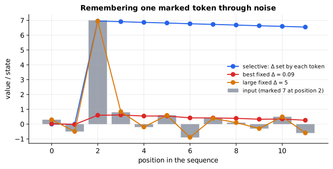
Reading it: the x-axis is the position in the sequence; grey bars are the input values, with the marked 7 at position 2. The blue line is the selective SSM's state: it jumps to the 7 and then barely moves, because every later token has a tiny Δ. The red line is the best fixed Δ: it can only write a small fraction of each input, so the 7 lifts it to about 0.6 at most and it ends at 0.26. The orange line is a large fixed Δ: it writes every token fully, so it tracks whatever arrived last and the 7 is gone by the next step. Only the selective model can both write the important token and ignore the rest.
In code: discretize turns Δ into Ā and B̄, softplus and step_sizes compute each token's Δ, selective_ssm runs the per-token recurrence, and selective_recall and time_invariant_recall run the recall task.
Training in parallel when the kernel keeps changing: the scan
Everyday picture. A relay race where each runner must know the total time so far. Done one after another it takes as long as the whole race. But "multiply by a, then add b" steps can be merged: two consecutive steps are themselves one step of the same shape. So pairs of runners merge their legs, then pairs of pairs, like a knockout tournament: log₂ n rounds instead of n (log₂ n is how many times n can be halved before reaching 1: 10 for 1,024).
Tiny worked example. The four steps of the tea example are (a, b) = (0.5, 1), (0.5, 0), (0.5, 0), (0.5, 2), meaning "h becomes a·h + b". Round 1: every step merges with the one before it. Round 2: every step merges with the result two places before it. After 2 rounds (log₂ 4 = 2), the b parts are 1, 0.5, 0.25, 2.125: every state from the loop.
flowchart TB
  s1["(0.5, 1)"]
  s2["(0.5, 0)"]
  s3["(0.5, 0)"]
  s4["(0.5, 2)"]
  s1 --> r2["(0.25, 0.5)"]
  s2 --> r2
  s2 --> r3["(0.25, 0)"]
  s3 --> r3
  s3 --> r4["(0.25, 2)"]
  s4 --> r4
  s1 --> f3["(0.125, 0.25)"]
  r3 --> f3
  r2 --> f4["(0.0625, 2.125)"]
  r4 --> f4
Reading it: the top row holds the four steps. Each arrow pair is one merge; every merge in a row happens at the same time. The middle row is round 1, the bottom row round 2. Read the second number in each final box (and in s1 and r2, which were already complete): 1, 0.5, 0.25, 2.125, the states from the table above. A selective SSM cannot use the convolution road, because its Ā changes every step, but it can use this one.
Level 3: the formula and its symbols
$$ (a_1, b_1) \circ (a_2, b_2) = \big(a_1 a_2,\; a_2 b_1 + b_2\big) $$
Symbols
| Symbol | Meaning here | In the example |
|---|---|---|
| $(a, b)$ | one step: "multiply the state by $a$, then add $b$" | (0.5, 1) |
| $\circ$ | "do the first step, then the second": merging two steps into one | |
| $a_1 a_2$ | the combined multiplier | 0.25 |
| $a_2 b_1 + b_2$ | the first step's addition, shrunk by the second step, plus the second's own | 0.5·1 + 0 = 0.5 |
In words: "doing step 1 then step 2 is the same as one step that multiplies by both and adds step 1's contribution, faded by step 2."
With the numbers: (0.25, 0.5) ∘ (0.25, 2) = (0.0625, 0.25·0.5 + 2) = (0.0625, 2.125), the last box in the diagram.
Level 3: in Python
In Python:
def merge(first, then):
    a1, b1 = first
    a2, b2 = then
    return (a1 * a2, a2 * b1 + b2)
steps = [(0.5, 1.0), (0.5, 0.0), (0.5, 0.0), (0.5, 2.0)]
# round 1: each step absorbs the one just before it
r1 = [steps[0]] + [merge(steps[t - 1], steps[t]) for t in range(1, 4)]
r1  # → [(0.5, 1.0), (0.25, 0.5), (0.25, 0.0), (0.25, 2.0)]
# round 2: each absorbs the result two places before it
r2 = r1[:2] + [merge(r1[t - 2], r1[t]) for t in range(2, 4)]
[b for a, b in r2]  # → [1.0, 0.5, 0.25, 2.125]
Why it matters in practice. This is how Mamba trains on long sequences at GPU speed despite being recurrent: a parallel scan, written so the state stays in fast on-chip memory. At generation time it switches back to the plain loop, one token at a time, with a state that never grows.
In code: parallel_scan runs the rounds for any length and returns the states and the number of rounds: 10 for 1,024 steps.
Constant memory, and hybrids
Everyday picture. An SSM travels with a backpack of fixed size; the KV cache is a suitcase that grows with every token. A hybrid model mostly uses backpacks but brings one suitcase for every few layers, so it can still look up an exact earlier token when it needs to.
Tiny worked example. One SSM layer with 4,096 channels and a 16-number state per channel holds 4,096 × 16 × 2 bytes = 128 KB, at 10 tokens or at 10 million. One attention layer of the running 8B example holds 537 MB at 128k tokens. Build 32 layers as 4 attention layers and 28 SSM layers (one in eight, the ratio Jamba uses) and the cache at 128k drops from 17.2 GB to 2.15 GB.
flowchart TB
  I["tokens in"] --> M1["SSM layer<br/>fixed state"] --> M2["SSM layer"] --> M3["..."] --> A1["attention layer<br/>KV cache grows"]
  A1 --> M4["SSM layer"] --> M5["..."] --> A2["attention layer"] --> O["next-token scores"]
Reading it: most boxes are SSM layers, each carrying a fixed-size state. Every so often an attention layer sits in the stack; only those keep a KV cache. The memory bill therefore scales with the number of attention layers, not with the total depth, while the attention layers are still there for exact copying and lookup.
Level 3: the formula and its symbols
$$ \text{bytes} = L_{\text{att}} \cdot n \cdot 2\,H_{kv}\,d_h\,b \;+\; (L - L_{\text{att}}) \cdot D \cdot N \cdot b $$
Symbols
| Symbol | Meaning here | In the example |
|---|---|---|
| $L$ | total layers | 32 |
| $L_{\text{att}}$ | how many of them are attention layers | 4 |
| $n$ | context length | 131,072 |
| $2\,H_{kv}\,d_h\,b$ | one attention layer's cache per token (from section 1) | 4,096 bytes |
| $D$ | channels in an SSM layer | 4,096 |
| $N$ | state numbers per channel | 16 |
| $b$ | bytes per number | 2 |
In words: "the attention layers pay per token as before; the SSM layers pay a fixed amount that does not depend on n at all."
With the numbers: 4 × 131,072 × 4,096 = 2,147,483,648 bytes, plus 28 × 4,096 × 16 × 2 = 3,670,016 bytes: 2.15 GB, about one eighth of 17.2 GB.
Level 3: in Python
In Python:
n, H_kv, d_h, b = 131_072, 8, 128, 2
D, N = 4096, 16
# one SSM layer's state, in KB, at any context length
D * N * b / 1024  # → 128.0
# one attention layer's KV cache at 128k tokens, in MB
n * 2 * H_kv * d_h * b / 1e6  # → 536.870912
# 32 layers: all attention, then 4 attention + 28 SSM, in GB
round(32 * n * 2 * H_kv * d_h * b / 1e9, 2)  # → 17.18
round((4 * n * 2 * H_kv * d_h * b + 28 * D * N * b) / 1e9, 2)  # → 2.15
Why it matters in practice. Pure SSMs are strong at language modelling but weaker than attention at copying and exact recall over long contexts, for the same reason as linear attention: a fixed-size state is a summary. Hybrids such as Jamba keep a few attention layers for those jobs and get most of the SSM's memory savings.
In code: ssm_state_bytes is the fixed backpack, and hybrid_cache_bytes adds up a mixed stack.
6. Compressing the KV cache
Fewer key/value heads: GQA and MQA, a recap
Everyday picture. Colleagues sharing one reference binder instead of each keeping a personal copy: everyone still asks their own questions, but the shelf holds fewer binders.
Tiny worked example. On the running example (32 layers, 128 numbers per head, 16-bit), the cache per token for different numbers of KV heads:
| Design | KV heads | Cache per token |
|---|---|---|
| multi-head attention | 32 | 512 KB |
| grouped-query attention | 8 | 128 KB |
| multi-query attention | 1 | 16 KB |
The diagram of shared heads and the full memory arithmetic live in
primer.ml.attention and primer.ml.inference; everything below stacks on
top of whichever of these a model uses.
Latent KV: cache the ingredients, cook on demand
Everyday picture. A restaurant that stores ingredients, not finished dishes. Every head's keys and values can be cooked from a short list of ingredients (the latent vector) with a fixed recipe shared by every token. Store the ingredients, keep the recipe once, and cook when a query needs it. Better still, the recipe can be folded into the query itself, so nothing is ever cooked at all.
Tiny worked example. A token x = (1, 0, 2, 1), two heads of width 2. Ordinary attention would cache 2 heads × 2 numbers × (key and value) = 8 numbers. Instead:
- Squeeze: c = x W_down = (1 + 2, 0 + 1) = (3, 1). Only these 2 numbers are cached: 4 times smaller.
- When needed, expand: k = c W_uk = (3, 1, 3, 1), both heads' keys.
- Or fold the expansion into the query: for q = (1, 2, 0, 1), q · k = 6, and (q W_ukᵀ) · c = (1, 3) · (3, 1) = 6. Same score, and k was never built.
DeepSeek-V2 uses this at scale: its 128 heads of width 128 would cache 32,768 numbers per token per layer; its latent caches 512, plus 64 for a small key that carries position information: 576, about 57 times less.
flowchart LR
  X["token x<br/>(d_model numbers)"] -->|"W_down"| C[("cache: latent c<br/>d_c numbers")]
  C -->|"W_uk"| K["keys for every head"]
  C -->|"W_uv"| V["values for every head"]
  Qn["query q"] -->|"absorbed: q W_ukᵀ"| QL["query in latent space"]
  QL -->|"score directly against c"| C
Reading it: the cylinder is all that is stored per token. The two arrows to the right show the plain way: rebuild keys and values from the latent. The bottom path shows the absorbed way: translate the query into latent space once, then score it against the cached latents directly, and mix latents before expanding with W_uv. Both paths give identical outputs; the absorbed one never materializes the big keys and values.
Level 3: the formula and its symbols
$$ c_t = x_t W^{D}, \qquad k_t = c_t W^{UK}, \qquad v_t = c_t W^{UV}, \qquad q \cdot k_t = \big(q\, {W^{UK}}^{\top}\big) \cdot c_t $$
Symbols
| Symbol | Meaning here | Shape / example |
|---|---|---|
| $x_t$ | token $t$'s vector coming into the layer | $d_\text{model}$; (1, 0, 2, 1) |
| $W^{D}$ | the learned "down" projection that squeezes | $d_\text{model} \times d_c$ |
| $c_t$ | the latent: the only thing cached | $d_c$; (3, 1) |
| $W^{UK}$, $W^{UV}$ | learned "up" projections to every head's keys and values | $d_c \times H d_h$ |
| $k_t$, $v_t$ | token $t$'s keys and values for all heads, side by side | $H d_h$; $k$ = (3, 1, 3, 1) |
| $q$ | a query (one head's slice, or all heads side by side) | (1, 2, 0, 1) |
| ${W^{UK}}^{\top}$ | $W^{UK}$ transposed (rows become columns) | $H d_h \times d_c$ |
| $q\,{W^{UK}}^{\top}$ | the query translated into latent space | $d_c$; (1, 3) |
In words: "squeeze each token into a short latent and cache only that; keys and values are the latent times fixed up-projections, so a query can be moved into latent space once and scored against the cache directly."
With the numbers: c = (3, 1), k = (3, 1, 3, 1), q · k = 3 + 2 + 0 + 1 = 6, and (1, 3) · (3, 1) = 3 + 3 = 6.
Level 3: in Python
In Python:
x = [1, 0, 2, 1]
W_down = [[1, 0], [0, 1], [1, 0], [0, 1]]
W_uk = [[1, 0, 1, 0], [0, 1, 0, 1]]
def vecmat(v, M):
    # row vector times matrix: entry c is Σ_r v_r M[r][c]
    return [sum(v[r] * M[r][c] for r in range(len(v))) for c in range(len(M[0]))]
# c = x W_down: the only thing cached
c = vecmat(x, W_down)
c  # → [3, 1]
# k = c W_uk: both heads' keys, rebuilt on demand
k = vecmat(c, W_uk)
k  # → [3, 1, 3, 1]
q = [1, 2, 0, 1]
sum(q_m * k_m for q_m, k_m in zip(q, k))  # → 6
# absorbed: move q into latent space, then score against c
W_uk_T = [list(col) for col in zip(*W_uk)]
q_latent = vecmat(q, W_uk_T)
q_latent, sum(a * b for a, b in zip(q_latent, c))  # → ([1, 3], 6)
# DeepSeek-V2's shape: cached numbers per token per layer
2 * 128 * 128, 512 + 64, round(2 * 128 * 128 / (512 + 64), 1)  # → (32768, 576, 56.9)
Why can so few numbers stand in for so many? Because every head's keys and
values are built from the same token, they are highly redundant. In the
language of primer.notation, the key projection W^D W^UK has low rank:
however many numbers it outputs, they all vary along only d_c independent
directions. Storing those d_c coordinates loses nothing that projection can
produce. One wrinkle: rotary position embeddings (see primer.ml.positional)
rotate each key by its position, which breaks the absorption trick, so
DeepSeek-V2 carries position in that separate small 64-number key.
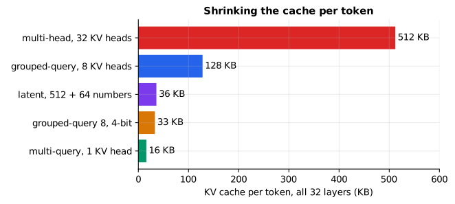
Reading it: each bar is the cache one token costs across all 32 layers of the running example, for one design. The top bar is classic multi-head attention; every bar below it is a way of shrinking it. Sharing heads (GQA, MQA), squeezing into a latent, and cutting bits land in the same range, tens of kilobytes instead of hundreds, by different routes that can be combined.
In code: LatentKVAttention holds the four projections; LatentKVAttention.compress produces the cache, LatentKVAttention.attend expands it into keys and values, and LatentKVAttention.attend_absorbed gets the identical output without expanding. latent_kv_worked_example is the (3, 1) example and latent_kv_bytes_per_token the memory arithmetic.
Quantizing the cache
Everyday picture. The same move as for weights in primer.ml.inference:
write each number to the nearest tenth instead of the nearest thousandth,
with one ruler per stored vector so one big number does not coarsen all the
others.
Tiny worked example. A cached key (0.7, −0.3, 0.2, 0.04) at 4 bits (codes −7 to 7). The step size is 0.7 / 7 = 0.1, the codes are (7, −3, 2, 0), and reading back gives (0.7, −0.3, 0.2, 0): the tiny 0.04 is lost. A 128-number head vector drops from 256 bytes to 64 bytes of codes plus a 2-byte scale: 66 bytes, 3.9 times smaller.
flowchart LR
  KV["new key or value<br/>16-bit numbers"] -->|"scale = max / 7<br/>code = round(x / scale)"| ST[("cache: 4-bit codes<br/>+ one scale per vector")]
  ST -->|"code × scale"| R["approximate key or value"]
  R --> A["attention as usual"]
Reading it: writing to the cache quantizes once per token; reading from it multiplies back. Attention itself is unchanged; it just sees slightly rounded keys and values. The saving is on the cylinder, the part that grows with every token.
Level 3: the formula and its symbols
$$ \text{bytes per token} = 2\,L\,H_{kv}\left(d_h \cdot \frac{\text{bits}}{8} + \frac{\text{scale bits}}{8}\right) $$
Symbols
| Symbol | Meaning here | In the example |
|---|---|---|
| $2\,L\,H_{kv}$ | how many head vectors one token stores: a key and a value per KV head per layer | 2 × 32 × 8 = 512 |
| $d_h$ | numbers per head vector | 128 |
| bits / 8 | bytes per code | 4-bit: 0.5 |
| scale bits / 8 | bytes for the one scale each vector carries | 16-bit: 2 |
In words: "every stored head vector costs its codes plus one scale, and a token stores a key vector and a value vector per head per layer."
With the numbers: 2 × 32 × 8 × (128 × 0.5 + 2) = 512 × 66 = 33,792 bytes, against 131,072 at 16 bits: 3.9 times smaller.
Level 3: in Python
In Python:
k = [0.7, -0.3, 0.2, 0.04]
# one scale per vector: the largest magnitude lands on code 7
s = max(abs(k_j) for k_j in k) / 7
round(s, 3)  # → 0.1
codes = [round(k_j / s) for k_j in k]
codes  # → [7, -3, 2, 0]
[round(s * c, 2) for c in codes]  # → [0.7, -0.3, 0.2, 0.0]
L, H_kv, d_h = 32, 8, 128
# bytes per token: 16-bit, then 4-bit codes plus a 16-bit scale per vector
2 * L * H_kv * d_h * 16 / 8, 2 * L * H_kv * (d_h * 4 / 8 + 16 / 8)  # → (131072.0, 33792.0)
Why it matters in practice. On random test data, an 8-bit cache moves the attention output by under 1% and a 4-bit cache by about 12%; trained models tolerate this far better than random data suggests, and careful schemes go lower. Keys tend to have a few channels with consistently large values, so KIVI quantizes keys per channel and values per token and reaches 2 bits. Quantization stacks with everything above: a GQA model with a sliding window and a 4-bit cache enjoys all three savings.
In code: quantize_kv quantizes each cached vector with its own scale via primer.ml.inference.quantize, quantized_kv_bytes_per_token is the formula, and quantized_cache_error measures how far attention's output moves.
Putting it together
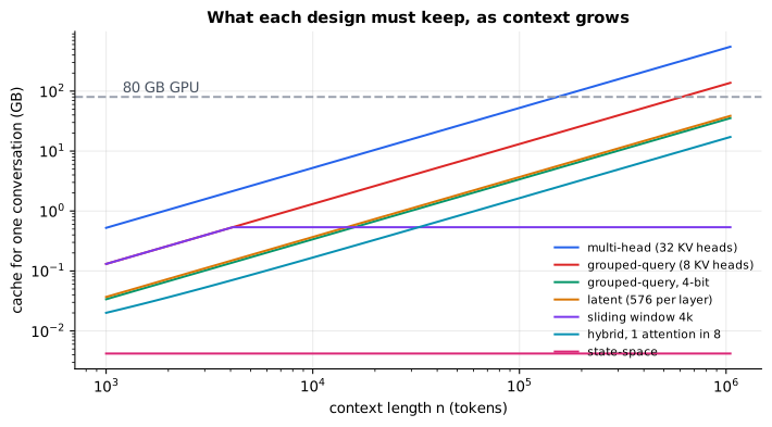
Reading it: the x-axis is context length and the y-axis is cache memory for one conversation, both logarithmic, with the dashed line at 80 GB. Lines with the same slope grow the same way (in proportion to n); compression moves a line down without changing its slope. The sliding window bends flat at 4,096 tokens, and the SSM is flat from the start. Flat lines are what make million-token contexts affordable; the price is that they no longer keep every token exactly.
| Technique | What it cuts | What it gives up |
|---|---|---|
| Sliding window | compute to n·w, cache to w tokens | direct access beyond the window |
| Sparse (global, strided) | compute | exact long-range pairs not in the pattern |
| Linear attention | compute to n·d², cache to a fixed state | sharp, exact recall |
| SSM / Mamba | the same | the same, softened by selectivity |
| Hybrid | most of the cache | a little of both |
| GQA / MQA | cache by the sharing factor | a little modelling capacity |
| Latent KV | cache by d_c / (2·H·d_h) | extra matrix work, care with positions |
| Quantized KV | cache by 16 / bits | a little precision |
In code: cache_bytes_by_method computes every line in the figure for a given context length.
In 20 seconds
- Long context has two bills: attention scores grow with n², and the KV cache grows with n (per layer, per conversation). At 1M tokens the cache of an 8B-class model alone is about 137 GB.
- Sliding window: each token reads the last w; stacked layers still reach L·(w − 1) back, and a rolling buffer caps the cache at w tokens. Sparse patterns add a few global or strided links so any two tokens are a hop or two apart.
- Linear attention replaces e^(q·k) with φ(q)·φ(k), which turns attention into a running sum: O(n) work and a fixed-size state, but blurrier recall.
- State-space models update a fixed state linearly; fixed ones train as a convolution, selective ones (Mamba) let each token set how much to keep and write, and train with a parallel scan. Hybrids keep a few attention layers for exact lookup.
- Compress the cache: share KV heads (GQA/MQA), cache a small latent and expand on demand (latent KV), and store fewer bits per number.
Self-test questions
Why does doubling the context quadruple attention's compute but only double its cache? Every token's query is scored against every key, so the scores form an n × n table: doubling n quadruples it. The cache stores one key and one value per token per layer, a list that grows by one entry per token, so doubling n doubles it.
A model uses a 4,096-token sliding window in all 32 layers. Can token 100,000 be influenced by token 1? Yes, in principle: information moves up to w − 1 = 4,095 positions per layer, so 32 layers reach 131,040 positions back. In practice it must be relayed through about 25 intermediate tokens and layers, so it arrives weakened; direct, exact lookup only works within the window.
What does a global token do in a sparse pattern, and why is it cheap? Every token reads it and it reads every token, so any two tokens are at most two hops apart. It adds only about one column and one row of scores, a cost that grows with n rather than n².
Why can linear attention run as a recurrence but softmax attention cannot? Linear attention's weight φ(q)·φ(k) splits into a query part and a key part, so the key-and-value parts can be summed ahead of time into a fixed-size state that any later query can read. The softmax weight e^(q·k) does not split that way, so each new query must revisit every stored key.
What does "selective" mean in Mamba, and what problem does it fix? The step size Δ, and with it how much of the old state is kept and how much of the new token is written, is computed from each token. A fixed SSM applies the same keep and write amounts to every token, so it cannot both absorb one important token and ignore the filler around it.
If a selective SSM's parameters change every step, how does it train in parallel? The update "multiply by a, add b" can be merged: two consecutive steps form one step of the same kind. A parallel scan merges pairs, then pairs of pairs, and finishes in about log₂ n rounds.
How does latent KV caching save memory without changing the attention outputs? Keys and values are computed as a small cached latent times fixed up-projection matrices, so storing the latent is enough to rebuild them exactly. The up-projection can even be folded into the query and output side, so the full keys and values are never built.
Why do hybrid models keep a few attention layers instead of going all-SSM? A fixed-size state is a lossy summary, which hurts copying and exact recall over long contexts. A handful of attention layers restores exact lookup while most layers keep constant memory, so the cache shrinks roughly by the fraction of layers that are SSMs.
The papers behind this lesson
- Child, Gray, Radford & Sutskever, Generating Long Sequences with Sparse Transformers (2019): https://arxiv.org/abs/1904.10509. Introduced strided and fixed sparse attention patterns, cutting attention's cost to about n√n.
- Beltagy, Peters & Cohan, Longformer: The Long-Document Transformer (2020): https://arxiv.org/abs/2004.05150. Combined a sliding window with task-chosen global tokens to read long documents in linear time.
- Zaheer et al., Big Bird: Transformers for Longer Sequences (2020): https://arxiv.org/abs/2007.14062. Mixed window, global and random links, and proved such sparse attention keeps the expressive power of full attention.
- Katharopoulos et al., Transformers are RNNs: Fast Autoregressive Transformers with Linear Attention (2020): https://arxiv.org/abs/2006.16236. Replaced softmax with a kernel feature map, turning attention into a running sum with O(n) cost.
- Gu, Goel & Ré, Efficiently Modeling Long Sequences with Structured State Spaces (S4, 2021): https://arxiv.org/abs/2111.00396. Made linear state-space layers trainable on very long sequences through the convolution view.
- Gu & Dao, Mamba: Linear-Time Sequence Modeling with Selective State Spaces (2023): https://arxiv.org/abs/2312.00752. Made the state-space parameters depend on the input and trained them with a hardware-aware parallel scan. Annotated companion
- Dao & Gu, Transformers are SSMs (Mamba-2, 2024): https://arxiv.org/abs/2405.21060. Showed that selective SSMs and a form of linear attention are two views of one computation.
- Jiang et al., Mistral 7B (2023): https://arxiv.org/abs/2310.06825. Used sliding-window attention with a rolling-buffer cache in a strong open model. Annotated companion
- Xiao et al., Efficient Streaming Language Models with Attention Sinks (2023): https://arxiv.org/abs/2309.17453. Found that models lean on the first few tokens, and that keeping them plus a window allows streaming without limit.
- Lieber et al., Jamba: A Hybrid Transformer-Mamba Language Model (2024): https://arxiv.org/abs/2403.19887. Interleaved one attention layer per seven Mamba layers to cut the KV cache while keeping recall.
- Shazeer, Fast Transformer Decoding: One Write-Head is All You Need (2019): https://arxiv.org/abs/1911.02150. Introduced multi-query attention, one shared key/value head for all query heads. Annotated companion
- DeepSeek-AI, DeepSeek-V2 (2024): https://arxiv.org/abs/2405.04434. Introduced multi-head latent attention, caching a small latent per token instead of full keys and values.
- Liu et al., KIVI: A Tuning-Free Asymmetric 2bit Quantization for KV Cache (2024): https://arxiv.org/abs/2402.02750. Quantized keys per channel and values per token, bringing the cache down to 2 bits.
Further reading
- Child et al., Sparse Transformers (2019): https://arxiv.org/abs/1904.10509
- Beltagy et al., Longformer (2020): https://arxiv.org/abs/2004.05150
- Katharopoulos et al., Transformers are RNNs (2020): https://arxiv.org/abs/2006.16236
- Gu, Goel & Ré, S4 (2021): https://arxiv.org/abs/2111.00396
- Sasha Rush et al., The Annotated S4 (the S4 paper, line by line in code): https://srush.github.io/annotated-s4/
- Gu & Dao, Mamba (2023): https://arxiv.org/abs/2312.00752
- Dao & Gu, Mamba-2 (2024): https://arxiv.org/abs/2405.21060
- Lieber et al., Jamba (2024): https://arxiv.org/abs/2403.19887
- DeepSeek-AI, DeepSeek-V2 (2024): https://arxiv.org/abs/2405.04434
- Ainslie et al., GQA (2023): https://arxiv.org/abs/2305.13245
1r""" 2# Long context and efficient architectures: reading a million tokens without a million-squared bill 3 4Run: `python -m primer.ml.efficient_architectures` 5 6New to the notation? `primer.notation` explains every symbol used here from 7zero. This lesson builds on attention from `primer.ml.attention` and the KV 8cache from `primer.ml.inference`. 9 10## Level 1: The practitioner's guide 11 12**In one sentence.** Long context is paid for twice, in compute that grows 13with the square of the length and in cache memory that grows with the 14length, and every "efficient" architecture is a different bargain about 15which tokens a model keeps exactly, which it summarizes, and how compactly 16it stores them. 17 18**When you need it.** You need this when a model's context window is part 19of your design: a whole codebase in the prompt, a day-long conversation, a 20document set that will not fit in retrieval, or an agent that runs for 21hundreds of steps. You also need it when choosing between models whose 22cards list different attention designs (grouped-query, sliding-window, 23hybrid Mamba, latent attention), because those words decide what the model 24will cost you per conversation and what it will forget. The tell is a 25context length that sounds like a solved problem. On this lesson's 26Llama-3-8B-shaped model, a 128,000-token conversation holds 17.2 GB of 27cache and a million-token one 137 GB, more than an 80 GB GPU before any 28weights are loaded, and the attention work grows 16,384-fold across that 29same range (this lesson's context-cost table). You do not need this lesson 30for prompts of a few thousand tokens: at that length full attention is 31cheap and exact, and nothing here beats it. 32 33**Your options.** Each is a design you choose by choosing a model, or a 34setting you apply to one, from the most exact to the most compact: 35 36| Option | What it does | What it keeps | What it costs | Where it lives | 37|---|---|---|---|---| 38| Full attention with grouped-query heads | Every token reads every earlier token; several query heads share each key/value head | Exact recall of everything in context | 128 KB per token with 8 KV heads on the 8B example, four times less than 32 heads; still 17 GB at 128k | The model's architecture | 39| Sliding-window and interleaved layers | Each token reads the last w tokens; depth relays information further; some models keep a few full-attention layers | Exact recall inside the window, relayed and weaker beyond it | A cache capped at w tokens: 0.54 GB for a 4,096 window on the 8B example, whatever the length | The model's architecture | 40| Attention sinks with a window | Keeps the first few tokens plus a recent window at serving time | Fluent streaming without limit; no recall of the dropped middle | Nearly nothing; StreamingLLM reports streaming to 4 million tokens and up to 22.2× speedup over recomputation | The inference server | 41| Hybrid state-space and attention | Most layers carry a fixed-size state; one in several is attention | Exact lookup through the attention layers, cheap everything else | On the 8B shape, 4 attention layers in 32 cut the 128k cache from 17.2 GB to 2.15 GB (this lesson's hybrid formula) | The model's architecture | 42| Pure state-space or linear attention | Every layer summarizes the past into a fixed state | Fluent long text; blurrier exact recall | A cache that never grows (4 MB for the whole 8B-shaped stack in this lesson's demo); weaker copying of exact tokens from far back | The model's architecture | 43| Latent KV cache | Caches a short latent per token and rebuilds keys and values from it | Exact outputs, by construction | DeepSeek-V2 caches 576 numbers per token per layer instead of 32,768 (about 57× less) at the price of extra matrix work | The model's architecture | 44| A quantized KV cache | Stores cached keys and values at 8 or 4 bits with one scale per vector | Slightly rounded attention | 3.9× smaller at 4 bits; under 1% output error at 8 bits and about 12% at 4 bits on random data (this lesson's measurement) | The inference server | 45 46**How to choose.** Start from what the task needs to find, not from the 47advertised window. 48 49- Exact lookups across a long input (a function name in a repository, a 50 clause in a contract): keep full attention in enough layers. A 51 grouped-query model, or a hybrid with attention layers, and a budget for 52 the cache. 53- Long, fluent, forward-moving text (a running transcript, a stream) with 54 no need to quote the distant past: a sliding-window or state-space model 55 is far cheaper, and a sink-plus-window server setting keeps even a 56 full-attention model streaming. 57- Many concurrent long conversations on fixed hardware: the cache per 58 token is your capacity. Prefer fewer KV heads or a latent cache, then 59 quantize the cache, then cap the context you allow. 60- A context window claimed at 128k or more: test the model at the length 61 you will use. RULER (Hsieh et al., 2024) found that of 17 models claiming 62 32k tokens or more, only half held up at 32k, and *Lost in the Middle* 63 (Liu et al., 2023) found accuracy highest when the relevant passage sits 64 at the start or the end of the input and worst in the middle. 65- Whatever you pick, put the facts the model must use where the design 66 keeps them exactly: inside the window, near the ends, or in the prompt of 67 a retrieval step (`primer.agents.rag`) instead of a million-token dump. 68 69**What it costs.** Two meters run at once. Compute is the square of the 70length and is paid at prefill: on 4,096 tokens, full attention scores 32 71times as many pairs as a 64-token window (this lesson's demo). Memory is 72linear in the length and is paid for as long as a conversation stays open; 73it decides how many users a GPU serves. The compressions differ in what 74they charge: grouped-query heads cost a little modelling capacity; the 75window costs direct access beyond it; a fixed state costs sharp recall 76(in this lesson's comparison, softmax attention puts up to 0.46 of a row 77on its favourite key where linear attention manages 0.21); the latent 78cache costs extra matrix work and care with positions; quantization costs 79precision. The gains are large: Mamba reports 5× the inference throughput 80of a transformer with linear scaling in length, DeepSeek-V2 reports a KV 81cache 93.3% smaller and 5.76× the generation throughput of its 82predecessor, and Jamba fits a 256k-context model on one 80 GB GPU (each 83paper's abstract). 84 85**What breaks.** 86 87- **The fact was outside the window.** A sliding-window model can be 88 influenced by a token 131,040 positions back (Mistral 7B's 32 layers of 89 4,096), but only by relay through about 25 hops, so a distant fact 90 arrives weakened. Do not expect exact quotes from beyond the window. 91- **A plain window drops the first tokens and the model falls apart.** 92 Trained models park attention on the first few tokens (attention sinks); 93 keep them when you truncate. 94- **A fixed-size state cannot copy.** Pure state-space and linear-attention 95 models do worse at reproducing a specific token from far back. If the 96 task is retrieval or copying, keep attention layers. 97- **The advertised context is not the effective context.** Test at your 98 length with your task, in the middle of the input, not only with a 99 needle at the end. 100- **A sparse pattern that saves no time.** Skipped pairs only save work 101 when the kernel skips whole blocks of the score matrix; a pattern drawn 102 token by token costs as much as full attention. 103- **A quantized cache that changes answers.** Keys carry a few channels 104 with large values; quantizing per token can lose them. Check outputs on 105 your own data, and use a scheme like KIVI's (keys per channel, values 106 per token) at low bit widths. 107 108**In the wild.** Mistral 7B (Jiang et al.) shipped sliding-window attention 109with a rolling-buffer cache; Llama 3 uses grouped-query attention, the 110design this lesson's 8 KV heads mirror (Grattafiori et al., in 111`primer.ml.inference`). Jamba (Lieber et al.) interleaves one attention 112layer among Mamba layers; Mamba itself (Gu and Dao) and Mamba-2 (Dao and 113Gu) are the state-space models; the Sparse Transformer (Child et al.), 114Longformer (Beltagy et al.) and BigBird (Zaheer et al.) are the sparse 115patterns; StreamingLLM (Xiao et al.) is the sink-plus-window trick; 116DeepSeek-V2 introduced the latent cache; KIVI (Liu et al.) reaches a 2-bit 117cache. RULER and *Lost in the Middle* are the two tests to run before 118trusting a context length. Inference servers expose the serving-side 119options: vLLM and SGLang list quantization and prefix caching among their 120features, and the paged KV memory both use is what makes a growing cache 121manageable at all (`primer.ml.inference`). 122 123**Go deeper.** Level 2 builds every row of the table from nothing: the two 124bills counted for real context lengths, the window mask and the reach it 125gives a stack of layers, sparse patterns with their pair counts, linear 126attention as a running sum, a state-space model that is both a loop and a 127convolution, Mamba's per-token step size on a recall task, the parallel 128scan that trains it, the latent cache with its absorbed query, and a 129quantized cache with its error measured. If you only needed to pick a 130model and size its cache, you are done. 131 132## Level 2: How it works, from scratch 133 134Attention (see `primer.ml.attention`) lets every token look at every earlier 135token. That is where its power comes from, and it is also where its bill comes 136from. The bill has two lines: 137 138- **Compute.** Every token is scored against every other token, so the work 139 grows with the *square* of the context length n. 140- **Memory.** During generation the model keeps every earlier token's keys 141 and values (the KV cache, see `primer.ml.inference`), so memory grows with 142 n, per layer, per conversation. 143 144Everything in this lesson attacks one of those two lines, in one of three ways: 145 1461. **Look at fewer tokens**: sliding-window and sparse attention. 1472. **Summarize the past into a fixed-size state**: linear attention and 148 state-space models (Mamba), which run like a recurrent network. 1493. **Store the past more compactly**: fewer key/value heads, a small latent 150 vector per token, fewer bits per number. 151 152```mermaid 153flowchart TB 154 P["Long context is expensive<br/>compute grows with n², memory with n"] --> F["Look at fewer tokens"] 155 P --> S["Keep a fixed-size summary"] 156 P --> C["Store the past compactly"] 157 F --> F1["sliding window"] & F2["sparse: local + global, strided"] 158 S --> S1["linear attention"] & S2["state-space models, Mamba"] 159 C --> C1["GQA / MQA"] & C2["latent KV"] & C3["quantized KV"] 160 S2 --> H["hybrids: a few attention layers<br/>among many SSM layers"] 161 F1 --> H 162``` 163 164**Reading it:** start at the top box, the problem. The three arrows below it 165are the three strategies, and the leaves are the techniques this lesson 166builds from scratch, section by section. The bottom box is where real 167models often land: a mix, keeping a little full attention for exact lookups 168and using cheap layers for everything else. 169 170## 1. Why long context is expensive 171 172**Everyday picture.** A dinner party where every new guest must shake hands 173with every guest already there. Ten guests make 45 handshakes; a thousand 174guests make half a million. On top of that, the coat check keeps one coat per 175guest on every floor of the building, so the coat racks grow with every 176arrival. Attention pays both bills: the handshakes are the query-key scores, 177and the coats are the KV cache. 178 179**Tiny worked example.** Take a Llama-3-8B-shaped model: 32 layers, 8 180key/value heads, 128 numbers per head, 16-bit numbers (2 bytes). One token 181costs 2 × 32 × 8 × 128 × 2 = 131,072 bytes of cache, about 128 KB. 182 183| Context n | Pairs scored per head per layer (n²) | KV cache for one conversation | 184|---|---|---| 185| 8,192 (8k) | 67 million | 1.1 GB | 186| 131,072 (128k) | 17 billion | 17.2 GB | 187| 1,048,576 (1M) | 1.1 trillion | 137.4 GB | 188 189Going from 8k to 1M is 128 times more tokens, 16,384 times more pairs, and a 190cache that no longer fits on one 80 GB GPU. 191 192```mermaid 193flowchart LR 194 T["new token n"] --> Q["its query"] 195 Q -->|"scored against"| KC[("KV cache<br/>n − 1 keys and values<br/>per layer")] 196 KC --> O["output for token n"] 197 T -->|"its key and value<br/>are appended"| KC 198``` 199 200**Reading it:** follow one new token. Its query is scored against every key 201already in the cache, so the work for this one token grows with n, and the 202work for all n tokens grows with n². Then its own key and value are appended, 203so the cache grows by one entry, in every layer, for every token. The two 204arrows into the cache are the two bills. 205 206$$ 207\text{pairs} = n^2 \qquad\qquad \text{KV bytes} = 2 \, L \, H_{kv} \, d_h \, b \, n 208$$ 209 210**Symbols** 211 212| Symbol | Meaning here | In the example | 213|---|---|---| 214| $n$ | context length: how many tokens are in play | 131,072 | 215| $n^2$ | $n$ times $n$: every query paired with every key (causal masking halves it, which does not change how it grows) | 17,179,869,184 | 216| $2$ | one key and one value per token | | 217| $L$ | layers, each with its own cache | 32 | 218| $H_{kv}$ | key/value heads per layer | 8 | 219| $d_h$ | numbers per head | 128 | 220| $b$ | bytes per stored number | 2 (16-bit) | 221 222**In words:** "the score work is the context length squared, and the cache 223holds a key and a value for every head, in every layer, for every token." 224 225**With the numbers:** at n = 131,072 the pairs are 131,072² ≈ 1.7 × 10¹⁰, 226and the cache is 2 × 32 × 8 × 128 × 2 × 131,072 = 17,179,869,184 bytes ≈ 22717.2 GB. 228 229**In Python:** 230 231```python 232L, H_kv, d_h, b = 32, 8, 128, 2 233# bytes per token: a key and a value, per layer, per KV head 234per_token = 2 * L * H_kv * d_h * b 235per_token # → 131072 236contexts = [8_192, 131_072, 1_048_576] 237# pairs per head per layer 238[f"{n * n:,}" for n in contexts] # → ['67,108,864', '17,179,869,184', '1,099,511,627,776'] 239# GB of cache for one conversation 240[round(n * per_token / 1e9, 1) for n in contexts] # → [1.1, 17.2, 137.4] 241``` 242 243 244 245**Reading it:** the left panel counts query-key pairs per head per layer, on 246a logarithmic axis where each gridline is ten times the last: every step to 247the right multiplies the bar by 256 and then by 64. The right panel is the KV 248cache for one conversation on an ordinary axis, with the dashed line at 80 GB, 249the memory of one large GPU. The 1M bar crosses it before any weights are 250loaded. The left panel is the compute bill; the right panel is the memory 251bill. 252 253**Why it matters in practice.** The compute bill is paid once per prompt 254(prefill), and exact tricks such as FlashAttention make it faster without 255changing it. The memory bill is paid for as long as a conversation is open, 256and it decides how many users one GPU can serve. That is why most of the 257techniques below target the cache. 258 259**In code:** `context_cost` returns both lines of the bill for any context length, using `primer.ml.inference.kv_cache_bytes` for the cache. 260 261## 2. Sliding-window attention: reading through a letterbox 262 263**Everyday picture.** You read a long scroll through a letterbox slot that 264shows only the last w words. On your own you would lose the beginning. But 265suppose a row of readers sits one above the other, each reading the notes of 266the reader below through a slot of the same width. Each reader passes things 267along a little further, like a bucket brigade, so a stack of readers can 268carry a fact much further back than any one slot shows. 269 270**Tiny worked example.** Eight tokens, window w = 3: each token reads itself 271and the two tokens before it. 272 273```text 274 key: 0 1 2 3 4 5 6 7 275query 0 ✓ · · · · · · · 276query 1 ✓ ✓ · · · · · · 277query 2 ✓ ✓ ✓ · · · · · 278query 3 · ✓ ✓ ✓ · · · · 279query 4 · · ✓ ✓ ✓ · · · 280query 5 · · · ✓ ✓ ✓ · · 281query 6 · · · · ✓ ✓ ✓ · 282query 7 · · · · · ✓ ✓ ✓ 283``` 284 285That is 1 + 2 + 3 × 6 = **21** scores instead of the 36 a full causal mask 286needs. Now stack three such layers. Token 7 reads token 5 in the top layer; 287token 5 had read token 3 in the layer below; token 3 had read token 1 in the 288layer below that. So after three layers, token 1 can influence token 7, six 289positions back, but token 0 cannot. 290 291```mermaid 292flowchart RL 293 subgraph L3["layer 3"] 294 a7["token 7"] 295 end 296 subgraph L2["layer 2"] 297 b5["token 5"] 298 end 299 subgraph L1["layer 1"] 300 c3["token 3"] 301 end 302 subgraph IN["input"] 303 d1["token 1"] 304 d0["token 0: out of reach"] 305 end 306 a7 -->|"reads 2 back"| b5 -->|"reads 2 back"| c3 -->|"reads 2 back"| d1 307``` 308 309**Reading it:** read right to left, from token 7 at the top layer down to the 310input. Each arrow is one layer's window: it can reach at most w − 1 = 2 311positions back. Three layers chain three arrows, so the furthest input token 7 312can hear from is 3 × 2 = 6 positions back, token 1. Token 0 would need a 313fourth hop. Information still travels far, but only in stages. 314 315$$ 316M_{ij} = \begin{cases} 1 & \text{if } 0 \le i - j < w \\ 0 & \text{otherwise} \end{cases} 317\qquad\qquad 318\text{reach} = L\,(w - 1) 319$$ 320 321**Symbols** 322 323| Symbol | Meaning here | In the example | 324|---|---|---| 325| $M_{ij}$ | the mask: 1 if query $i$ may read key $j$, 0 if not | row 5: keys 3, 4, 5 | 326| $i$, $j$ | the query's position and the key's position | $i = 5$ | 327| $i - j$ | how far back the key is; negative means the future | 0, 1, 2 allowed | 328| $w$ | the window: how many tokens each query reads, itself included | 3 | 329| $\{$ | "cases": use the line whose condition holds | | 330| $L$ | how many windowed layers are stacked | 3 | 331| reach | the furthest back an input can influence an output | 6 | 332 333**In words:** "a query may read a key if the key is not in the future and is 334fewer than w positions back; stacking L layers lets information travel 335L times w − 1 positions." 336 337**With the numbers:** row 5 allows j = 3, 4, 5 (5 − 3 = 2 < 3). Three layers 338of w = 3 reach 3 × 2 = 6. Mistral 7B uses w = 4,096 over 32 layers: 33932 × 4,095 = 131,040 tokens, about 131k, from a window of 4k. 340 341**In Python:** 342 343```python 344n, w = 8, 3 345# M_ij for the row of token 5 346[int(0 <= 5 - j < w) for j in range(n)] # → [0, 0, 0, 1, 1, 1, 0, 0] 347# pairs scored: row i keeps min(i + 1, w) keys 348sum(min(i + 1, w) for i in range(n)) # → 21 349# full causal attention, for comparison 350n * (n + 1) // 2 # → 36 351# reach after L layers 352L = 3 353L * (w - 1) # → 6 354# Mistral 7B: 32 layers, a 4,096-token window 35532 * (4096 - 1) # → 131040 356``` 357 358 359 360**Reading it:** both panels are 16 × 16 grids, with rows for the token doing 361the looking and columns for the token being looked at, like the causal 362heatmap in `primer.ml.attention`. Dark means "can reach". On the left, one 363layer with w = 4 is a thin band along the diagonal: 4 cells per row at most. 364On the right, the same mask applied three times: the band has widened to 3653 × 3 + 1 = 10 cells, because each layer extends the reach by w − 1 = 3. 366Neither panel ever touches the upper-right triangle: the window is still 367causal. 368 369**In code:** `sliding_window_mask` builds the band, `pairs_computed` counts its cells, `receptive_field` applies the mask layer after layer to find who can reach whom, and `reach` is the L(w − 1) formula. 370 371### The rolling buffer: a cache that stops growing 372 373**Everyday picture.** A whiteboard with room for exactly w notes. When it is 374full, the next note goes over the oldest one. You never need a bigger board, 375however long the meeting runs. 376 377**Tiny worked example.** With w = 4, after token 9 the buffer holds the keys 378and values of tokens 6, 7, 8 and 9. Token 10 overwrites token 6's slot. On 379the running 8B example at 128k tokens, a 4,096-token window holds 4,096 × 128 380KB = 0.54 GB instead of 17.2 GB: **32 times less**, and the same at 1M tokens. 381 382```mermaid 383flowchart LR 384 subgraph B["buffer of w = 4 slots, after token 9"] 385 s0["slot 0: token 8"] 386 s1["slot 1: token 9"] 387 s2["slot 2: token 6 (oldest)"] 388 s3["slot 3: token 7"] 389 end 390 N["token 10 arrives"] -->|"overwrites the oldest"| s2 391 B --> A["token 10 attends to<br/>tokens 7, 8, 9, 10"] 392``` 393 394**Reading it:** the four slots are all the memory there is. Slot number is 395token number modulo 4 (the remainder after dividing by 4), so token 10 lands 396in slot 2, where token 6 sat. Token 6 was about to leave the window anyway, 397so nothing the window needs is lost. 398 399**Why it matters in practice.** Mistral 7B combined the window with this 400rolling buffer. Several later model families interleave sliding-window layers 401with a few full-attention layers: the local layers are cheap, and the full 402layers keep long-range lookups exact. The weakness is plain from the diagram: 403a fact beyond the reach is invisible, and a fact inside the reach has to 404survive several hops. 405 406**In code:** `sliding_window_decode` generates token by token with a buffer that never holds more than w keys, and returns the same outputs as masked attention with `sliding_window_mask`. 407 408## 3. Sparse attention: a few long-distance lines 409 410**Everyday picture.** An open-plan office. You mostly talk to the people at 411the desks next to yours (local). Anyone can phone the front desk, and the 412front desk hears from everyone (a *global* token): any two people are at 413most two calls apart. Another design is the express train: you talk to your 414neighbours and also to every fourth desk down the row (*strided*), so a 415message can travel far in a few big jumps. 416 417**Tiny worked example.** Sixteen tokens, window 4. 418 419- The window alone: 1 + 2 + 3 + 4 × 13 = **58** pairs. 420- Make token 0 global: the 12 rows past the window (tokens 4 to 15) add a 421 pair each: **70** pairs, against **136** for full causal attention. 422- Strided with stride 4: the last 4 tokens, plus every 4th token before them. 423 Token 13 reads 10, 11, 12, 13 and then 9, 5, 1. Over all rows that is 424 58 + 24 = **82** pairs. 425 426```mermaid 427flowchart LR 428 G(("token 0<br/>global")) 429 t3["token 3"] --- G 430 t7["token 7"] --- G 431 t11["token 11"] --- G 432 t15["token 15"] --- G 433 t14["token 14"] --- t15 434 t13["token 13"] --- t14 435``` 436 437**Reading it:** the circle is the global token. Every token has a line to 438it, so token 15 can reach token 3 in two hops, through token 0, however long 439the sequence. The short lines at the bottom are the ordinary local window. 440The picture is sparse (few lines), yet no two tokens are far apart. 441 442$$ 443M_{ij} = 1 \quad\text{when}\quad i - j \ge 0 \;\text{ and }\; \big(\, i - j < s \;\text{ or }\; (i - j) \bmod s = 0 \,\big) 444$$ 445 446**Symbols** 447 448| Symbol | Meaning here | In the example | 449|---|---|---| 450| $M_{ij}$ | 1 if query $i$ may read key $j$ | | 451| $i - j$ | how far back key $j$ is | for $i = 13$: 0 to 13 | 452| $s$ | the stride: the local width, and the jump between long-range keys | 4 | 453| $\bmod$ | "modulo": the remainder after dividing; $(i - j) \bmod s = 0$ means "a whole number of strides back" | 8 mod 4 = 0 | 454| and, or | both conditions must hold; at least one must hold | | 455 456**In words:** "never read the future; read the last s tokens, and beyond 457them every s-th token." 458 459**With the numbers:** for i = 13, s = 4: distances 0 to 3 give keys 13, 12, 46011, 10; distances 4, 8 and 12 give keys 9, 5, 1. 461 462**In Python:** 463 464```python 465s = 4 466# row 13: which keys does token 13 read? 467[j for j in range(16) if 13 - j >= 0 and (13 - j < s or (13 - j) % s == 0)] # → [1, 5, 9, 10, 11, 12, 13] 468# strided pairs over all 16 rows 469sum(1 for i in range(16) for j in range(i + 1) if i - j < s or (i - j) % s == 0) # → 82 470# a window of 4 plus global token 0 471sum(1 for i in range(16) for j in range(i + 1) if i - j < 4 or j == 0) # → 70 472``` 473 474 475 476**Reading it:** each panel is a mask, rows for queries and columns for keys, 477dark where a score is computed; the title gives the count. The first panel 478is full causal attention, a solid triangle. The window is a diagonal band. 479Adding a global token fills in the first column: everyone reads token 0. The 480strided pattern adds dotted diagonals every 4 columns: the express stops. At 48116 tokens the savings look modest; with a fixed window they grow with n, 482because the band stays w wide while the triangle keeps growing. 483 484**Why it matters in practice.** The Sparse Transformer introduced strided 485patterns; Longformer and BigBird combined windows with global tokens (BigBird 486added a few random links too) to read documents of thousands of tokens. 487StreamingLLM found that trained models park a lot of attention on the very 488first tokens (*attention sinks*); a plain window drops them and falls apart, 489while keeping the first few tokens plus a window lets a model stream 490indefinitely. One caution: a sparse pattern only saves time if the GPU 491kernel skips whole blocks of the score matrix, which is why real patterns 492are built from blocks. 493 494**In code:** `global_local_mask` adds global rows and columns to a window, `strided_mask` builds the express-stop pattern, and `pairs_computed` counts what each one scores. Any of them can be passed as the mask to `primer.ml.attention.scaled_dot_product_attention`, and every skipped pair gets a weight of exactly 0. 495 496## 4. Linear attention: a pot instead of a guest list 497 498**Everyday picture.** A potluck soup. In softmax attention every new guest 499tastes every dish on the table, one by one, and then mixes a bowl: the more 500dishes, the longer it takes. In linear attention every guest pours their dish 501into one shared pot as they arrive, and a new guest takes a single ladle, 502seasoned to their own taste. The pot never grows, and the ladle costs the 503same for guest 3 as for guest 3 million. 504 505The trick that makes the pot possible: softmax's score $e^{q \cdot k}$ cannot 506be split into "a part that depends on q" times "a part that depends on k". 507Replace it with $\phi(q) \cdot \phi(k)$, a dot product of transformed 508vectors, and it can. Then the order of the matrix multiplies can be swapped: 509$(\phi(Q)\phi(K)^\top)\,V = \phi(Q)\,(\phi(K)^\top V)$. The left side builds an 510n × n matrix; the right side builds a small d × d one (the pot) and never 511builds the big one. Matrix multiplication allows regrouping like this 512(*associativity*), which `primer.notation` covers under matrix multiply. 513 514**Tiny worked example.** Three tokens with 2-number keys (1, 0), (0, 1), 515(1, 1) and one-number values 2, 4, 6. The third token's query is (1, 0). Use 516the feature map φ(x) = elu(x) + 1, which for a positive number is simply 517x + 1 and for zero or a negative number is $e^x$ (always above zero). 518 5191. φ of the keys: (2, 1), (1, 2), (2, 2). 5202. Pour into the pot: S = (2, 1)·2 + (1, 2)·4 + (2, 2)·6 = (20, 22), and the 521 running total of keys z = (5, 5). 5223. Ladle with φ(q) = (2, 1): (2·20 + 1·22) / (2·5 + 1·5) = 62 / 15 = **4.13**. 523 524The slow way agrees: the weights φ(q)·φ(k) are 5, 4 and 6, so the output is 525(5·2 + 4·6 + 6·6) / 15 = 62/15. Softmax attention on the same numbers gives 526**4.00**: linear attention is a *different* attention, not a faster copy of 527the same one. 528 529```mermaid 530flowchart LR 531 subgraph T["each new token i"] 532 K["φ(k_i)"] 533 V["v_i"] 534 Qi["φ(q_i)"] 535 end 536 K & V -->|"add φ(k_i) v_iᵀ"| S[("pot S<br/>d_k × d_v numbers")] 537 K -->|"add φ(k_i)"| Z[("total z<br/>d_k numbers")] 538 Qi --> R["output = φ(q_i)ᵀ S / φ(q_i)ᵀ z"] 539 S --> R 540 Z --> R 541``` 542 543**Reading it:** each token does two things. Its key and value go into the 544pot S (and its key into the running total z, used to normalize). Its query 545reads the pot once. S and z have a fixed size set by the head width, not by 546the number of tokens, so this is a recurrent network: a state updated once 547per token, with no cache that grows. 548 549$$ 550o_i = \frac{\sum_{j \le i} \big(\phi(q_i) \cdot \phi(k_j)\big)\, v_j}{\sum_{j \le i} \phi(q_i) \cdot \phi(k_j)} 551= \frac{\phi(q_i)^\top S_i}{\phi(q_i)^\top z_i}, 552\qquad S_i = S_{i-1} + \phi(k_i)\, v_i^\top, 553\qquad z_i = z_{i-1} + \phi(k_i) 554$$ 555 556**Symbols** 557 558| Symbol | Meaning here | In the example | 559|---|---|---| 560| $o_i$ | the output for token $i$ | $o_3 = 4.13$ | 561| $q_i$, $k_j$, $v_j$ | query of token $i$; key and value of token $j$ | $q_3 = (1, 0)$ | 562| $\phi$ | the feature map, applied to each number: $x + 1$ if $x > 0$, else $e^x$; always positive so no weight is negative | φ(1, 0) = (2, 1) | 563| $\sum_{j \le i}$ | add up over every token $j$ up to and including $i$ (causal) | $j$ = 1, 2, 3 | 564| $\phi(q_i) \cdot \phi(k_j)$ | the unnormalized weight, a dot product in place of $e^{q \cdot k}$ | 5, 4, 6 | 565| $v_i^\top$ | the value laid on its side as a row | | 566| $\phi(k_i)\, v_i^\top$ | an **outer product**: a column times a row, giving a small table whose entry (m, c) is $\phi(k_i)_m \, v_{i,c}$ | (2, 1) × 2 = (4, 2) | 567| $S_i$ | the pot after token $i$: the sum of those tables | (20, 22) | 568| $z_i$ | the running sum of $\phi(k_j)$, for the denominator | (5, 5) | 569| $\phi(q_i)^\top S_i$ | the query's ladle: its dot product with each column of $S_i$ | 62 | 570 571**In words:** "each output is a weighted average of the values so far, with 572weights φ(q)·φ(k); because those weights split into a query part and a key 573part, the key-and-value part can be kept as a running sum, and each query 574reads that sum once." 575 576**With the numbers:** S₃ = (20, 22), z₃ = (5, 5), φ(q₃) = (2, 1): 577o₃ = (40 + 22) / (10 + 5) = 62/15 = 4.133. 578 579**In Python:** 580 581```python 582import math 583def phi(v): 584 # elu(x) + 1: x + 1 above zero, e^x at or below it 585 return [x + 1 if x > 0 else math.exp(x) for x in v] 586def dot(a, b): 587 return sum(a_m * b_m for a_m, b_m in zip(a, b)) 588keys = [[1.0, 0.0], [0.0, 1.0], [1.0, 1.0]] 589values = [2.0, 4.0, 6.0] 590q3 = [1.0, 0.0] 591[phi(k) for k in keys] # → [[2.0, 1.0], [1.0, 2.0], [2.0, 2.0]] 592# S: the running sum of φ(k_j) v_j; z: the running sum of φ(k_j) 593S = [sum(phi(k)[m] * v for k, v in zip(keys, values)) for m in range(2)] 594S # → [20.0, 22.0] 595z = [sum(phi(k)[m] for k in keys) for m in range(2)] 596z # → [5.0, 5.0] 597# o_3 = φ(q)ᵀS / φ(q)ᵀz 598round(dot(phi(q3), S) / dot(phi(q3), z), 3) # → 4.133 599# the quadratic form: the weights φ(q)·φ(k_j), then their weighted average 600weights = [dot(phi(q3), phi(k)) for k in keys] 601weights # → [5.0, 4.0, 6.0] 602round(dot(weights, values) / sum(weights), 3) # → 4.133 603# softmax attention on the same numbers (unscaled), for contrast 604e = [math.exp(dot(q3, k)) for k in keys] 605round(dot(e, values) / sum(e), 3) # → 4.0 606``` 607 608 609 610**Reading it:** the two heatmaps use the same ten queries and keys; rows are 611queries, columns are keys, and darker means more weight. Both are causal 612triangles and every row sums to 1. On the left, softmax picks favourites: 613the exponential stretches gaps between scores (see `primer.ml.attention`), so 614in the last five rows the largest weight averages 0.46. On the right, linear 615attention spreads the same rows thinly: its largest weight averages 0.21. The 616queries here are twice the usual size, and that is the telling part: at the 617usual size the two numbers are 0.28 and 0.20, so making a query more decisive 618sharpens softmax a lot and linear attention hardly at all, because φ(q)·φ(k) 619never stretches a gap the way $e^x$ does. That bluntness is the price of the 620pot: a fixed-size summary cannot pick out one exact token as sharply. 621 622**Why it matters in practice.** The work drops from n² × d to n × d², and 623generation needs only the pot, not a cache. The catch is recall: asked to 624copy back a specific token from far away, a fixed-size pot does worse than a 625full cache. Later work added forgetting (decay) to the pot, which turns out 626to be exactly the state-space models of the next section; the Mamba-2 paper 627shows the two views describe the same computation. 628 629**In code:** `feature_map` is φ, `linear_attention_quadratic` builds all n × n weights (from `linear_attention_weights`) and blends the values, and `linear_attention_recurrent` gets the same outputs from the two running sums, returning the fixed-size S and z. 630 631## 5. State-space models: a summary with a fixed update rule 632 633### A recurrence that is also a convolution 634 635**Everyday picture.** A cup of tea cooling on a desk. Every minute it keeps 636some fraction of its heat and gains whatever hot water you pour in. Its 637temperature right now is a summary of everything you ever poured, with older 638pours counting less. That is a recurrent network's one-page summary (see 639`primer.ml.cnn_rnn`), with one difference: the rewrite rule is *linear* 640(multiply and add, nothing more), and linearity buys a second way to compute 641the same thing. 642 643**Tiny worked example.** The state keeps half of itself each step: A = 0.5, 644B = 1, C = 1. Inputs x = (1, 0, 0, 2). 645 646| step t | x_t | h_t = 0.5 · h_(t−1) + x_t | y_t | 647|---|---|---|---| 648| 1 | 1 | 0.5 · 0 + 1 = 1 | 1 | 649| 2 | 0 | 0.5 · 1 + 0 = 0.5 | 0.5 | 650| 3 | 0 | 0.5 · 0.5 + 0 = 0.25 | 0.25 | 651| 4 | 2 | 0.5 · 0.25 + 2 = 2.125 | 2.125 | 652 653Unroll the loop and each output is a weighted sum of all past inputs with 654weights 1, 0.5, 0.25, 0.125 for "now, 1 step ago, 2 steps ago, 3 steps ago": 655y₄ = 1·2 + 0.5·0 + 0.25·0 + 0.125·1 = 2.125. The same answer, with no loop. 656 657```mermaid 658flowchart LR 659 X["inputs x_1 ... x_T"] --> R["recurrence<br/>h_t = A h_(t−1) + B x_t<br/>one step at a time"] 660 X --> K["convolution<br/>slide the kernel (CB, CAB, CA²B, ...)<br/>all positions at once"] 661 R --> Y["the same outputs y_1 ... y_T"] 662 K --> Y 663``` 664 665**Reading it:** two roads from the same inputs to the same outputs. The top 666road is how the model *generates*: one token at a time, carrying a small 667state h, with constant memory. The bottom road is how it *trains*: the 668kernel is computed once, and every output is a weighted sum that can be done 669in parallel, like a convolution in `primer.ml.cnn_rnn`. Classic RNNs only had 670the top road, which is why they trained slowly. 671 672$$ 673h_t = A\,h_{t-1} + B\,x_t, \qquad y_t = C\,h_t 674\qquad\Longleftrightarrow\qquad 675y_t = \sum_{k=0}^{t-1} \big(C A^{k} B\big)\, x_{t-k} 676$$ 677 678**Symbols** 679 680| Symbol | Meaning here | In the example | 681|---|---|---| 682| $x_t$ | the input at step $t$ (one channel) | (1, 0, 0, 2) | 683| $h_t$ | the state after step $t$: $N$ numbers (here $N$ = 1); $h_0 = 0$ | 1, 0.5, 0.25, 2.125 | 684| $A$ | $N \times N$ matrix: how the old state carries over (its size sets how fast things fade) | 0.5 | 685| $B$ | how the input is written into the state | 1 | 686| $C$ | how the state is read out | 1 | 687| $y_t$ | the output at step $t$ | | 688| $\Longleftrightarrow$ | "the same thing, written another way" | | 689| $A^k$ | $A$ multiplied by itself $k$ times; $A^0$ is "do nothing" | 0.5³ = 0.125 | 690| $C A^k B$ | the **kernel**: how much an input $k$ steps ago still counts now | 1, 0.5, 0.25, 0.125 | 691| $\sum_{k=0}^{t-1}$ | add over every look-back distance $k$ from 0 to $t - 1$ | | 692 693**In words:** "the state keeps a fraction of itself and adds the new input, 694and the output reads the state; equivalently, the output is every past input 695weighted by how much it has faded since." 696 697**With the numbers:** y₄ = C A⁰ B x₄ + C A¹ B x₃ + C A² B x₂ + C A³ B x₁ = 6981·2 + 0.5·0 + 0.25·0 + 0.125·1 = 2.125. 699 700**In Python:** 701 702```python 703A, B, C = 0.5, 1.0, 1.0 704x = [1.0, 0.0, 0.0, 2.0] 705h, y = 0.0, [] 706for x_t in x: 707 # keep half of the old state, add the new input 708 h = A * h + B * x_t 709 y.append(C * h) 710y # → [1.0, 0.5, 0.25, 2.125] 711# the kernel C A^k B, for k = 0, 1, 2, 3 712kernel = [C * A ** k * B for k in range(4)] 713kernel # → [1.0, 0.5, 0.25, 0.125] 714# y_4 as a weighted sum of all four inputs, newest first 715sum(kernel[k] * x[3 - k] for k in range(4)) # → 2.125 716``` 717 718 719 720**Reading it:** the x-axis is how many steps ago an input arrived; the 721y-axis is how much it still counts (the kernel C A^k B). Each curve is one 722value of A. With A = 0.5 the curve collapses almost at once: short memory. 723With A = 0.99 it is still well above zero after 150 steps: long memory. A 724real SSM layer has thousands of channels, each with its own A, so it 725remembers at many time scales at once. S4 was the first to make this work on 726very long sequences, by choosing and computing these kernels carefully. 727 728**In code:** `ssm_recurrent` runs the loop, `ssm_kernel` builds C A^k B, and `ssm_convolution` gets the same outputs from the kernel with a single NumPy convolution. 729 730### Selective: letting each token decide what to keep (Mamba) 731 732**Everyday picture.** A note-taker with a dial. For filler words ("um", "so", 733"anyway") they barely touch their notes. For a name or a number they wipe the 734relevant line and write the new fact. A fixed SSM uses the same dial setting 735for every word, so it must either write everything (and forget quickly) or 736write little (and never take in the important word properly). Mamba reads the 737dial setting off each token itself: that is what *selective* means. 738 739The dial is a step size Δ. The parameters of the state update are derived 740from it at every step (this is called *discretization*: turning a continuous 741rate of change into one step's keep and write amounts): 742 743- keep factor $\bar{A} = e^{\Delta a}$, with $a$ negative, so a big Δ makes 744 it nearly 0 (forget) and a tiny Δ nearly 1 (keep); 745- write factor $\bar{B}$, which goes the opposite way. 746 747**Tiny worked example.** One channel, a = −1, b = 1. A token that carries a 748marker gets Δ ≈ 5; an ordinary token gets Δ ≈ 0.0067. 749 750| token | Δ | keep Ā = e^(−Δ) | write B̄ = 1 − e^(−Δ) | effect | 751|---|---|---|---|---| 752| marked | 5.007 | 0.0067 | 0.9933 | replace the state with this token | 753| ordinary | 0.0067 | 0.9933 | 0.0067 | leave the state almost untouched | 754 755The recall task: a sequence of small noise values with one marked 7 in third 756place, then nine more noise values. The selective SSM writes the 7 almost 757fully and then keeps it: at the end its state is **6.55**. With one fixed Δ 758for every token, the best any setting manages is **0.26**: a Δ big enough to 759write the 7 also lets the nine later tokens overwrite it. 760 761```mermaid 762flowchart LR 763 U["token u_t"] --> D["Δ_t = softplus(w · u_t + β)<br/>how much this token matters"] 764 D --> AB["Ā_t = e^(Δ_t a): keep<br/>B̄_t: write"] 765 U --> XV["x_t: what to write"] 766 AB --> H["h_t = Ā_t h_(t−1) + B̄_t x_t"] 767 XV --> H 768 HP["h_(t−1)"] --> H 769 H --> Y["y_t = C h_t"] 770``` 771 772**Reading it:** the new part is the top path. The token itself feeds a small 773function that produces its step size Δ, which sets how much of the old state 774to keep and how much of this token to write. In Mamba the matrices B and C 775are also computed from the token, by the same kind of path. Everything below 776is the recurrence from before, except that Ā and B̄ now change at every step. 777 778$$ 779\Delta_t = \operatorname{softplus}(w\,u_t + \beta), \qquad 780\bar{A}_t = e^{\Delta_t a}, \qquad 781\bar{B}_t = \frac{e^{\Delta_t a} - 1}{a}\, b, \qquad 782h_t = \bar{A}_t\, h_{t-1} + \bar{B}_t\, x_t 783$$ 784 785**Symbols** 786 787| Symbol | Meaning here | In the example | 788|---|---|---| 789| $u_t$ | what the model can see about token $t$ (here, just its marker, 0 or 1) | 1 for the 7 | 790| $w$, $\beta$ | learned weight and offset that turn $u_t$ into a step size | 10, −5 | 791| softplus | $\log(1 + e^x)$: a smooth ramp that is always positive, about $x$ for large $x$ and about 0 for very negative $x$ | softplus(5) = 5.007 | 792| $\Delta_t$ | the step size for token $t$: how much this token matters | 5.007 or 0.0067 | 793| $a$ | a negative learned rate; more negative means faster forgetting | −1 | 794| $b$ | how strongly inputs are written | 1 | 795| $\bar{A}_t$ | this step's keep factor ("A-bar") | 0.0067 or 0.9933 | 796| $\bar{B}_t$ | this step's write factor ("B-bar") | 0.9933 or 0.0067 | 797| $x_t$, $h_t$ | the value written, and the state after step $t$ | 7, then 6.95 | 798 799**In words:** "each token computes how much it matters; that sets how much 800of the old state survives and how much of the token gets written; then the 801usual update runs with those per-token amounts." 802 803**With the numbers:** the marked 7 has Δ = softplus(10·1 − 5) = 5.007, so 804Ā = e^(−5.007) = 0.0067 and B̄ = (0.0067 − 1)/(−1) · 1 = 0.9933: the state 805becomes about 0.9933 × 7 = 6.95. Each ordinary token after it keeps 0.9933 of 806the state, and nine of them leave about 6.95 × 0.9933⁹ = 6.55. 807 808**In Python:** 809 810```python 811import math 812def softplus(x): 813 return math.log(1 + math.exp(x)) 814a, b = -1.0, 1.0 815# Δ for a marked token, then for an ordinary one 816d_mark, d_plain = softplus(10 * 1 - 5), softplus(10 * 0 - 5) 817round(d_mark, 3), round(d_plain, 4) # → (5.007, 0.0067) 818# Ā_t and B̄_t for the marked token: keep almost nothing, write almost everything 819keep_mark, write_mark = math.exp(d_mark * a), (math.exp(d_mark * a) - 1) / a * b 820round(keep_mark, 4), round(write_mark, 4) # → (0.0067, 0.9933) 821# and for an ordinary token: keep almost everything, write almost nothing 822keep_plain = math.exp(d_plain * a) 823round(keep_plain, 4) # → 0.9933 824# the 7 is written once, then kept through nine ordinary tokens 825round(write_mark * 7 * keep_plain ** 9, 2) # → 6.55 826``` 827 828 829 830**Reading it:** the x-axis is the position in the sequence; grey bars are 831the input values, with the marked 7 at position 2. The blue line is the 832selective SSM's state: it jumps to the 7 and then barely moves, because 833every later token has a tiny Δ. The red line is the best fixed Δ: it can 834only write a small fraction of each input, so the 7 lifts it to about 0.6 at 835most and it ends at 0.26. The 836orange line is a large fixed Δ: it writes every token fully, so it tracks 837whatever arrived last and the 7 is gone by the next step. Only the selective 838model can both write the important token and ignore the rest. 839 840**In code:** `discretize` turns Δ into Ā and B̄, `softplus` and `step_sizes` compute each token's Δ, `selective_ssm` runs the per-token recurrence, and `selective_recall` and `time_invariant_recall` run the recall task. 841 842### Training in parallel when the kernel keeps changing: the scan 843 844**Everyday picture.** A relay race where each runner must know the total 845time so far. Done one after another it takes as long as the whole race. But 846"multiply by a, then add b" steps can be *merged*: two consecutive steps are 847themselves one step of the same shape. So pairs of runners merge their legs, 848then pairs of pairs, like a knockout tournament: log₂ n rounds instead of n (log₂ n is how many 849times n can be halved before reaching 1: 10 for 1,024). 850 851**Tiny worked example.** The four steps of the tea example are 852(a, b) = (0.5, 1), (0.5, 0), (0.5, 0), (0.5, 2), meaning "h becomes a·h + b". 853Round 1: every step merges with the one before it. Round 2: every step merges 854with the result two places before it. After 2 rounds (log₂ 4 = 2), the b 855parts are 1, 0.5, 0.25, 2.125: every state from the loop. 856 857```mermaid 858flowchart TB 859 s1["(0.5, 1)"] 860 s2["(0.5, 0)"] 861 s3["(0.5, 0)"] 862 s4["(0.5, 2)"] 863 s1 --> r2["(0.25, 0.5)"] 864 s2 --> r2 865 s2 --> r3["(0.25, 0)"] 866 s3 --> r3 867 s3 --> r4["(0.25, 2)"] 868 s4 --> r4 869 s1 --> f3["(0.125, 0.25)"] 870 r3 --> f3 871 r2 --> f4["(0.0625, 2.125)"] 872 r4 --> f4 873``` 874 875**Reading it:** the top row holds the four steps. Each arrow pair is one 876merge; every merge in a row happens at the same time. The middle row is 877round 1, the bottom row round 2. Read the second number in each final box 878(and in s1 and r2, which were already complete): 1, 0.5, 0.25, 2.125, the 879states from the table above. A selective SSM cannot use the convolution road, 880because its Ā changes every step, but it can use this one. 881 882$$ 883(a_1, b_1) \circ (a_2, b_2) = \big(a_1 a_2,\; a_2 b_1 + b_2\big) 884$$ 885 886**Symbols** 887 888| Symbol | Meaning here | In the example | 889|---|---|---| 890| $(a, b)$ | one step: "multiply the state by $a$, then add $b$" | (0.5, 1) | 891| $\circ$ | "do the first step, then the second": merging two steps into one | | 892| $a_1 a_2$ | the combined multiplier | 0.25 | 893| $a_2 b_1 + b_2$ | the first step's addition, shrunk by the second step, plus the second's own | 0.5·1 + 0 = 0.5 | 894 895**In words:** "doing step 1 then step 2 is the same as one step that 896multiplies by both and adds step 1's contribution, faded by step 2." 897 898**With the numbers:** (0.25, 0.5) ∘ (0.25, 2) = (0.0625, 0.25·0.5 + 2) = 899(0.0625, 2.125), the last box in the diagram. 900 901**In Python:** 902 903```python 904def merge(first, then): 905 a1, b1 = first 906 a2, b2 = then 907 return (a1 * a2, a2 * b1 + b2) 908steps = [(0.5, 1.0), (0.5, 0.0), (0.5, 0.0), (0.5, 2.0)] 909# round 1: each step absorbs the one just before it 910r1 = [steps[0]] + [merge(steps[t - 1], steps[t]) for t in range(1, 4)] 911r1 # → [(0.5, 1.0), (0.25, 0.5), (0.25, 0.0), (0.25, 2.0)] 912# round 2: each absorbs the result two places before it 913r2 = r1[:2] + [merge(r1[t - 2], r1[t]) for t in range(2, 4)] 914[b for a, b in r2] # → [1.0, 0.5, 0.25, 2.125] 915``` 916 917**Why it matters in practice.** This is how Mamba trains on long sequences 918at GPU speed despite being recurrent: a parallel scan, written so the state 919stays in fast on-chip memory. At generation time it switches back to the 920plain loop, one token at a time, with a state that never grows. 921 922**In code:** `parallel_scan` runs the rounds for any length and returns the states and the number of rounds: 10 for 1,024 steps. 923 924### Constant memory, and hybrids 925 926**Everyday picture.** An SSM travels with a backpack of fixed size; the KV 927cache is a suitcase that grows with every token. A *hybrid* model mostly uses 928backpacks but brings one suitcase for every few layers, so it can still look 929up an exact earlier token when it needs to. 930 931**Tiny worked example.** One SSM layer with 4,096 channels and a 16-number 932state per channel holds 4,096 × 16 × 2 bytes = **128 KB**, at 10 tokens or at 93310 million. One attention layer of the running 8B example holds **537 MB** at 934128k tokens. Build 32 layers as 4 attention layers and 28 SSM layers (one in 935eight, the ratio Jamba uses) and the cache at 128k drops from 17.2 GB to 936**2.15 GB**. 937 938```mermaid 939flowchart TB 940 I["tokens in"] --> M1["SSM layer<br/>fixed state"] --> M2["SSM layer"] --> M3["..."] --> A1["attention layer<br/>KV cache grows"] 941 A1 --> M4["SSM layer"] --> M5["..."] --> A2["attention layer"] --> O["next-token scores"] 942``` 943 944**Reading it:** most boxes are SSM layers, each carrying a fixed-size state. 945Every so often an attention layer sits in the stack; only those keep a KV 946cache. The memory bill therefore scales with the number of attention layers, 947not with the total depth, while the attention layers are still there for 948exact copying and lookup. 949 950$$ 951\text{bytes} = L_{\text{att}} \cdot n \cdot 2\,H_{kv}\,d_h\,b \;+\; (L - L_{\text{att}}) \cdot D \cdot N \cdot b 952$$ 953 954**Symbols** 955 956| Symbol | Meaning here | In the example | 957|---|---|---| 958| $L$ | total layers | 32 | 959| $L_{\text{att}}$ | how many of them are attention layers | 4 | 960| $n$ | context length | 131,072 | 961| $2\,H_{kv}\,d_h\,b$ | one attention layer's cache per token (from section 1) | 4,096 bytes | 962| $D$ | channels in an SSM layer | 4,096 | 963| $N$ | state numbers per channel | 16 | 964| $b$ | bytes per number | 2 | 965 966**In words:** "the attention layers pay per token as before; the SSM layers 967pay a fixed amount that does not depend on n at all." 968 969**With the numbers:** 4 × 131,072 × 4,096 = 2,147,483,648 bytes, plus 97028 × 4,096 × 16 × 2 = 3,670,016 bytes: 2.15 GB, about one eighth of 17.2 GB. 971 972**In Python:** 973 974```python 975n, H_kv, d_h, b = 131_072, 8, 128, 2 976D, N = 4096, 16 977# one SSM layer's state, in KB, at any context length 978D * N * b / 1024 # → 128.0 979# one attention layer's KV cache at 128k tokens, in MB 980n * 2 * H_kv * d_h * b / 1e6 # → 536.870912 981# 32 layers: all attention, then 4 attention + 28 SSM, in GB 982round(32 * n * 2 * H_kv * d_h * b / 1e9, 2) # → 17.18 983round((4 * n * 2 * H_kv * d_h * b + 28 * D * N * b) / 1e9, 2) # → 2.15 984``` 985 986**Why it matters in practice.** Pure SSMs are strong at language modelling 987but weaker than attention at copying and exact recall over long contexts, 988for the same reason as linear attention: a fixed-size state is a summary. 989Hybrids such as Jamba keep a few attention layers for those jobs and get most 990of the SSM's memory savings. 991 992**In code:** `ssm_state_bytes` is the fixed backpack, and `hybrid_cache_bytes` adds up a mixed stack. 993 994## 6. Compressing the KV cache 995 996### Fewer key/value heads: GQA and MQA, a recap 997 998**Everyday picture.** Colleagues sharing one reference binder instead of each 999keeping a personal copy: everyone still asks their own questions, but the 1000shelf holds fewer binders. 1001 1002**Tiny worked example.** On the running example (32 layers, 128 numbers per 1003head, 16-bit), the cache per token for different numbers of KV heads: 1004 1005| Design | KV heads | Cache per token | 1006|---|---|---| 1007| multi-head attention | 32 | 512 KB | 1008| grouped-query attention | 8 | 128 KB | 1009| multi-query attention | 1 | 16 KB | 1010 1011The diagram of shared heads and the full memory arithmetic live in 1012`primer.ml.attention` and `primer.ml.inference`; everything below stacks on 1013top of whichever of these a model uses. 1014 1015### Latent KV: cache the ingredients, cook on demand 1016 1017**Everyday picture.** A restaurant that stores ingredients, not finished 1018dishes. Every head's keys and values can be cooked from a short list of 1019ingredients (the *latent* vector) with a fixed recipe shared by every token. 1020Store the ingredients, keep the recipe once, and cook when a query needs it. 1021Better still, the recipe can be folded into the query itself, so nothing is 1022ever cooked at all. 1023 1024**Tiny worked example.** A token x = (1, 0, 2, 1), two heads of width 2. 1025Ordinary attention would cache 2 heads × 2 numbers × (key and value) = 8 1026numbers. Instead: 1027 10281. Squeeze: c = x W_down = (1 + 2, 0 + 1) = **(3, 1)**. Only these 2 numbers 1029 are cached: 4 times smaller. 10302. When needed, expand: k = c W_uk = **(3, 1, 3, 1)**, both heads' keys. 10313. Or fold the expansion into the query: for q = (1, 2, 0, 1), q · k = 6, and 1032 (q W_ukᵀ) · c = (1, 3) · (3, 1) = 6. Same score, and k was never built. 1033 1034DeepSeek-V2 uses this at scale: its 128 heads of width 128 would cache 32,768 1035numbers per token per layer; its latent caches 512, plus 64 for a small key 1036that carries position information: **576, about 57 times less**. 1037 1038```mermaid 1039flowchart LR 1040 X["token x<br/>(d_model numbers)"] -->|"W_down"| C[("cache: latent c<br/>d_c numbers")] 1041 C -->|"W_uk"| K["keys for every head"] 1042 C -->|"W_uv"| V["values for every head"] 1043 Qn["query q"] -->|"absorbed: q W_ukᵀ"| QL["query in latent space"] 1044 QL -->|"score directly against c"| C 1045``` 1046 1047**Reading it:** the cylinder is all that is stored per token. The two arrows 1048to the right show the plain way: rebuild keys and values from the latent. 1049The bottom path shows the absorbed way: translate the query into latent space 1050once, then score it against the cached latents directly, and mix latents 1051before expanding with W_uv. Both paths give identical outputs; the absorbed 1052one never materializes the big keys and values. 1053 1054$$ 1055c_t = x_t W^{D}, \qquad k_t = c_t W^{UK}, \qquad v_t = c_t W^{UV}, 1056\qquad q \cdot k_t = \big(q\, {W^{UK}}^{\top}\big) \cdot c_t 1057$$ 1058 1059**Symbols** 1060 1061| Symbol | Meaning here | Shape / example | 1062|---|---|---| 1063| $x_t$ | token $t$'s vector coming into the layer | $d_\text{model}$; (1, 0, 2, 1) | 1064| $W^{D}$ | the learned "down" projection that squeezes | $d_\text{model} \times d_c$ | 1065| $c_t$ | the latent: the only thing cached | $d_c$; (3, 1) | 1066| $W^{UK}$, $W^{UV}$ | learned "up" projections to every head's keys and values | $d_c \times H d_h$ | 1067| $k_t$, $v_t$ | token $t$'s keys and values for all heads, side by side | $H d_h$; $k$ = (3, 1, 3, 1) | 1068| $q$ | a query (one head's slice, or all heads side by side) | (1, 2, 0, 1) | 1069| ${W^{UK}}^{\top}$ | $W^{UK}$ transposed (rows become columns) | $H d_h \times d_c$ | 1070| $q\,{W^{UK}}^{\top}$ | the query translated into latent space | $d_c$; (1, 3) | 1071 1072**In words:** "squeeze each token into a short latent and cache only that; 1073keys and values are the latent times fixed up-projections, so a query can 1074be moved into latent space once and scored against the cache directly." 1075 1076**With the numbers:** c = (3, 1), k = (3, 1, 3, 1), q · k = 3 + 2 + 0 + 1 = 10776, and (1, 3) · (3, 1) = 3 + 3 = 6. 1078 1079**In Python:** 1080 1081```python 1082x = [1, 0, 2, 1] 1083W_down = [[1, 0], [0, 1], [1, 0], [0, 1]] 1084W_uk = [[1, 0, 1, 0], [0, 1, 0, 1]] 1085def vecmat(v, M): 1086 # row vector times matrix: entry c is Σ_r v_r M[r][c] 1087 return [sum(v[r] * M[r][c] for r in range(len(v))) for c in range(len(M[0]))] 1088# c = x W_down: the only thing cached 1089c = vecmat(x, W_down) 1090c # → [3, 1] 1091# k = c W_uk: both heads' keys, rebuilt on demand 1092k = vecmat(c, W_uk) 1093k # → [3, 1, 3, 1] 1094q = [1, 2, 0, 1] 1095sum(q_m * k_m for q_m, k_m in zip(q, k)) # → 6 1096# absorbed: move q into latent space, then score against c 1097W_uk_T = [list(col) for col in zip(*W_uk)] 1098q_latent = vecmat(q, W_uk_T) 1099q_latent, sum(a * b for a, b in zip(q_latent, c)) # → ([1, 3], 6) 1100# DeepSeek-V2's shape: cached numbers per token per layer 11012 * 128 * 128, 512 + 64, round(2 * 128 * 128 / (512 + 64), 1) # → (32768, 576, 56.9) 1102``` 1103 1104Why can so few numbers stand in for so many? Because every head's keys and 1105values are built from the same token, they are highly redundant. In the 1106language of `primer.notation`, the key projection W^D W^UK has **low rank**: 1107however many numbers it outputs, they all vary along only d_c independent 1108directions. Storing those d_c coordinates loses nothing that projection can 1109produce. One wrinkle: rotary position embeddings (see `primer.ml.positional`) 1110rotate each key by its position, which breaks the absorption trick, so 1111DeepSeek-V2 carries position in that separate small 64-number key. 1112 1113 1114 1115**Reading it:** each bar is the cache one token costs across all 32 layers 1116of the running example, for one design. The top bar is classic multi-head 1117attention; every bar below it is a way of shrinking it. Sharing heads (GQA, 1118MQA), squeezing into a latent, and cutting bits land in the same range, tens 1119of kilobytes instead of hundreds, by different routes that can be combined. 1120 1121**In code:** `LatentKVAttention` holds the four projections; `LatentKVAttention.compress` produces the cache, `LatentKVAttention.attend` expands it into keys and values, and `LatentKVAttention.attend_absorbed` gets the identical output without expanding. `latent_kv_worked_example` is the (3, 1) example and `latent_kv_bytes_per_token` the memory arithmetic. 1122 1123### Quantizing the cache 1124 1125**Everyday picture.** The same move as for weights in `primer.ml.inference`: 1126write each number to the nearest tenth instead of the nearest thousandth, 1127with one ruler per stored vector so one big number does not coarsen all the 1128others. 1129 1130**Tiny worked example.** A cached key (0.7, −0.3, 0.2, 0.04) at 4 bits (codes 1131−7 to 7). The step size is 0.7 / 7 = 0.1, the codes are **(7, −3, 2, 0)**, and 1132reading back gives (0.7, −0.3, 0.2, 0): the tiny 0.04 is lost. A 128-number 1133head vector drops from 256 bytes to 64 bytes of codes plus a 2-byte scale: 113466 bytes, **3.9 times smaller**. 1135 1136```mermaid 1137flowchart LR 1138 KV["new key or value<br/>16-bit numbers"] -->|"scale = max / 7<br/>code = round(x / scale)"| ST[("cache: 4-bit codes<br/>+ one scale per vector")] 1139 ST -->|"code × scale"| R["approximate key or value"] 1140 R --> A["attention as usual"] 1141``` 1142 1143**Reading it:** writing to the cache quantizes once per token; reading from 1144it multiplies back. Attention itself is unchanged; it just sees slightly 1145rounded keys and values. The saving is on the cylinder, the part that grows 1146with every token. 1147 1148$$ 1149\text{bytes per token} = 2\,L\,H_{kv}\left(d_h \cdot \frac{\text{bits}}{8} + \frac{\text{scale bits}}{8}\right) 1150$$ 1151 1152**Symbols** 1153 1154| Symbol | Meaning here | In the example | 1155|---|---|---| 1156| $2\,L\,H_{kv}$ | how many head vectors one token stores: a key and a value per KV head per layer | 2 × 32 × 8 = 512 | 1157| $d_h$ | numbers per head vector | 128 | 1158| bits / 8 | bytes per code | 4-bit: 0.5 | 1159| scale bits / 8 | bytes for the one scale each vector carries | 16-bit: 2 | 1160 1161**In words:** "every stored head vector costs its codes plus one scale, and 1162a token stores a key vector and a value vector per head per layer." 1163 1164**With the numbers:** 2 × 32 × 8 × (128 × 0.5 + 2) = 512 × 66 = 33,792 1165bytes, against 131,072 at 16 bits: 3.9 times smaller. 1166 1167**In Python:** 1168 1169```python 1170k = [0.7, -0.3, 0.2, 0.04] 1171# one scale per vector: the largest magnitude lands on code 7 1172s = max(abs(k_j) for k_j in k) / 7 1173round(s, 3) # → 0.1 1174codes = [round(k_j / s) for k_j in k] 1175codes # → [7, -3, 2, 0] 1176[round(s * c, 2) for c in codes] # → [0.7, -0.3, 0.2, 0.0] 1177L, H_kv, d_h = 32, 8, 128 1178# bytes per token: 16-bit, then 4-bit codes plus a 16-bit scale per vector 11792 * L * H_kv * d_h * 16 / 8, 2 * L * H_kv * (d_h * 4 / 8 + 16 / 8) # → (131072.0, 33792.0) 1180``` 1181 1182**Why it matters in practice.** On random test data, an 8-bit cache moves 1183the attention output by under 1% and a 4-bit cache by about 12%; trained 1184models tolerate this far better than random data suggests, and careful 1185schemes go lower. Keys tend to have a few channels with consistently large 1186values, so KIVI quantizes keys per channel and values per token and reaches 11872 bits. Quantization stacks with everything above: a GQA model with a sliding 1188window and a 4-bit cache enjoys all three savings. 1189 1190**In code:** `quantize_kv` quantizes each cached vector with its own scale via `primer.ml.inference.quantize`, `quantized_kv_bytes_per_token` is the formula, and `quantized_cache_error` measures how far attention's output moves. 1191 1192## Putting it together 1193 1194 1195 1196**Reading it:** the x-axis is context length and the y-axis is cache memory 1197for one conversation, both logarithmic, with the dashed line at 80 GB. Lines 1198with the same slope grow the same way (in proportion to n); compression moves 1199a line down without changing its slope. The sliding window bends flat at 12004,096 tokens, and the SSM is flat from the start. Flat lines are what make 1201million-token contexts affordable; the price is that they no longer keep 1202every token exactly. 1203 1204| Technique | What it cuts | What it gives up | 1205|---|---|---| 1206| Sliding window | compute to n·w, cache to w tokens | direct access beyond the window | 1207| Sparse (global, strided) | compute | exact long-range pairs not in the pattern | 1208| Linear attention | compute to n·d², cache to a fixed state | sharp, exact recall | 1209| SSM / Mamba | the same | the same, softened by selectivity | 1210| Hybrid | most of the cache | a little of both | 1211| GQA / MQA | cache by the sharing factor | a little modelling capacity | 1212| Latent KV | cache by d_c / (2·H·d_h) | extra matrix work, care with positions | 1213| Quantized KV | cache by 16 / bits | a little precision | 1214 1215**In code:** `cache_bytes_by_method` computes every line in the figure for a given context length. 1216 1217## In 20 seconds 1218 1219- Long context has two bills: attention scores grow with n², and the KV 1220 cache grows with n (per layer, per conversation). At 1M tokens the cache 1221 of an 8B-class model alone is about 137 GB. 1222- **Sliding window:** each token reads the last w; stacked layers still reach 1223 L·(w − 1) back, and a rolling buffer caps the cache at w tokens. 1224 **Sparse patterns** add a few global or strided links so any two tokens are 1225 a hop or two apart. 1226- **Linear attention** replaces e^(q·k) with φ(q)·φ(k), which turns attention 1227 into a running sum: O(n) work and a fixed-size state, but blurrier recall. 1228- **State-space models** update a fixed state linearly; fixed ones train as a 1229 convolution, **selective** ones (Mamba) let each token set how much to keep 1230 and write, and train with a parallel scan. **Hybrids** keep a few attention 1231 layers for exact lookup. 1232- **Compress the cache:** share KV heads (GQA/MQA), cache a small latent and 1233 expand on demand (latent KV), and store fewer bits per number. 1234 1235## Self-test questions 1236 1237**Why does doubling the context quadruple attention's compute but only 1238double its cache?** 1239Every token's query is scored against every key, so the scores form an 1240n × n table: doubling n quadruples it. The cache stores one key and one value 1241per token per layer, a list that grows by one entry per token, so doubling n 1242doubles it. 1243 1244**A model uses a 4,096-token sliding window in all 32 layers. Can token 1245100,000 be influenced by token 1?** 1246Yes, in principle: information moves up to w − 1 = 4,095 positions per 1247layer, so 32 layers reach 131,040 positions back. In practice it must be 1248relayed through about 25 intermediate tokens and layers, so it arrives 1249weakened; direct, exact lookup only works within the window. 1250 1251**What does a global token do in a sparse pattern, and why is it cheap?** 1252Every token reads it and it reads every token, so any two tokens are at most 1253two hops apart. It adds only about one column and one row of scores, a cost 1254that grows with n rather than n². 1255 1256**Why can linear attention run as a recurrence but softmax attention cannot?** 1257Linear attention's weight φ(q)·φ(k) splits into a query part and a key part, 1258so the key-and-value parts can be summed ahead of time into a fixed-size 1259state that any later query can read. The softmax weight e^(q·k) does not 1260split that way, so each new query must revisit every stored key. 1261 1262**What does "selective" mean in Mamba, and what problem does it fix?** 1263The step size Δ, and with it how much of the old state is kept and how much 1264of the new token is written, is computed from each token. A fixed SSM applies 1265the same keep and write amounts to every token, so it cannot both absorb one 1266important token and ignore the filler around it. 1267 1268**If a selective SSM's parameters change every step, how does it train in 1269parallel?** 1270The update "multiply by a, add b" can be merged: two consecutive steps form 1271one step of the same kind. A parallel scan merges pairs, then pairs of 1272pairs, and finishes in about log₂ n rounds. 1273 1274**How does latent KV caching save memory without changing the attention 1275outputs?** 1276Keys and values are computed as a small cached latent times fixed 1277up-projection matrices, so storing the latent is enough to rebuild them 1278exactly. The up-projection can even be folded into the query and output 1279side, so the full keys and values are never built. 1280 1281**Why do hybrid models keep a few attention layers instead of going all-SSM?** 1282A fixed-size state is a lossy summary, which hurts copying and exact recall 1283over long contexts. A handful of attention layers restores exact lookup 1284while most layers keep constant memory, so the cache shrinks roughly by the 1285fraction of layers that are SSMs. 1286 1287## The papers behind this lesson 1288 1289- **Child, Gray, Radford & Sutskever, *Generating Long Sequences with Sparse 1290 Transformers* (2019)**: https://arxiv.org/abs/1904.10509. Introduced 1291 strided and fixed sparse attention patterns, cutting attention's cost to 1292 about n√n. 1293- **Beltagy, Peters & Cohan, *Longformer: The Long-Document Transformer* 1294 (2020)**: https://arxiv.org/abs/2004.05150. Combined a sliding window with 1295 task-chosen global tokens to read long documents in linear time. 1296- **Zaheer et al., *Big Bird: Transformers for Longer Sequences* (2020)**: 1297 https://arxiv.org/abs/2007.14062. Mixed window, global and random links, and 1298 proved such sparse attention keeps the expressive power of full attention. 1299- **Katharopoulos et al., *Transformers are RNNs: Fast Autoregressive 1300 Transformers with Linear Attention* (2020)**: 1301 https://arxiv.org/abs/2006.16236. Replaced softmax with a kernel feature 1302 map, turning attention into a running sum with O(n) cost. 1303- **Gu, Goel & Ré, *Efficiently Modeling Long Sequences with Structured State 1304 Spaces* (S4, 2021)**: https://arxiv.org/abs/2111.00396. Made linear 1305 state-space layers trainable on very long sequences through the 1306 convolution view. 1307- **Gu & Dao, *Mamba: Linear-Time Sequence Modeling with Selective State 1308 Spaces* (2023)**: https://arxiv.org/abs/2312.00752. Made the state-space 1309 parameters depend on the input and trained them with a hardware-aware 1310 parallel scan. 1311 [Annotated companion](../../papers/mamba.html) 1312- **Dao & Gu, *Transformers are SSMs* (Mamba-2, 2024)**: 1313 https://arxiv.org/abs/2405.21060. Showed that selective SSMs and a form of 1314 linear attention are two views of one computation. 1315- **Jiang et al., *Mistral 7B* (2023)**: https://arxiv.org/abs/2310.06825. 1316 Used sliding-window attention with a rolling-buffer cache in a strong open 1317 model. 1318 [Annotated companion](../../papers/mistral-7b.html) 1319- **Xiao et al., *Efficient Streaming Language Models with Attention Sinks* 1320 (2023)**: https://arxiv.org/abs/2309.17453. Found that models lean on the 1321 first few tokens, and that keeping them plus a window allows streaming 1322 without limit. 1323- **Lieber et al., *Jamba: A Hybrid Transformer-Mamba Language Model* 1324 (2024)**: https://arxiv.org/abs/2403.19887. Interleaved one attention layer 1325 per seven Mamba layers to cut the KV cache while keeping recall. 1326- **Shazeer, *Fast Transformer Decoding: One Write-Head is All You Need* 1327 (2019)**: https://arxiv.org/abs/1911.02150. Introduced multi-query 1328 attention, one shared key/value head for all query heads. 1329 [Annotated companion](../../papers/multi-query-attention.html) 1330- **DeepSeek-AI, *DeepSeek-V2* (2024)**: https://arxiv.org/abs/2405.04434. 1331 Introduced multi-head latent attention, caching a small latent per token 1332 instead of full keys and values. 1333- **Liu et al., *KIVI: A Tuning-Free Asymmetric 2bit Quantization for KV 1334 Cache* (2024)**: https://arxiv.org/abs/2402.02750. Quantized keys per 1335 channel and values per token, bringing the cache down to 2 bits. 1336 1337## Further reading 1338 1339- Child et al., *Sparse Transformers* (2019): https://arxiv.org/abs/1904.10509 1340- Beltagy et al., *Longformer* (2020): https://arxiv.org/abs/2004.05150 1341- Katharopoulos et al., *Transformers are RNNs* (2020): https://arxiv.org/abs/2006.16236 1342- Gu, Goel & Ré, *S4* (2021): https://arxiv.org/abs/2111.00396 1343- Sasha Rush et al., *The Annotated S4* (the S4 paper, line by line in code): https://srush.github.io/annotated-s4/ 1344- Gu & Dao, *Mamba* (2023): https://arxiv.org/abs/2312.00752 1345- Dao & Gu, *Mamba-2* (2024): https://arxiv.org/abs/2405.21060 1346- Lieber et al., *Jamba* (2024): https://arxiv.org/abs/2403.19887 1347- DeepSeek-AI, *DeepSeek-V2* (2024): https://arxiv.org/abs/2405.04434 1348- Ainslie et al., *GQA* (2023): https://arxiv.org/abs/2305.13245 1349""" 1350 1351from __future__ import annotations 1352 1353from collections import deque 1354 1355import numpy as np 1356 1357from primer._show import banner, matrix, say, table, takeaway 1358from primer.ml.attention import causal_mask, scaled_dot_product_attention, softmax 1359from primer.ml.inference import dequantize, kv_cache_bytes, kv_cache_bytes_per_token, quantize 1360 1361# The running example: a Llama-3-8B-shaped model, the same one `primer.ml.inference` sizes. 1362LAYERS, KV_HEADS, HEAD_DIM = 32, 8, 128 1363 1364# --------------------------------------------------------------------------- 1365# 1. The bill: pairs scored and bytes cached 1366# --------------------------------------------------------------------------- 1367 1368 1369def context_cost(n: int, layers: int = LAYERS, kv_heads: int = KV_HEADS, head_dim: int = HEAD_DIM, bits: int = 16) -> dict: 1370 """The two costs of an n-token context: query-key pairs scored, and KV-cache bytes held. 1371 1372 Pairs are counted per head per layer and without the causal halving, as 1373 `primer.ml.attention.attention_cost` does: the point is the n² growth. 1374 """ 1375 return dict(n=n, pairs_per_head_per_layer=n * n, kv_cache_bytes=kv_cache_bytes(n, layers, kv_heads, head_dim, bits)) 1376 1377 1378# --------------------------------------------------------------------------- 1379# 2. Sliding-window attention 1380# --------------------------------------------------------------------------- 1381 1382 1383def sliding_window_mask(n: int, w: int) -> np.ndarray: 1384 """Boolean (n, n) mask, True where query i may read key j: the last w tokens, itself included. 1385 1386 For n = 6 and w = 3: 1387 1388 ```text 1389 [[1 0 0 0 0 0] 1390 [1 1 0 0 0 0] 1391 [1 1 1 0 0 0] 1392 [0 1 1 1 0 0] 1393 [0 0 1 1 1 0] 1394 [0 0 0 1 1 1]] 1395 ``` 1396 """ 1397 back = np.arange(n)[:, None] - np.arange(n)[None, :] # how far back key j is from query i 1398 return (back >= 0) & (back < w) # never the future, never further back than w − 1 1399 1400 1401def pairs_computed(mask: np.ndarray) -> int: 1402 """How many query-key scores a mask asks for: the work attention actually does.""" 1403 return int(np.count_nonzero(mask)) 1404 1405 1406def receptive_field(n: int, w: int, layers: int) -> np.ndarray: 1407 """Boolean (n, n): True where token j can influence token i's output after `layers` windowed layers. 1408 1409 One layer moves information along the mask's edges; stacking layers is 1410 following edges several times, which is repeated matrix multiplication 1411 of the 0/1 mask (clipped back to 0/1 so the counts stay small). 1412 """ 1413 step = sliding_window_mask(n, w).astype(np.int64) 1414 heard = np.eye(n, dtype=np.int64) # before any layer, each token knows only itself 1415 for _ in range(layers): 1416 heard = np.minimum(step @ heard, 1) 1417 return heard.astype(bool) 1418 1419 1420def reach(w: int, layers: int) -> int: 1421 """How many positions back information can travel: each layer adds w − 1.""" 1422 return layers * (w - 1) 1423 1424 1425def sliding_window_decode(Q: np.ndarray, K: np.ndarray, V: np.ndarray, w: int) -> tuple[np.ndarray, int]: 1426 """Generate token by token with a rolling KV buffer that holds at most w entries. 1427 1428 Returns (outputs (n, d_v), the largest the buffer ever got). The outputs 1429 equal masked attention with `sliding_window_mask`; the memory never grows past w. 1430 """ 1431 keys: deque = deque(maxlen=w) # appending the (w+1)-th entry silently drops the oldest 1432 values: deque = deque(maxlen=w) 1433 outputs, largest = [], 0 1434 for q, k, v in zip(Q, K, V): 1435 keys.append(k) 1436 values.append(v) 1437 largest = max(largest, len(keys)) 1438 weights = softmax(np.array(keys) @ q / np.sqrt(len(q))) # one row of attention, over the buffer only 1439 outputs.append(weights @ np.array(values)) 1440 return np.array(outputs), largest 1441 1442 1443# --------------------------------------------------------------------------- 1444# 3. Sparse patterns: local + global, strided 1445# --------------------------------------------------------------------------- 1446 1447 1448def global_local_mask(n: int, w: int, global_tokens: tuple[int, ...] = (0,)) -> np.ndarray: 1449 """A sliding window plus a few global tokens that everyone reads and that read everyone (causally).""" 1450 mask = sliding_window_mask(n, w) 1451 g = list(global_tokens) 1452 mask[:, g] = True # every token may read the global tokens... 1453 mask[g, :] = True # ...and the global tokens may read every token... 1454 return mask & causal_mask(n) # ...but nobody reads the future 1455 1456 1457def strided_mask(n: int, stride: int) -> np.ndarray: 1458 """The Sparse Transformer's strided pattern: the last `stride` tokens, plus every stride-th token before them.""" 1459 back = np.arange(n)[:, None] - np.arange(n)[None, :] 1460 return (back >= 0) & ((back < stride) | (back % stride == 0)) 1461 1462 1463# --------------------------------------------------------------------------- 1464# 4. Linear attention 1465# --------------------------------------------------------------------------- 1466 1467 1468def feature_map(x: np.ndarray) -> np.ndarray: 1469 """φ(x) = elu(x) + 1: x + 1 for positive x, e^x otherwise. Always positive, so weights never go negative.""" 1470 x = np.asarray(x, dtype=float) 1471 return np.where(x > 0, x + 1.0, np.exp(np.minimum(x, 0.0))) # the minimum keeps exp from overflowing on the unused branch 1472 1473 1474def linear_attention_weights(Q: np.ndarray, K: np.ndarray) -> np.ndarray: 1475 """The (n, n) causal weights linear attention implies: φ(q_i)·φ(k_j), each row divided by its total.""" 1476 scores = feature_map(Q) @ feature_map(K).T # positive "similarities", no exponential 1477 scores = np.where(causal_mask(len(Q)), scores, 0.0) # the future contributes nothing 1478 return scores / scores.sum(axis=1, keepdims=True) 1479 1480 1481def linear_attention_quadratic(Q: np.ndarray, K: np.ndarray, V: np.ndarray) -> np.ndarray: 1482 """Linear attention written the slow way: build all n × n weights, then blend the values.""" 1483 return linear_attention_weights(Q, K) @ V 1484 1485 1486def linear_attention_recurrent(Q: np.ndarray, K: np.ndarray, V: np.ndarray) -> tuple[np.ndarray, np.ndarray, np.ndarray]: 1487 """Linear attention the fast way: two running sums, updated once per token. 1488 1489 S (d_k, d_v) accumulates φ(k_j) v_jᵀ and z (d_k,) accumulates φ(k_j). 1490 Token i reads φ(q_i)ᵀ S / φ(q_i)ᵀ z. Returns (outputs, final S, final z): 1491 the state is the same size at token 3 and at token 3 million. 1492 """ 1493 S = np.zeros((K.shape[1], V.shape[1])) 1494 z = np.zeros(K.shape[1]) 1495 out = np.zeros((len(Q), V.shape[1])) 1496 for i, (q, k, v) in enumerate(zip(Q, K, V)): 1497 phi_k = feature_map(k) 1498 S = S + np.outer(phi_k, v) # pour this token's value into the pot, flavoured by its key 1499 z = z + phi_k # and remember how much flavour went in, to normalise later 1500 phi_q = feature_map(q) 1501 out[i] = (phi_q @ S) / (phi_q @ z) 1502 return out, S, z 1503 1504 1505# --------------------------------------------------------------------------- 1506# 5. State-space models 1507# --------------------------------------------------------------------------- 1508 1509 1510def _ssm_params(A, B, C) -> tuple[np.ndarray, np.ndarray, np.ndarray]: 1511 # Accept plain numbers for the one-number worked example, matrices for the real thing. 1512 return np.atleast_2d(np.asarray(A, float)), np.atleast_1d(np.asarray(B, float)), np.atleast_1d(np.asarray(C, float)) 1513 1514 1515def ssm_recurrent(x, A, B, C) -> np.ndarray: 1516 """h_t = A h_{t-1} + B x_t, y_t = C · h_t, one step at a time (how an SSM runs during generation). 1517 1518 x: (T,) one input channel. A: (N, N) or a number; B, C: (N,) or numbers. 1519 """ 1520 A, B, C = _ssm_params(A, B, C) 1521 h = np.zeros(len(B)) # the state: N numbers, whatever the sequence length 1522 y = [] 1523 for x_t in np.asarray(x, float): 1524 h = A @ h + B * x_t 1525 y.append(float(C @ h)) 1526 return np.array(y) 1527 1528 1529def ssm_kernel(A, B, C, length: int) -> np.ndarray: 1530 """The convolution kernel (C B, C A B, C A² B, ...): how much an input k steps ago still counts.""" 1531 A, B, C = _ssm_params(A, B, C) 1532 kernel, A_power_B = [], B.copy() 1533 for _ in range(length): 1534 kernel.append(float(C @ A_power_B)) 1535 A_power_B = A @ A_power_B 1536 return np.array(kernel) 1537 1538 1539def ssm_convolution(x, A, B, C) -> np.ndarray: 1540 """The same outputs as `ssm_recurrent`, computed as one convolution (how a fixed SSM trains in parallel).""" 1541 x = np.asarray(x, float) 1542 kernel = ssm_kernel(A, B, C, len(x)) 1543 # y_t = Σ_k kernel_k · x_{t−k}; np.convolve does exactly that sum, and we keep the first T outputs. 1544 return np.convolve(x, kernel)[: len(x)] 1545 1546 1547def discretize(delta: float, a: float = -1.0, b: float = 1.0) -> tuple[float, float]: 1548 """Turn a step size Δ into this step's keep and write factors (zero-order hold, one channel). 1549 1550 Ā = e^(Δa), B̄ = (e^(Δa) − 1) / a · b. With a = −1 and b = 1 they add up to 1: 1551 a big Δ overwrites the state, a tiny Δ leaves it alone. 1552 """ 1553 A_bar = float(np.exp(delta * a)) 1554 return A_bar, float((A_bar - 1.0) / a * b) 1555 1556 1557def softplus(x): 1558 """log(1 + e^x): a smooth ramp that is always positive, so a step size can never go negative.""" 1559 return np.logaddexp(0.0, x) # log(e^0 + e^x) without overflow 1560 1561 1562def step_sizes(markers, sharpness: float = 10.0, bias: float = -5.0) -> np.ndarray: 1563 """Selectivity in miniature: Δ_t = softplus(sharpness · marker_t + bias), read off each token itself. 1564 1565 Marked tokens get Δ ≈ 5 (write), unmarked ones Δ ≈ 0.007 (ignore). 1566 Mamba learns this map; here it is set by hand so the numbers are checkable. 1567 """ 1568 return softplus(sharpness * np.asarray(markers, float) + bias) 1569 1570 1571def selective_ssm(x, delta, a: float = -1.0, b: float = 1.0, c: float = 1.0) -> np.ndarray: 1572 """One-channel selective SSM: every step discretizes with its own Δ_t, so every step has its own Ā_t and B̄_t.""" 1573 h, ys = 0.0, [] 1574 for x_t, d_t in zip(np.asarray(x, float), np.asarray(delta, float)): 1575 A_bar, B_bar = discretize(d_t, a, b) 1576 h = A_bar * h + B_bar * x_t 1577 ys.append(c * h) 1578 return np.array(ys) 1579 1580 1581# The recall task: one marked token (the 7) among noise, then nine more noise tokens. 1582RECALL_VALUES = np.array([0.3, -0.5, 7.0, 0.8, -0.2, 0.6, -0.9, 0.4, 0.1, -0.3, 0.5, -0.6]) 1583RECALL_MARKERS = np.array([0, 0, 1, 0, 0, 0, 0, 0, 0, 0, 0, 0]) 1584 1585 1586def selective_recall() -> float: 1587 """The selective SSM's state after the recall task: how much of the marked 7 survived.""" 1588 return float(selective_ssm(RECALL_VALUES, step_sizes(RECALL_MARKERS))[-1]) 1589 1590 1591def time_invariant_recall(delta: float) -> float: 1592 """The same task with one fixed Δ for every token (a time-invariant SSM, like S4).""" 1593 return float(selective_ssm(RECALL_VALUES, np.full(len(RECALL_VALUES), delta))[-1]) 1594 1595 1596def parallel_scan(a, b) -> tuple[np.ndarray, int]: 1597 """Every state of h_t = a_t h_{t-1} + b_t (h before the start = 0) in ceil(log2 T) rounds. 1598 1599 Each step is the map h -> a h + b. Two steps in a row are again such a map: 1600 first (a1, b1) then (a2, b2) is (a1·a2, a2·b1 + b2). In round r every 1601 position combines with the one 2^r places earlier, all positions at once, 1602 so on parallel hardware the loop over T steps becomes log2 T rounds. 1603 Returns (states (T,), rounds). 1604 """ 1605 a, b = np.array(a, float), np.array(b, float) 1606 shift, rounds = 1, 0 1607 while shift < len(a): 1608 # The step `shift` places earlier; before the start it is the do-nothing map (1, 0). 1609 a_prev = np.concatenate([np.ones(shift), a[:-shift]]) 1610 b_prev = np.concatenate([np.zeros(shift), b[:-shift]]) 1611 a, b = a_prev * a, a * b_prev + b # both right-hand sides use the old a 1612 shift, rounds = shift * 2, rounds + 1 1613 return b, rounds 1614 1615 1616def ssm_state_bytes(channels: int, state_size: int, bits: int = 16) -> int: 1617 """Memory an SSM layer carries between tokens: channels × state numbers, at any context length.""" 1618 return channels * state_size * bits // 8 1619 1620 1621def hybrid_cache_bytes( 1622 context: int, layers: int = LAYERS, attention_layers: int = 4, kv_heads: int = KV_HEADS, head_dim: int = HEAD_DIM, 1623 channels: int = 4096, state_size: int = 16, bits: int = 16, 1624) -> int: 1625 """A hybrid stack: attention layers keep a growing KV cache, SSM layers a fixed state.""" 1626 attention = attention_layers * context * kv_cache_bytes_per_token(1, kv_heads, head_dim, bits) 1627 ssm = (layers - attention_layers) * ssm_state_bytes(channels, state_size, bits) 1628 return attention + ssm 1629 1630 1631# --------------------------------------------------------------------------- 1632# 6. Compressing the KV cache: latents and quantization 1633# --------------------------------------------------------------------------- 1634 1635 1636def latent_kv_bytes_per_token(layers: int, latent_dim: int, rope_dim: int = 0, bits: int = 16) -> int: 1637 """Latent KV cache per token: one latent (plus a small position-carrying key) per layer.""" 1638 return layers * (latent_dim + rope_dim) * bits // 8 1639 1640 1641# The worked example: a 4-number token, a 2-number latent, 2 heads of width 2. 1642WORKED_X = np.array([1.0, 0.0, 2.0, 1.0]) 1643WORKED_W_DOWN = np.array([[1.0, 0.0], [0.0, 1.0], [1.0, 0.0], [0.0, 1.0]]) 1644WORKED_W_UK = np.array([[1.0, 0.0, 1.0, 0.0], [0.0, 1.0, 0.0, 1.0]]) 1645 1646 1647def latent_kv_worked_example() -> dict[str, np.ndarray]: 1648 """x = (1, 0, 2, 1) is cached as the latent (3, 1), which expands to the key (3, 1, 3, 1) when needed.""" 1649 latent = WORKED_X @ WORKED_W_DOWN 1650 return dict(latent=latent, key=latent @ WORKED_W_UK) 1651 1652 1653class LatentKVAttention: 1654 """Multi-head attention that caches one small latent per token instead of every head's keys and values. 1655 1656 The latent c = x W_down (d_latent numbers) is all that is stored. Keys 1657 and values are rebuilt from it: K = C W_uk and V = C W_uv, for all heads. 1658 Weights are random: we are studying the mechanics, not training. 1659 """ 1660 1661 def __init__(self, d_model: int, n_heads: int, d_head: int, d_latent: int, seed: int = 0): 1662 rng = np.random.default_rng(seed) 1663 self.n_heads, self.d_head, self.d_latent = n_heads, d_head, d_latent 1664 s, s_latent = 1 / np.sqrt(d_model), 1 / np.sqrt(d_latent) # keep activations near unit size 1665 self.W_q = rng.normal(0, s, (d_model, n_heads * d_head)) 1666 self.W_down = rng.normal(0, s, (d_model, d_latent)) # squeeze: what gets cached 1667 self.W_uk = rng.normal(0, s_latent, (d_latent, n_heads * d_head)) # expand to every head's keys 1668 self.W_uv = rng.normal(0, s_latent, (d_latent, n_heads * d_head)) # and to every head's values 1669 1670 def _heads(self, M: np.ndarray) -> np.ndarray: 1671 # (n, H·d_head) -> (H, n, d_head): one slab per head. 1672 return M.reshape(M.shape[0], self.n_heads, self.d_head).transpose(1, 0, 2) 1673 1674 def _merge(self, M: np.ndarray) -> np.ndarray: 1675 # (H, n, d_head) -> (n, H·d_head): heads side by side again. 1676 return M.transpose(1, 0, 2).reshape(M.shape[1], self.n_heads * self.d_head) 1677 1678 def compress(self, X: np.ndarray) -> np.ndarray: 1679 """(n, d_model) -> (n, d_latent): the whole KV cache for these tokens.""" 1680 return X @ self.W_down 1681 1682 def attend(self, X: np.ndarray, C: np.ndarray) -> np.ndarray: 1683 """Causal attention the direct way: expand the cached latents into keys and values, then attend.""" 1684 Q, K, V = self._heads(X @ self.W_q), self._heads(C @ self.W_uk), self._heads(C @ self.W_uv) 1685 out, _ = scaled_dot_product_attention(Q, K, V, mask=causal_mask(len(X))) 1686 return self._merge(out) 1687 1688 def attend_absorbed(self, X: np.ndarray, C: np.ndarray) -> np.ndarray: 1689 """The same result without ever building K or V: fold W_uk into the query and W_uv into the output. 1690 1691 q · (c W_uk) = (q W_ukᵀ) · c, and Σ w_j (c_j W_uv) = (Σ w_j c_j) W_uv. 1692 """ 1693 Q = self._heads(X @ self.W_q) # (H, n, d_head) 1694 W_uk = self.W_uk.reshape(self.d_latent, self.n_heads, self.d_head).transpose(1, 0, 2) # (H, d_latent, d_head) 1695 W_uv = self.W_uv.reshape(self.d_latent, self.n_heads, self.d_head).transpose(1, 0, 2) 1696 Q_latent = Q @ W_uk.transpose(0, 2, 1) # (H, n, d_latent): each query translated into latent space 1697 scores = Q_latent @ C.T / np.sqrt(self.d_head) # scores against the latents directly 1698 scores = np.where(causal_mask(len(X)), scores, -np.inf) 1699 mixed = softmax(scores) @ C # (H, n, d_latent): blend the latents first... 1700 return self._merge(mixed @ W_uv) # ...then expand once per query, not once per cached token 1701 1702 def cached_numbers_per_token(self) -> int: 1703 return self.d_latent 1704 1705 def full_numbers_per_token(self) -> int: 1706 """What ordinary multi-head attention would cache: a key and a value for every head.""" 1707 return 2 * self.n_heads * self.d_head 1708 1709 1710def quantize_kv(M: np.ndarray, bits: int) -> tuple[np.ndarray, np.ndarray]: 1711 """Quantize cached keys or values with one scale per row (per token, per head): codes and scales.""" 1712 return quantize(M, bits, per_channel=True) # `primer.ml.inference.quantize`: per_channel means one scale per row 1713 1714 1715def quantized_kv_bytes_per_token(layers: int, kv_heads: int, head_dim: int, bits: int, scale_bits: int = 16) -> float: 1716 """2 (key and value) × layers × KV heads × (head_dim codes of `bits` each + one scale).""" 1717 return 2 * layers * kv_heads * (head_dim * bits / 8 + scale_bits / 8) 1718 1719 1720def quantized_cache_error(bits: int, n: int = 64, d: int = 64, seed: int = 0) -> float: 1721 """Relative change in causal attention output when K and V are stored at `bits` bits instead of full precision.""" 1722 rng = np.random.default_rng(seed) 1723 Q, K, V = (rng.standard_normal((n, d)) for _ in range(3)) 1724 exact, _ = scaled_dot_product_attention(Q, K, V, mask=causal_mask(n)) 1725 K_hat, V_hat = dequantize(*quantize_kv(K, bits)), dequantize(*quantize_kv(V, bits)) 1726 approx, _ = scaled_dot_product_attention(Q, K_hat, V_hat, mask=causal_mask(n)) 1727 return float(np.linalg.norm(approx - exact) / np.linalg.norm(exact)) 1728 1729 1730def cache_bytes_by_method(context: int) -> dict[str, float]: 1731 """Memory to hold one conversation's past, for each design, on the 32-layer running example.""" 1732 return { 1733 "multi-head (32 KV heads)": kv_cache_bytes(context, LAYERS, 32, HEAD_DIM), 1734 "grouped-query (8 KV heads)": kv_cache_bytes(context, LAYERS, KV_HEADS, HEAD_DIM), 1735 "grouped-query, 4-bit": context * quantized_kv_bytes_per_token(LAYERS, KV_HEADS, HEAD_DIM, bits=4), 1736 "latent (576 per layer)": context * latent_kv_bytes_per_token(LAYERS, 512, 64), 1737 "sliding window 4k": kv_cache_bytes(min(context, 4096), LAYERS, KV_HEADS, HEAD_DIM), 1738 "hybrid, 1 attention in 8": hybrid_cache_bytes(context), 1739 "state-space": LAYERS * ssm_state_bytes(4096, 16), 1740 } 1741 1742 1743# --------------------------------------------------------------------------- 1744# 7. Figures (rendered into the HTML docs by `make figures`) 1745# --------------------------------------------------------------------------- 1746 1747 1748def figures() -> dict: 1749 """Plot this lesson's data. matplotlib is imported here, and only here, 1750 so the lesson itself needs nothing beyond NumPy.""" 1751 import matplotlib 1752 1753 matplotlib.use("Agg") 1754 import matplotlib.pyplot as plt 1755 1756 BLUE, RED, ORANGE, GREEN, PURPLE, MUTED = "#2563eb", "#dc2626", "#d97706", "#059669", "#7c3aed", "#9ca3af" 1757 figs = {} 1758 1759 # --- 1. The two bills at 8k, 128k and 1M tokens ------------------------------ 1760 contexts = (8_192, 131_072, 1_048_576) 1761 labels = ("8k", "128k", "1M") 1762 costs = [context_cost(n) for n in contexts] 1763 fig, (a1, a2) = plt.subplots(1, 2, figsize=(9, 3.4)) 1764 a1.bar(labels, [c["pairs_per_head_per_layer"] for c in costs], color=RED) 1765 a1.set_yscale("log") 1766 a1.set_ylabel("pairs per head per layer") 1767 a1.set_title("Compute: pairs scored grow with n²") 1768 gb = [c["kv_cache_bytes"] / 1e9 for c in costs] 1769 a2.bar(labels, gb, color=BLUE) 1770 for i, g in enumerate(gb): 1771 a2.text(i, g + 2, f"{g:.1f} GB", ha="center") 1772 a2.axhline(80, color=MUTED, ls="--") 1773 a2.text(-0.4, 84, "one 80 GB GPU", color="#4b5563") 1774 a2.set_ylabel("KV cache, GB") 1775 a2.set_ylim(0, 160) 1776 a2.set_title("Memory: the KV cache grows with n") 1777 for a in (a1, a2): 1778 a.set_xlabel("context length") 1779 fig.tight_layout() 1780 figs["context_cost"] = fig 1781 1782 # --- 2. Sliding window: one layer vs. what three layers can reach ----------- 1783 fig, (a1, a2) = plt.subplots(1, 2, figsize=(8, 3.8)) 1784 a1.imshow(sliding_window_mask(16, 4), cmap="Blues", vmin=0, vmax=1.3) 1785 a1.set_title("One layer, window w = 4") 1786 a2.imshow(receptive_field(16, 4, layers=3), cmap="Blues", vmin=0, vmax=1.3) 1787 a2.set_title("Reach after 3 layers: 3·(4 − 1) = 9 back") 1788 for a in (a1, a2): 1789 a.set_xlabel("key position (being read)") 1790 a.set_ylabel("query position (reading)") 1791 a.set_xticks([0, 5, 10, 15]) 1792 a.set_yticks([0, 5, 10, 15]) 1793 a.grid(False) 1794 fig.tight_layout() 1795 figs["window_reach"] = fig 1796 1797 # --- 3. Sparse masks and the pairs they score -------------------------------- 1798 masks = [ 1799 ("full causal", causal_mask(16)), 1800 ("window w = 4", sliding_window_mask(16, 4)), 1801 ("window + global token 0", global_local_mask(16, 4, (0,))), 1802 ("strided, stride 4", strided_mask(16, 4)), 1803 ] 1804 fig, axes = plt.subplots(1, 4, figsize=(12, 3.4)) 1805 for a, (name, m) in zip(axes, masks): 1806 a.imshow(m, cmap="Blues", vmin=0, vmax=1.3) 1807 a.set_title(f"{name}\n{pairs_computed(m)} pairs") 1808 a.set_xticks([0, 5, 10, 15]) 1809 a.set_yticks([0, 5, 10, 15]) 1810 a.set_xlabel("key") 1811 a.grid(False) 1812 axes[0].set_ylabel("query") 1813 fig.tight_layout() 1814 figs["sparse_masks"] = fig 1815 1816 # --- 4. Softmax vs. linear attention weights on the same inputs ------------- 1817 rng = np.random.default_rng(11) 1818 # Queries twice the usual size: decisive, as trained queries often are. Softmax sharpens; linear barely moves. 1819 Q, K = 2 * rng.standard_normal((10, 8)), rng.standard_normal((10, 8)) 1820 _, soft = scaled_dot_product_attention(Q, K, K, mask=causal_mask(10)) 1821 lin = linear_attention_weights(Q, K) 1822 fig, (a1, a2) = plt.subplots(1, 2, figsize=(8.4, 3.8)) 1823 for a, w, title in ((a1, soft, "softmax attention"), (a2, lin, "linear attention, φ = elu + 1")): 1824 im = a.imshow(w, cmap="Blues", vmin=0, vmax=1) 1825 a.set_title(title) 1826 a.set_xlabel("key") 1827 a.set_ylabel("query") 1828 a.grid(False) 1829 fig.colorbar(im, ax=[a1, a2], fraction=0.03, label="attention weight") 1830 figs["linear_vs_softmax"] = fig 1831 1832 # --- 5. SSM kernels: A sets how long an input keeps counting ---------------- 1833 steps = np.arange(151) 1834 fig, ax = plt.subplots(figsize=(6, 3.4)) 1835 for A, color in ((0.5, RED), (0.9, ORANGE), (0.99, BLUE)): 1836 ax.plot(steps, ssm_kernel(A, 1.0, 1.0, len(steps)), color=color, label=f"A = {A}") 1837 ax.set_xlabel("steps since the input arrived (k)") 1838 ax.set_ylabel("how much it still counts, C·A^k·B") 1839 ax.set_title("The kernel: how fast a fixed SSM forgets") 1840 ax.legend(frameon=False) 1841 fig.tight_layout() 1842 figs["ssm_kernel"] = fig 1843 1844 # --- 6. Selective recall ------------------------------------------------------ 1845 grid = np.geomspace(1e-3, 10, 60) 1846 best = grid[int(np.argmax([time_invariant_recall(d) for d in grid]))] 1847 t = np.arange(len(RECALL_VALUES)) 1848 fig, ax = plt.subplots(figsize=(7, 3.6)) 1849 ax.bar(t, RECALL_VALUES, color=MUTED, label="input (marked 7 at position 2)") 1850 ax.plot(t, selective_ssm(RECALL_VALUES, step_sizes(RECALL_MARKERS)), "o-", color=BLUE, label="selective: Δ set by each token") 1851 ax.plot(t, selective_ssm(RECALL_VALUES, np.full(len(t), best)), "o-", color=RED, label=f"best fixed Δ = {best:.2f}") 1852 ax.plot(t, selective_ssm(RECALL_VALUES, np.full(len(t), 5.0)), "o-", color=ORANGE, label="large fixed Δ = 5") 1853 ax.set_xlabel("position in the sequence") 1854 ax.set_ylabel("value / state") 1855 ax.set_title("Remembering one marked token through noise") 1856 ax.legend(frameon=False, fontsize=8, loc="center right") 1857 fig.tight_layout() 1858 figs["selective_recall"] = fig 1859 1860 # --- 7. Cache per token, by design ------------------------------------------ 1861 designs = [ 1862 ("multi-head, 32 KV heads", kv_cache_bytes_per_token(LAYERS, 32, HEAD_DIM)), 1863 ("grouped-query, 8 KV heads", kv_cache_bytes_per_token(LAYERS, KV_HEADS, HEAD_DIM)), 1864 ("latent, 512 + 64 numbers", latent_kv_bytes_per_token(LAYERS, 512, 64)), 1865 ("grouped-query 8, 4-bit", quantized_kv_bytes_per_token(LAYERS, KV_HEADS, HEAD_DIM, bits=4)), 1866 ("multi-query, 1 KV head", kv_cache_bytes_per_token(LAYERS, 1, HEAD_DIM)), 1867 ] 1868 fig, ax = plt.subplots(figsize=(7, 3.2)) 1869 kb = [b / 1024 for _, b in designs] 1870 ax.barh([d for d, _ in designs][::-1], kb[::-1], color=[GREEN, ORANGE, PURPLE, BLUE, RED]) 1871 for i, v in enumerate(kb[::-1]): 1872 ax.text(v + 5, i, f"{v:.0f} KB", va="center") 1873 ax.set_xlabel("KV cache per token, all 32 layers (KB)") 1874 ax.set_xlim(0, 600) 1875 ax.set_title("Shrinking the cache per token") 1876 fig.tight_layout() 1877 figs["kv_per_token"] = fig 1878 1879 # --- 8. Memory vs. context, every design ------------------------------------ 1880 ns = np.geomspace(1_000, 1_048_576, 80).astype(int) 1881 rows = [cache_bytes_by_method(int(n)) for n in ns] 1882 fig, ax = plt.subplots(figsize=(7.5, 4.2)) 1883 for name in rows[0]: 1884 ax.loglog(ns, [r[name] / 1e9 for r in rows], label=name) 1885 ax.axhline(80, color=MUTED, ls="--") 1886 ax.text(1_200, 95, "80 GB GPU", color="#4b5563") 1887 ax.set_xlabel("context length n (tokens)") 1888 ax.set_ylabel("cache for one conversation (GB)") 1889 ax.set_title("What each design must keep, as context grows") 1890 ax.legend(frameon=False, fontsize=8, loc="lower right") 1891 fig.tight_layout() 1892 figs["memory_vs_context"] = fig 1893 1894 return figs 1895 1896 1897# --------------------------------------------------------------------------- 1898# 8. Narrated walkthrough 1899# --------------------------------------------------------------------------- 1900 1901 1902def demo() -> None: 1903 banner("1. Why long context is expensive") 1904 table( 1905 ["context", "pairs per head per layer", "KV cache (GB)"], 1906 [(f"{c['n']:,}", f"{c['pairs_per_head_per_layer']:,}", c["kv_cache_bytes"] / 1e9) 1907 for c in (context_cost(n) for n in (8_192, 131_072, 1_048_576))], 1908 floatfmt=".1f", 1909 ) 1910 takeaway("Pairs grow with n², the cache with n. At 1M tokens the cache alone overflows an 80 GB GPU.") 1911 1912 banner("2. Sliding-window attention") 1913 matrix("window w = 3 over 8 tokens (1 = score computed)", sliding_window_mask(8, 3).astype(int)) 1914 say( 1915 f""" 1916 {pairs_computed(sliding_window_mask(8, 3))} pairs instead of {pairs_computed(causal_mask(8))}. 1917 After three layers, token 7 can hear token 1: 1918 {bool(receptive_field(8, 3, 3)[7, 1])}; token 0: {bool(receptive_field(8, 3, 3)[7, 0])}. 1919 Mistral 7B's 32 layers of w = 4,096 reach {reach(4096, 32):,} tokens back. 1920 """ 1921 ) 1922 rng = np.random.default_rng(0) 1923 Q, K, V = (rng.standard_normal((50, 8)) for _ in range(3)) 1924 streamed, largest = sliding_window_decode(Q, K, V, w=4) 1925 masked, _ = scaled_dot_product_attention(Q, K, V, mask=sliding_window_mask(50, 4)) 1926 say(f"Decoding 50 tokens with a rolling buffer: largest buffer {largest}, same outputs: {np.allclose(streamed, masked)}.") 1927 takeaway("A window caps both bills; depth still carries information L·(w − 1) positions back.") 1928 1929 banner("3. Sparse patterns: count the pairs") 1930 table( 1931 ["pattern (16 tokens)", "pairs scored"], 1932 [ 1933 ("full causal", pairs_computed(causal_mask(16))), 1934 ("window w = 4", pairs_computed(sliding_window_mask(16, 4))), 1935 ("window + global token 0", pairs_computed(global_local_mask(16, 4, (0,)))), 1936 ("strided, stride 4", pairs_computed(strided_mask(16, 4))), 1937 ], 1938 ) 1939 table( 1940 ["tokens", "full causal", "window 64", "ratio"], 1941 [(n, pairs_computed(causal_mask(n)), pairs_computed(sliding_window_mask(n, 64)), 1942 pairs_computed(causal_mask(n)) / pairs_computed(sliding_window_mask(n, 64))) for n in (256, 1024, 4096)], 1943 floatfmt=".1f", 1944 ) 1945 takeaway("With a fixed window the pairs grow with n, not n²; global tokens keep everyone two hops apart.") 1946 1947 banner("4. Linear attention: the pot") 1948 Qw = np.array([[1.0, 0.0], [0.0, 1.0], [1.0, 0.0]]) 1949 Kw = np.array([[1.0, 0.0], [0.0, 1.0], [1.0, 1.0]]) 1950 Vw = np.array([[2.0], [4.0], [6.0]]) 1951 out, S, z = linear_attention_recurrent(Qw, Kw, Vw) 1952 soft, _ = scaled_dot_product_attention(Qw, Kw, Vw, mask=causal_mask(3), scale=False) 1953 say( 1954 f""" 1955 Keys (1,0), (0,1), (1,1); values 2, 4, 6; the third query is (1,0). 1956 The pot S = {S[:, 0].tolist()}, the total z = {z.tolist()}, so the output is 1957 {out[2, 0]:.3f} (= 62/15). The same inputs through softmax attention give {soft[2, 0]:.3f}. 1958 """ 1959 ) 1960 Q, K, V = (rng.standard_normal((200, 8)) for _ in range(3)) 1961 fast, S_big, z_big = linear_attention_recurrent(Q, K, V) 1962 same = np.allclose(fast, linear_attention_quadratic(Q, K, V)) 1963 say(f"On 200 random tokens the running sum equals the n × n form: {same}. The state is {S_big.shape} plus {z_big.shape}, at any length.") 1964 takeaway("Swap e^(q·k) for φ(q)·φ(k) and attention becomes a running sum: O(n), fixed state, blurrier focus.") 1965 1966 banner("5. State-space models") 1967 say( 1968 f""" 1969 A = 0.5, inputs (1, 0, 0, 2). Recurrence: {ssm_recurrent([1, 0, 0, 2], 0.5, 1.0, 1.0).tolist()}. 1970 Kernel: {ssm_kernel(0.5, 1.0, 1.0, 4).tolist()}. Convolution: {ssm_convolution([1, 0, 0, 2], 0.5, 1.0, 1.0).tolist()}. 1971 """ 1972 ) 1973 table( 1974 ["step size Δ", "keep Ā", "write B̄"], 1975 [(d, *discretize(d)) for d in (0.01, 0.1, 1.0, 5.0)], 1976 ) 1977 grid = np.geomspace(1e-3, 10, 60) 1978 say( 1979 f""" 1980 Recall task (a marked 7, then nine noise tokens): the selective SSM ends at 1981 {selective_recall():.2f}; the best fixed step ends at 1982 {max(time_invariant_recall(d) for d in grid):.2f}. 1983 """ 1984 ) 1985 states, rounds = parallel_scan(np.full(1024, 0.99), rng.standard_normal(1024)) 1986 say(f"A parallel scan over 1,024 steps finishes in {rounds} rounds.") 1987 table( 1988 ["context", "all-attention cache (GB)", "hybrid 4 of 32 (GB)", "pure SSM state (MB)"], 1989 [(f"{n:,}", context_cost(n)["kv_cache_bytes"] / 1e9, hybrid_cache_bytes(n) / 1e9, LAYERS * ssm_state_bytes(4096, 16) / 1e6) 1990 for n in (8_192, 131_072, 1_048_576)], 1991 floatfmt=".2f", 1992 ) 1993 takeaway("A selective SSM decides per token what to keep; its memory never grows, and a few attention layers restore exact recall.") 1994 1995 banner("6. Compressing the KV cache") 1996 worked = latent_kv_worked_example() 1997 say(f"Latent example: x = (1, 0, 2, 1) is cached as {worked['latent'].tolist()} and expands to the key {worked['key'].tolist()}.") 1998 layer = LatentKVAttention(d_model=64, n_heads=8, d_head=8, d_latent=16) 1999 X = rng.standard_normal((12, 64)) 2000 C = layer.compress(X) 2001 say( 2002 f""" 2003 A latent layer with 8 heads of width 8 caches {layer.cached_numbers_per_token()} numbers per token 2004 instead of {layer.full_numbers_per_token()}. Expanded and absorbed attention agree: 2005 {np.allclose(layer.attend(X, C), layer.attend_absorbed(X, C))}. 2006 """ 2007 ) 2008 table( 2009 ["cache precision", "output error", "bytes per token (8B example)"], 2010 [(f"{b}-bit", quantized_cache_error(b), f"{quantized_kv_bytes_per_token(LAYERS, KV_HEADS, HEAD_DIM, b, scale_bits=0 if b == 16 else 16):,.0f}") 2011 for b in (16, 8, 4)], 2012 ) 2013 table( 2014 ["design", "cache at 1M tokens (GB)"], 2015 [(name, b / 1e9) for name, b in cache_bytes_by_method(1_048_576).items()], 2016 floatfmt=".3f", 2017 ) 2018 takeaway("Share heads, squeeze into a latent, cut bits, or bound the window: each moves the memory line down or flattens it.") 2019 2020 2021if __name__ == "__main__": 2022 demo()
1370def context_cost(n: int, layers: int = LAYERS, kv_heads: int = KV_HEADS, head_dim: int = HEAD_DIM, bits: int = 16) -> dict:
1371    """The two costs of an n-token context: query-key pairs scored, and KV-cache bytes held.
1372
1373    Pairs are counted per head per layer and without the causal halving, as
1374    `primer.ml.attention.attention_cost` does: the point is the n² growth.
1375    """
1376    return dict(n=n, pairs_per_head_per_layer=n * n, kv_cache_bytes=kv_cache_bytes(n, layers, kv_heads, head_dim, bits))
The two costs of an n-token context: query-key pairs scored, and KV-cache bytes held.
Pairs are counted per head per layer and without the causal halving, as
primer.ml.attention.attention_cost does: the point is the n² growth.
1384def sliding_window_mask(n: int, w: int) -> np.ndarray:
1385    """Boolean (n, n) mask, True where query i may read key j: the last w tokens, itself included.
1386
1387    For n = 6 and w = 3:
1388
1389    ```text
1390    [[1 0 0 0 0 0]
1391     [1 1 0 0 0 0]
1392     [1 1 1 0 0 0]
1393     [0 1 1 1 0 0]
1394     [0 0 1 1 1 0]
1395     [0 0 0 1 1 1]]
1396    ```
1397    """
1398    back = np.arange(n)[:, None] - np.arange(n)[None, :]  # how far back key j is from query i
1399    return (back >= 0) & (back < w)  # never the future, never further back than w − 1
Boolean (n, n) mask, True where query i may read key j: the last w tokens, itself included.
For n = 6 and w = 3:
[[1 0 0 0 0 0]
 [1 1 0 0 0 0]
 [1 1 1 0 0 0]
 [0 1 1 1 0 0]
 [0 0 1 1 1 0]
 [0 0 0 1 1 1]]
1402def pairs_computed(mask: np.ndarray) -> int:
1403    """How many query-key scores a mask asks for: the work attention actually does."""
1404    return int(np.count_nonzero(mask))
How many query-key scores a mask asks for: the work attention actually does.
1407def receptive_field(n: int, w: int, layers: int) -> np.ndarray:
1408    """Boolean (n, n): True where token j can influence token i's output after `layers` windowed layers.
1409
1410    One layer moves information along the mask's edges; stacking layers is
1411    following edges several times, which is repeated matrix multiplication
1412    of the 0/1 mask (clipped back to 0/1 so the counts stay small).
1413    """
1414    step = sliding_window_mask(n, w).astype(np.int64)
1415    heard = np.eye(n, dtype=np.int64)  # before any layer, each token knows only itself
1416    for _ in range(layers):
1417        heard = np.minimum(step @ heard, 1)
1418    return heard.astype(bool)
Boolean (n, n): True where token j can influence token i's output after layers windowed layers.
One layer moves information along the mask's edges; stacking layers is following edges several times, which is repeated matrix multiplication of the 0/1 mask (clipped back to 0/1 so the counts stay small).
1421def reach(w: int, layers: int) -> int:
1422    """How many positions back information can travel: each layer adds w − 1."""
1423    return layers * (w - 1)
How many positions back information can travel: each layer adds w − 1.
1426def sliding_window_decode(Q: np.ndarray, K: np.ndarray, V: np.ndarray, w: int) -> tuple[np.ndarray, int]:
1427    """Generate token by token with a rolling KV buffer that holds at most w entries.
1428
1429    Returns (outputs (n, d_v), the largest the buffer ever got). The outputs
1430    equal masked attention with `sliding_window_mask`; the memory never grows past w.
1431    """
1432    keys: deque = deque(maxlen=w)  # appending the (w+1)-th entry silently drops the oldest
1433    values: deque = deque(maxlen=w)
1434    outputs, largest = [], 0
1435    for q, k, v in zip(Q, K, V):
1436        keys.append(k)
1437        values.append(v)
1438        largest = max(largest, len(keys))
1439        weights = softmax(np.array(keys) @ q / np.sqrt(len(q)))  # one row of attention, over the buffer only
1440        outputs.append(weights @ np.array(values))
1441    return np.array(outputs), largest
Generate token by token with a rolling KV buffer that holds at most w entries.
Returns (outputs (n, d_v), the largest the buffer ever got). The outputs
equal masked attention with sliding_window_mask; the memory never grows past w.
1449def global_local_mask(n: int, w: int, global_tokens: tuple[int, ...] = (0,)) -> np.ndarray:
1450    """A sliding window plus a few global tokens that everyone reads and that read everyone (causally)."""
1451    mask = sliding_window_mask(n, w)
1452    g = list(global_tokens)
1453    mask[:, g] = True  # every token may read the global tokens...
1454    mask[g, :] = True  # ...and the global tokens may read every token...
1455    return mask & causal_mask(n)  # ...but nobody reads the future
A sliding window plus a few global tokens that everyone reads and that read everyone (causally).
1458def strided_mask(n: int, stride: int) -> np.ndarray:
1459    """The Sparse Transformer's strided pattern: the last `stride` tokens, plus every stride-th token before them."""
1460    back = np.arange(n)[:, None] - np.arange(n)[None, :]
1461    return (back >= 0) & ((back < stride) | (back % stride == 0))
The Sparse Transformer's strided pattern: the last stride tokens, plus every stride-th token before them.
1469def feature_map(x: np.ndarray) -> np.ndarray:
1470    """φ(x) = elu(x) + 1: x + 1 for positive x, e^x otherwise. Always positive, so weights never go negative."""
1471    x = np.asarray(x, dtype=float)
1472    return np.where(x > 0, x + 1.0, np.exp(np.minimum(x, 0.0)))  # the minimum keeps exp from overflowing on the unused branch
φ(x) = elu(x) + 1: x + 1 for positive x, e^x otherwise. Always positive, so weights never go negative.
1475def linear_attention_weights(Q: np.ndarray, K: np.ndarray) -> np.ndarray:
1476    """The (n, n) causal weights linear attention implies: φ(q_i)·φ(k_j), each row divided by its total."""
1477    scores = feature_map(Q) @ feature_map(K).T  # positive "similarities", no exponential
1478    scores = np.where(causal_mask(len(Q)), scores, 0.0)  # the future contributes nothing
1479    return scores / scores.sum(axis=1, keepdims=True)
The (n, n) causal weights linear attention implies: φ(q_i)·φ(k_j), each row divided by its total.
1482def linear_attention_quadratic(Q: np.ndarray, K: np.ndarray, V: np.ndarray) -> np.ndarray:
1483    """Linear attention written the slow way: build all n × n weights, then blend the values."""
1484    return linear_attention_weights(Q, K) @ V
Linear attention written the slow way: build all n × n weights, then blend the values.
1487def linear_attention_recurrent(Q: np.ndarray, K: np.ndarray, V: np.ndarray) -> tuple[np.ndarray, np.ndarray, np.ndarray]:
1488    """Linear attention the fast way: two running sums, updated once per token.
1489
1490    S (d_k, d_v) accumulates φ(k_j) v_jᵀ and z (d_k,) accumulates φ(k_j).
1491    Token i reads φ(q_i)ᵀ S / φ(q_i)ᵀ z. Returns (outputs, final S, final z):
1492    the state is the same size at token 3 and at token 3 million.
1493    """
1494    S = np.zeros((K.shape[1], V.shape[1]))
1495    z = np.zeros(K.shape[1])
1496    out = np.zeros((len(Q), V.shape[1]))
1497    for i, (q, k, v) in enumerate(zip(Q, K, V)):
1498        phi_k = feature_map(k)
1499        S = S + np.outer(phi_k, v)  # pour this token's value into the pot, flavoured by its key
1500        z = z + phi_k  # and remember how much flavour went in, to normalise later
1501        phi_q = feature_map(q)
1502        out[i] = (phi_q @ S) / (phi_q @ z)
1503    return out, S, z
Linear attention the fast way: two running sums, updated once per token.
S (d_k, d_v) accumulates φ(k_j) v_jᵀ and z (d_k,) accumulates φ(k_j). Token i reads φ(q_i)ᵀ S / φ(q_i)ᵀ z. Returns (outputs, final S, final z): the state is the same size at token 3 and at token 3 million.
1516def ssm_recurrent(x, A, B, C) -> np.ndarray:
1517    """h_t = A h_{t-1} + B x_t, y_t = C · h_t, one step at a time (how an SSM runs during generation).
1518
1519    x: (T,) one input channel. A: (N, N) or a number; B, C: (N,) or numbers.
1520    """
1521    A, B, C = _ssm_params(A, B, C)
1522    h = np.zeros(len(B))  # the state: N numbers, whatever the sequence length
1523    y = []
1524    for x_t in np.asarray(x, float):
1525        h = A @ h + B * x_t
1526        y.append(float(C @ h))
1527    return np.array(y)
h_t = A h_{t-1} + B x_t, y_t = C · h_t, one step at a time (how an SSM runs during generation).
x: (T,) one input channel. A: (N, N) or a number; B, C: (N,) or numbers.
1530def ssm_kernel(A, B, C, length: int) -> np.ndarray:
1531    """The convolution kernel (C B, C A B, C A² B, ...): how much an input k steps ago still counts."""
1532    A, B, C = _ssm_params(A, B, C)
1533    kernel, A_power_B = [], B.copy()
1534    for _ in range(length):
1535        kernel.append(float(C @ A_power_B))
1536        A_power_B = A @ A_power_B
1537    return np.array(kernel)
The convolution kernel (C B, C A B, C A² B, ...): how much an input k steps ago still counts.
1540def ssm_convolution(x, A, B, C) -> np.ndarray:
1541    """The same outputs as `ssm_recurrent`, computed as one convolution (how a fixed SSM trains in parallel)."""
1542    x = np.asarray(x, float)
1543    kernel = ssm_kernel(A, B, C, len(x))
1544    # y_t = Σ_k kernel_k · x_{t−k}; np.convolve does exactly that sum, and we keep the first T outputs.
1545    return np.convolve(x, kernel)[: len(x)]
The same outputs as ssm_recurrent, computed as one convolution (how a fixed SSM trains in parallel).
1548def discretize(delta: float, a: float = -1.0, b: float = 1.0) -> tuple[float, float]:
1549    """Turn a step size Δ into this step's keep and write factors (zero-order hold, one channel).
1550
1551    Ā = e^(Δa), B̄ = (e^(Δa) − 1) / a · b. With a = −1 and b = 1 they add up to 1:
1552    a big Δ overwrites the state, a tiny Δ leaves it alone.
1553    """
1554    A_bar = float(np.exp(delta * a))
1555    return A_bar, float((A_bar - 1.0) / a * b)
Turn a step size Δ into this step's keep and write factors (zero-order hold, one channel).
Ā = e^(Δa), B̄ = (e^(Δa) − 1) / a · b. With a = −1 and b = 1 they add up to 1: a big Δ overwrites the state, a tiny Δ leaves it alone.
1558def softplus(x):
1559    """log(1 + e^x): a smooth ramp that is always positive, so a step size can never go negative."""
1560    return np.logaddexp(0.0, x)  # log(e^0 + e^x) without overflow
log(1 + e^x): a smooth ramp that is always positive, so a step size can never go negative.
1563def step_sizes(markers, sharpness: float = 10.0, bias: float = -5.0) -> np.ndarray:
1564    """Selectivity in miniature: Δ_t = softplus(sharpness · marker_t + bias), read off each token itself.
1565
1566    Marked tokens get Δ ≈ 5 (write), unmarked ones Δ ≈ 0.007 (ignore).
1567    Mamba learns this map; here it is set by hand so the numbers are checkable.
1568    """
1569    return softplus(sharpness * np.asarray(markers, float) + bias)
Selectivity in miniature: Δ_t = softplus(sharpness · marker_t + bias), read off each token itself.
Marked tokens get Δ ≈ 5 (write), unmarked ones Δ ≈ 0.007 (ignore). Mamba learns this map; here it is set by hand so the numbers are checkable.
1572def selective_ssm(x, delta, a: float = -1.0, b: float = 1.0, c: float = 1.0) -> np.ndarray:
1573    """One-channel selective SSM: every step discretizes with its own Δ_t, so every step has its own Ā_t and B̄_t."""
1574    h, ys = 0.0, []
1575    for x_t, d_t in zip(np.asarray(x, float), np.asarray(delta, float)):
1576        A_bar, B_bar = discretize(d_t, a, b)
1577        h = A_bar * h + B_bar * x_t
1578        ys.append(c * h)
1579    return np.array(ys)
One-channel selective SSM: every step discretizes with its own Δ_t, so every step has its own Ā_t and B̄_t.
1587def selective_recall() -> float:
1588    """The selective SSM's state after the recall task: how much of the marked 7 survived."""
1589    return float(selective_ssm(RECALL_VALUES, step_sizes(RECALL_MARKERS))[-1])
The selective SSM's state after the recall task: how much of the marked 7 survived.
1592def time_invariant_recall(delta: float) -> float:
1593    """The same task with one fixed Δ for every token (a time-invariant SSM, like S4)."""
1594    return float(selective_ssm(RECALL_VALUES, np.full(len(RECALL_VALUES), delta))[-1])
The same task with one fixed Δ for every token (a time-invariant SSM, like S4).
1597def parallel_scan(a, b) -> tuple[np.ndarray, int]:
1598    """Every state of h_t = a_t h_{t-1} + b_t (h before the start = 0) in ceil(log2 T) rounds.
1599
1600    Each step is the map h -> a h + b. Two steps in a row are again such a map:
1601    first (a1, b1) then (a2, b2) is (a1·a2, a2·b1 + b2). In round r every
1602    position combines with the one 2^r places earlier, all positions at once,
1603    so on parallel hardware the loop over T steps becomes log2 T rounds.
1604    Returns (states (T,), rounds).
1605    """
1606    a, b = np.array(a, float), np.array(b, float)
1607    shift, rounds = 1, 0
1608    while shift < len(a):
1609        # The step `shift` places earlier; before the start it is the do-nothing map (1, 0).
1610        a_prev = np.concatenate([np.ones(shift), a[:-shift]])
1611        b_prev = np.concatenate([np.zeros(shift), b[:-shift]])
1612        a, b = a_prev * a, a * b_prev + b  # both right-hand sides use the old a
1613        shift, rounds = shift * 2, rounds + 1
1614    return b, rounds
Every state of h_t = a_t h_{t-1} + b_t (h before the start = 0) in ceil(log2 T) rounds.
Each step is the map h -> a h + b. Two steps in a row are again such a map: first (a1, b1) then (a2, b2) is (a1·a2, a2·b1 + b2). In round r every position combines with the one 2^r places earlier, all positions at once, so on parallel hardware the loop over T steps becomes log2 T rounds. Returns (states (T,), rounds).
1617def ssm_state_bytes(channels: int, state_size: int, bits: int = 16) -> int:
1618    """Memory an SSM layer carries between tokens: channels × state numbers, at any context length."""
1619    return channels * state_size * bits // 8
Memory an SSM layer carries between tokens: channels × state numbers, at any context length.
1622def hybrid_cache_bytes(
1623    context: int, layers: int = LAYERS, attention_layers: int = 4, kv_heads: int = KV_HEADS, head_dim: int = HEAD_DIM,
1624    channels: int = 4096, state_size: int = 16, bits: int = 16,
1625) -> int:
1626    """A hybrid stack: attention layers keep a growing KV cache, SSM layers a fixed state."""
1627    attention = attention_layers * context * kv_cache_bytes_per_token(1, kv_heads, head_dim, bits)
1628    ssm = (layers - attention_layers) * ssm_state_bytes(channels, state_size, bits)
1629    return attention + ssm
A hybrid stack: attention layers keep a growing KV cache, SSM layers a fixed state.
1637def latent_kv_bytes_per_token(layers: int, latent_dim: int, rope_dim: int = 0, bits: int = 16) -> int:
1638    """Latent KV cache per token: one latent (plus a small position-carrying key) per layer."""
1639    return layers * (latent_dim + rope_dim) * bits // 8
Latent KV cache per token: one latent (plus a small position-carrying key) per layer.
1648def latent_kv_worked_example() -> dict[str, np.ndarray]:
1649    """x = (1, 0, 2, 1) is cached as the latent (3, 1), which expands to the key (3, 1, 3, 1) when needed."""
1650    latent = WORKED_X @ WORKED_W_DOWN
1651    return dict(latent=latent, key=latent @ WORKED_W_UK)
x = (1, 0, 2, 1) is cached as the latent (3, 1), which expands to the key (3, 1, 3, 1) when needed.
1654class LatentKVAttention:
1655    """Multi-head attention that caches one small latent per token instead of every head's keys and values.
1656
1657    The latent c = x W_down (d_latent numbers) is all that is stored. Keys
1658    and values are rebuilt from it: K = C W_uk and V = C W_uv, for all heads.
1659    Weights are random: we are studying the mechanics, not training.
1660    """
1661
1662    def __init__(self, d_model: int, n_heads: int, d_head: int, d_latent: int, seed: int = 0):
1663        rng = np.random.default_rng(seed)
1664        self.n_heads, self.d_head, self.d_latent = n_heads, d_head, d_latent
1665        s, s_latent = 1 / np.sqrt(d_model), 1 / np.sqrt(d_latent)  # keep activations near unit size
1666        self.W_q = rng.normal(0, s, (d_model, n_heads * d_head))
1667        self.W_down = rng.normal(0, s, (d_model, d_latent))  # squeeze: what gets cached
1668        self.W_uk = rng.normal(0, s_latent, (d_latent, n_heads * d_head))  # expand to every head's keys
1669        self.W_uv = rng.normal(0, s_latent, (d_latent, n_heads * d_head))  # and to every head's values
1670
1671    def _heads(self, M: np.ndarray) -> np.ndarray:
1672        # (n, H·d_head) -> (H, n, d_head): one slab per head.
1673        return M.reshape(M.shape[0], self.n_heads, self.d_head).transpose(1, 0, 2)
1674
1675    def _merge(self, M: np.ndarray) -> np.ndarray:
1676        # (H, n, d_head) -> (n, H·d_head): heads side by side again.
1677        return M.transpose(1, 0, 2).reshape(M.shape[1], self.n_heads * self.d_head)
1678
1679    def compress(self, X: np.ndarray) -> np.ndarray:
1680        """(n, d_model) -> (n, d_latent): the whole KV cache for these tokens."""
1681        return X @ self.W_down
1682
1683    def attend(self, X: np.ndarray, C: np.ndarray) -> np.ndarray:
1684        """Causal attention the direct way: expand the cached latents into keys and values, then attend."""
1685        Q, K, V = self._heads(X @ self.W_q), self._heads(C @ self.W_uk), self._heads(C @ self.W_uv)
1686        out, _ = scaled_dot_product_attention(Q, K, V, mask=causal_mask(len(X)))
1687        return self._merge(out)
1688
1689    def attend_absorbed(self, X: np.ndarray, C: np.ndarray) -> np.ndarray:
1690        """The same result without ever building K or V: fold W_uk into the query and W_uv into the output.
1691
1692        q · (c W_uk) = (q W_ukᵀ) · c, and Σ w_j (c_j W_uv) = (Σ w_j c_j) W_uv.
1693        """
1694        Q = self._heads(X @ self.W_q)  # (H, n, d_head)
1695        W_uk = self.W_uk.reshape(self.d_latent, self.n_heads, self.d_head).transpose(1, 0, 2)  # (H, d_latent, d_head)
1696        W_uv = self.W_uv.reshape(self.d_latent, self.n_heads, self.d_head).transpose(1, 0, 2)
1697        Q_latent = Q @ W_uk.transpose(0, 2, 1)  # (H, n, d_latent): each query translated into latent space
1698        scores = Q_latent @ C.T / np.sqrt(self.d_head)  # scores against the latents directly
1699        scores = np.where(causal_mask(len(X)), scores, -np.inf)
1700        mixed = softmax(scores) @ C  # (H, n, d_latent): blend the latents first...
1701        return self._merge(mixed @ W_uv)  # ...then expand once per query, not once per cached token
1702
1703    def cached_numbers_per_token(self) -> int:
1704        return self.d_latent
1705
1706    def full_numbers_per_token(self) -> int:
1707        """What ordinary multi-head attention would cache: a key and a value for every head."""
1708        return 2 * self.n_heads * self.d_head
Multi-head attention that caches one small latent per token instead of every head's keys and values.
The latent c = x W_down (d_latent numbers) is all that is stored. Keys and values are rebuilt from it: K = C W_uk and V = C W_uv, for all heads. Weights are random: we are studying the mechanics, not training.
1662    def __init__(self, d_model: int, n_heads: int, d_head: int, d_latent: int, seed: int = 0):
1663        rng = np.random.default_rng(seed)
1664        self.n_heads, self.d_head, self.d_latent = n_heads, d_head, d_latent
1665        s, s_latent = 1 / np.sqrt(d_model), 1 / np.sqrt(d_latent)  # keep activations near unit size
1666        self.W_q = rng.normal(0, s, (d_model, n_heads * d_head))
1667        self.W_down = rng.normal(0, s, (d_model, d_latent))  # squeeze: what gets cached
1668        self.W_uk = rng.normal(0, s_latent, (d_latent, n_heads * d_head))  # expand to every head's keys
1669        self.W_uv = rng.normal(0, s_latent, (d_latent, n_heads * d_head))  # and to every head's values
1679    def compress(self, X: np.ndarray) -> np.ndarray:
1680        """(n, d_model) -> (n, d_latent): the whole KV cache for these tokens."""
1681        return X @ self.W_down
(n, d_model) -> (n, d_latent): the whole KV cache for these tokens.
1683    def attend(self, X: np.ndarray, C: np.ndarray) -> np.ndarray:
1684        """Causal attention the direct way: expand the cached latents into keys and values, then attend."""
1685        Q, K, V = self._heads(X @ self.W_q), self._heads(C @ self.W_uk), self._heads(C @ self.W_uv)
1686        out, _ = scaled_dot_product_attention(Q, K, V, mask=causal_mask(len(X)))
1687        return self._merge(out)
Causal attention the direct way: expand the cached latents into keys and values, then attend.
1689    def attend_absorbed(self, X: np.ndarray, C: np.ndarray) -> np.ndarray:
1690        """The same result without ever building K or V: fold W_uk into the query and W_uv into the output.
1691
1692        q · (c W_uk) = (q W_ukᵀ) · c, and Σ w_j (c_j W_uv) = (Σ w_j c_j) W_uv.
1693        """
1694        Q = self._heads(X @ self.W_q)  # (H, n, d_head)
1695        W_uk = self.W_uk.reshape(self.d_latent, self.n_heads, self.d_head).transpose(1, 0, 2)  # (H, d_latent, d_head)
1696        W_uv = self.W_uv.reshape(self.d_latent, self.n_heads, self.d_head).transpose(1, 0, 2)
1697        Q_latent = Q @ W_uk.transpose(0, 2, 1)  # (H, n, d_latent): each query translated into latent space
1698        scores = Q_latent @ C.T / np.sqrt(self.d_head)  # scores against the latents directly
1699        scores = np.where(causal_mask(len(X)), scores, -np.inf)
1700        mixed = softmax(scores) @ C  # (H, n, d_latent): blend the latents first...
1701        return self._merge(mixed @ W_uv)  # ...then expand once per query, not once per cached token
The same result without ever building K or V: fold W_uk into the query and W_uv into the output.
q · (c W_uk) = (q W_ukᵀ) · c, and Σ w_j (c_j W_uv) = (Σ w_j c_j) W_uv.
1711def quantize_kv(M: np.ndarray, bits: int) -> tuple[np.ndarray, np.ndarray]:
1712    """Quantize cached keys or values with one scale per row (per token, per head): codes and scales."""
1713    return quantize(M, bits, per_channel=True)  # `primer.ml.inference.quantize`: per_channel means one scale per row
Quantize cached keys or values with one scale per row (per token, per head): codes and scales.
1716def quantized_kv_bytes_per_token(layers: int, kv_heads: int, head_dim: int, bits: int, scale_bits: int = 16) -> float:
1717    """2 (key and value) × layers × KV heads × (head_dim codes of `bits` each + one scale)."""
1718    return 2 * layers * kv_heads * (head_dim * bits / 8 + scale_bits / 8)
2 (key and value) × layers × KV heads × (head_dim codes of bits each + one scale).
1721def quantized_cache_error(bits: int, n: int = 64, d: int = 64, seed: int = 0) -> float:
1722    """Relative change in causal attention output when K and V are stored at `bits` bits instead of full precision."""
1723    rng = np.random.default_rng(seed)
1724    Q, K, V = (rng.standard_normal((n, d)) for _ in range(3))
1725    exact, _ = scaled_dot_product_attention(Q, K, V, mask=causal_mask(n))
1726    K_hat, V_hat = dequantize(*quantize_kv(K, bits)), dequantize(*quantize_kv(V, bits))
1727    approx, _ = scaled_dot_product_attention(Q, K_hat, V_hat, mask=causal_mask(n))
1728    return float(np.linalg.norm(approx - exact) / np.linalg.norm(exact))
Relative change in causal attention output when K and V are stored at bits bits instead of full precision.
1731def cache_bytes_by_method(context: int) -> dict[str, float]:
1732    """Memory to hold one conversation's past, for each design, on the 32-layer running example."""
1733    return {
1734        "multi-head (32 KV heads)": kv_cache_bytes(context, LAYERS, 32, HEAD_DIM),
1735        "grouped-query (8 KV heads)": kv_cache_bytes(context, LAYERS, KV_HEADS, HEAD_DIM),
1736        "grouped-query, 4-bit": context * quantized_kv_bytes_per_token(LAYERS, KV_HEADS, HEAD_DIM, bits=4),
1737        "latent (576 per layer)": context * latent_kv_bytes_per_token(LAYERS, 512, 64),
1738        "sliding window 4k": kv_cache_bytes(min(context, 4096), LAYERS, KV_HEADS, HEAD_DIM),
1739        "hybrid, 1 attention in 8": hybrid_cache_bytes(context),
1740        "state-space": LAYERS * ssm_state_bytes(4096, 16),
1741    }
Memory to hold one conversation's past, for each design, on the 32-layer running example.
1749def figures() -> dict:
1750    """Plot this lesson's data. matplotlib is imported here, and only here,
1751    so the lesson itself needs nothing beyond NumPy."""
1752    import matplotlib
1753
1754    matplotlib.use("Agg")
1755    import matplotlib.pyplot as plt
1756
1757    BLUE, RED, ORANGE, GREEN, PURPLE, MUTED = "#2563eb", "#dc2626", "#d97706", "#059669", "#7c3aed", "#9ca3af"
1758    figs = {}
1759
1760    # --- 1. The two bills at 8k, 128k and 1M tokens ------------------------------
1761    contexts = (8_192, 131_072, 1_048_576)
1762    labels = ("8k", "128k", "1M")
1763    costs = [context_cost(n) for n in contexts]
1764    fig, (a1, a2) = plt.subplots(1, 2, figsize=(9, 3.4))
1765    a1.bar(labels, [c["pairs_per_head_per_layer"] for c in costs], color=RED)
1766    a1.set_yscale("log")
1767    a1.set_ylabel("pairs per head per layer")
1768    a1.set_title("Compute: pairs scored grow with n²")
1769    gb = [c["kv_cache_bytes"] / 1e9 for c in costs]
1770    a2.bar(labels, gb, color=BLUE)
1771    for i, g in enumerate(gb):
1772        a2.text(i, g + 2, f"{g:.1f} GB", ha="center")
1773    a2.axhline(80, color=MUTED, ls="--")
1774    a2.text(-0.4, 84, "one 80 GB GPU", color="#4b5563")
1775    a2.set_ylabel("KV cache, GB")
1776    a2.set_ylim(0, 160)
1777    a2.set_title("Memory: the KV cache grows with n")
1778    for a in (a1, a2):
1779        a.set_xlabel("context length")
1780    fig.tight_layout()
1781    figs["context_cost"] = fig
1782
1783    # --- 2. Sliding window: one layer vs. what three layers can reach -----------
1784    fig, (a1, a2) = plt.subplots(1, 2, figsize=(8, 3.8))
1785    a1.imshow(sliding_window_mask(16, 4), cmap="Blues", vmin=0, vmax=1.3)
1786    a1.set_title("One layer, window w = 4")
1787    a2.imshow(receptive_field(16, 4, layers=3), cmap="Blues", vmin=0, vmax=1.3)
1788    a2.set_title("Reach after 3 layers: 3·(4 − 1) = 9 back")
1789    for a in (a1, a2):
1790        a.set_xlabel("key position (being read)")
1791        a.set_ylabel("query position (reading)")
1792        a.set_xticks([0, 5, 10, 15])
1793        a.set_yticks([0, 5, 10, 15])
1794        a.grid(False)
1795    fig.tight_layout()
1796    figs["window_reach"] = fig
1797
1798    # --- 3. Sparse masks and the pairs they score --------------------------------
1799    masks = [
1800        ("full causal", causal_mask(16)),
1801        ("window w = 4", sliding_window_mask(16, 4)),
1802        ("window + global token 0", global_local_mask(16, 4, (0,))),
1803        ("strided, stride 4", strided_mask(16, 4)),
1804    ]
1805    fig, axes = plt.subplots(1, 4, figsize=(12, 3.4))
1806    for a, (name, m) in zip(axes, masks):
1807        a.imshow(m, cmap="Blues", vmin=0, vmax=1.3)
1808        a.set_title(f"{name}\n{pairs_computed(m)} pairs")
1809        a.set_xticks([0, 5, 10, 15])
1810        a.set_yticks([0, 5, 10, 15])
1811        a.set_xlabel("key")
1812        a.grid(False)
1813    axes[0].set_ylabel("query")
1814    fig.tight_layout()
1815    figs["sparse_masks"] = fig
1816
1817    # --- 4. Softmax vs. linear attention weights on the same inputs -------------
1818    rng = np.random.default_rng(11)
1819    # Queries twice the usual size: decisive, as trained queries often are. Softmax sharpens; linear barely moves.
1820    Q, K = 2 * rng.standard_normal((10, 8)), rng.standard_normal((10, 8))
1821    _, soft = scaled_dot_product_attention(Q, K, K, mask=causal_mask(10))
1822    lin = linear_attention_weights(Q, K)
1823    fig, (a1, a2) = plt.subplots(1, 2, figsize=(8.4, 3.8))
1824    for a, w, title in ((a1, soft, "softmax attention"), (a2, lin, "linear attention, φ = elu + 1")):
1825        im = a.imshow(w, cmap="Blues", vmin=0, vmax=1)
1826        a.set_title(title)
1827        a.set_xlabel("key")
1828        a.set_ylabel("query")
1829        a.grid(False)
1830    fig.colorbar(im, ax=[a1, a2], fraction=0.03, label="attention weight")
1831    figs["linear_vs_softmax"] = fig
1832
1833    # --- 5. SSM kernels: A sets how long an input keeps counting ----------------
1834    steps = np.arange(151)
1835    fig, ax = plt.subplots(figsize=(6, 3.4))
1836    for A, color in ((0.5, RED), (0.9, ORANGE), (0.99, BLUE)):
1837        ax.plot(steps, ssm_kernel(A, 1.0, 1.0, len(steps)), color=color, label=f"A = {A}")
1838    ax.set_xlabel("steps since the input arrived (k)")
1839    ax.set_ylabel("how much it still counts, C·A^k·B")
1840    ax.set_title("The kernel: how fast a fixed SSM forgets")
1841    ax.legend(frameon=False)
1842    fig.tight_layout()
1843    figs["ssm_kernel"] = fig
1844
1845    # --- 6. Selective recall ------------------------------------------------------
1846    grid = np.geomspace(1e-3, 10, 60)
1847    best = grid[int(np.argmax([time_invariant_recall(d) for d in grid]))]
1848    t = np.arange(len(RECALL_VALUES))
1849    fig, ax = plt.subplots(figsize=(7, 3.6))
1850    ax.bar(t, RECALL_VALUES, color=MUTED, label="input (marked 7 at position 2)")
1851    ax.plot(t, selective_ssm(RECALL_VALUES, step_sizes(RECALL_MARKERS)), "o-", color=BLUE, label="selective: Δ set by each token")
1852    ax.plot(t, selective_ssm(RECALL_VALUES, np.full(len(t), best)), "o-", color=RED, label=f"best fixed Δ = {best:.2f}")
1853    ax.plot(t, selective_ssm(RECALL_VALUES, np.full(len(t), 5.0)), "o-", color=ORANGE, label="large fixed Δ = 5")
1854    ax.set_xlabel("position in the sequence")
1855    ax.set_ylabel("value / state")
1856    ax.set_title("Remembering one marked token through noise")
1857    ax.legend(frameon=False, fontsize=8, loc="center right")
1858    fig.tight_layout()
1859    figs["selective_recall"] = fig
1860
1861    # --- 7. Cache per token, by design ------------------------------------------
1862    designs = [
1863        ("multi-head, 32 KV heads", kv_cache_bytes_per_token(LAYERS, 32, HEAD_DIM)),
1864        ("grouped-query, 8 KV heads", kv_cache_bytes_per_token(LAYERS, KV_HEADS, HEAD_DIM)),
1865        ("latent, 512 + 64 numbers", latent_kv_bytes_per_token(LAYERS, 512, 64)),
1866        ("grouped-query 8, 4-bit", quantized_kv_bytes_per_token(LAYERS, KV_HEADS, HEAD_DIM, bits=4)),
1867        ("multi-query, 1 KV head", kv_cache_bytes_per_token(LAYERS, 1, HEAD_DIM)),
1868    ]
1869    fig, ax = plt.subplots(figsize=(7, 3.2))
1870    kb = [b / 1024 for _, b in designs]
1871    ax.barh([d for d, _ in designs][::-1], kb[::-1], color=[GREEN, ORANGE, PURPLE, BLUE, RED])
1872    for i, v in enumerate(kb[::-1]):
1873        ax.text(v + 5, i, f"{v:.0f} KB", va="center")
1874    ax.set_xlabel("KV cache per token, all 32 layers (KB)")
1875    ax.set_xlim(0, 600)
1876    ax.set_title("Shrinking the cache per token")
1877    fig.tight_layout()
1878    figs["kv_per_token"] = fig
1879
1880    # --- 8. Memory vs. context, every design ------------------------------------
1881    ns = np.geomspace(1_000, 1_048_576, 80).astype(int)
1882    rows = [cache_bytes_by_method(int(n)) for n in ns]
1883    fig, ax = plt.subplots(figsize=(7.5, 4.2))
1884    for name in rows[0]:
1885        ax.loglog(ns, [r[name] / 1e9 for r in rows], label=name)
1886    ax.axhline(80, color=MUTED, ls="--")
1887    ax.text(1_200, 95, "80 GB GPU", color="#4b5563")
1888    ax.set_xlabel("context length n (tokens)")
1889    ax.set_ylabel("cache for one conversation (GB)")
1890    ax.set_title("What each design must keep, as context grows")
1891    ax.legend(frameon=False, fontsize=8, loc="lower right")
1892    fig.tight_layout()
1893    figs["memory_vs_context"] = fig
1894
1895    return figs
Plot this lesson's data. matplotlib is imported here, and only here, so the lesson itself needs nothing beyond NumPy.
1903def demo() -> None:
1904    banner("1. Why long context is expensive")
1905    table(
1906        ["context", "pairs per head per layer", "KV cache (GB)"],
1907        [(f"{c['n']:,}", f"{c['pairs_per_head_per_layer']:,}", c["kv_cache_bytes"] / 1e9)
1908         for c in (context_cost(n) for n in (8_192, 131_072, 1_048_576))],
1909        floatfmt=".1f",
1910    )
1911    takeaway("Pairs grow with n², the cache with n. At 1M tokens the cache alone overflows an 80 GB GPU.")
1912
1913    banner("2. Sliding-window attention")
1914    matrix("window w = 3 over 8 tokens (1 = score computed)", sliding_window_mask(8, 3).astype(int))
1915    say(
1916        f"""
1917        {pairs_computed(sliding_window_mask(8, 3))} pairs instead of {pairs_computed(causal_mask(8))}.
1918        After three layers, token 7 can hear token 1:
1919        {bool(receptive_field(8, 3, 3)[7, 1])}; token 0: {bool(receptive_field(8, 3, 3)[7, 0])}.
1920        Mistral 7B's 32 layers of w = 4,096 reach {reach(4096, 32):,} tokens back.
1921        """
1922    )
1923    rng = np.random.default_rng(0)
1924    Q, K, V = (rng.standard_normal((50, 8)) for _ in range(3))
1925    streamed, largest = sliding_window_decode(Q, K, V, w=4)
1926    masked, _ = scaled_dot_product_attention(Q, K, V, mask=sliding_window_mask(50, 4))
1927    say(f"Decoding 50 tokens with a rolling buffer: largest buffer {largest}, same outputs: {np.allclose(streamed, masked)}.")
1928    takeaway("A window caps both bills; depth still carries information L·(w − 1) positions back.")
1929
1930    banner("3. Sparse patterns: count the pairs")
1931    table(
1932        ["pattern (16 tokens)", "pairs scored"],
1933        [
1934            ("full causal", pairs_computed(causal_mask(16))),
1935            ("window w = 4", pairs_computed(sliding_window_mask(16, 4))),
1936            ("window + global token 0", pairs_computed(global_local_mask(16, 4, (0,)))),
1937            ("strided, stride 4", pairs_computed(strided_mask(16, 4))),
1938        ],
1939    )
1940    table(
1941        ["tokens", "full causal", "window 64", "ratio"],
1942        [(n, pairs_computed(causal_mask(n)), pairs_computed(sliding_window_mask(n, 64)),
1943          pairs_computed(causal_mask(n)) / pairs_computed(sliding_window_mask(n, 64))) for n in (256, 1024, 4096)],
1944        floatfmt=".1f",
1945    )
1946    takeaway("With a fixed window the pairs grow with n, not n²; global tokens keep everyone two hops apart.")
1947
1948    banner("4. Linear attention: the pot")
1949    Qw = np.array([[1.0, 0.0], [0.0, 1.0], [1.0, 0.0]])
1950    Kw = np.array([[1.0, 0.0], [0.0, 1.0], [1.0, 1.0]])
1951    Vw = np.array([[2.0], [4.0], [6.0]])
1952    out, S, z = linear_attention_recurrent(Qw, Kw, Vw)
1953    soft, _ = scaled_dot_product_attention(Qw, Kw, Vw, mask=causal_mask(3), scale=False)
1954    say(
1955        f"""
1956        Keys (1,0), (0,1), (1,1); values 2, 4, 6; the third query is (1,0).
1957        The pot S = {S[:, 0].tolist()}, the total z = {z.tolist()}, so the output is
1958        {out[2, 0]:.3f} (= 62/15). The same inputs through softmax attention give {soft[2, 0]:.3f}.
1959        """
1960    )
1961    Q, K, V = (rng.standard_normal((200, 8)) for _ in range(3))
1962    fast, S_big, z_big = linear_attention_recurrent(Q, K, V)
1963    same = np.allclose(fast, linear_attention_quadratic(Q, K, V))
1964    say(f"On 200 random tokens the running sum equals the n × n form: {same}. The state is {S_big.shape} plus {z_big.shape}, at any length.")
1965    takeaway("Swap e^(q·k) for φ(q)·φ(k) and attention becomes a running sum: O(n), fixed state, blurrier focus.")
1966
1967    banner("5. State-space models")
1968    say(
1969        f"""
1970        A = 0.5, inputs (1, 0, 0, 2). Recurrence: {ssm_recurrent([1, 0, 0, 2], 0.5, 1.0, 1.0).tolist()}.
1971        Kernel: {ssm_kernel(0.5, 1.0, 1.0, 4).tolist()}. Convolution: {ssm_convolution([1, 0, 0, 2], 0.5, 1.0, 1.0).tolist()}.
1972        """
1973    )
1974    table(
1975        ["step size Δ", "keep Ā", "write B̄"],
1976        [(d, *discretize(d)) for d in (0.01, 0.1, 1.0, 5.0)],
1977    )
1978    grid = np.geomspace(1e-3, 10, 60)
1979    say(
1980        f"""
1981        Recall task (a marked 7, then nine noise tokens): the selective SSM ends at
1982        {selective_recall():.2f}; the best fixed step ends at
1983        {max(time_invariant_recall(d) for d in grid):.2f}.
1984        """
1985    )
1986    states, rounds = parallel_scan(np.full(1024, 0.99), rng.standard_normal(1024))
1987    say(f"A parallel scan over 1,024 steps finishes in {rounds} rounds.")
1988    table(
1989        ["context", "all-attention cache (GB)", "hybrid 4 of 32 (GB)", "pure SSM state (MB)"],
1990        [(f"{n:,}", context_cost(n)["kv_cache_bytes"] / 1e9, hybrid_cache_bytes(n) / 1e9, LAYERS * ssm_state_bytes(4096, 16) / 1e6)
1991         for n in (8_192, 131_072, 1_048_576)],
1992        floatfmt=".2f",
1993    )
1994    takeaway("A selective SSM decides per token what to keep; its memory never grows, and a few attention layers restore exact recall.")
1995
1996    banner("6. Compressing the KV cache")
1997    worked = latent_kv_worked_example()
1998    say(f"Latent example: x = (1, 0, 2, 1) is cached as {worked['latent'].tolist()} and expands to the key {worked['key'].tolist()}.")
1999    layer = LatentKVAttention(d_model=64, n_heads=8, d_head=8, d_latent=16)
2000    X = rng.standard_normal((12, 64))
2001    C = layer.compress(X)
2002    say(
2003        f"""
2004        A latent layer with 8 heads of width 8 caches {layer.cached_numbers_per_token()} numbers per token
2005        instead of {layer.full_numbers_per_token()}. Expanded and absorbed attention agree:
2006        {np.allclose(layer.attend(X, C), layer.attend_absorbed(X, C))}.
2007        """
2008    )
2009    table(
2010        ["cache precision", "output error", "bytes per token (8B example)"],
2011        [(f"{b}-bit", quantized_cache_error(b), f"{quantized_kv_bytes_per_token(LAYERS, KV_HEADS, HEAD_DIM, b, scale_bits=0 if b == 16 else 16):,.0f}")
2012         for b in (16, 8, 4)],
2013    )
2014    table(
2015        ["design", "cache at 1M tokens (GB)"],
2016        [(name, b / 1e9) for name, b in cache_bytes_by_method(1_048_576).items()],
2017        floatfmt=".3f",
2018    )
2019    takeaway("Share heads, squeeze into a latent, cut bits, or bound the window: each moves the memory line down or flattens it.")