primer.ml.generative.diffusion
Diffusion and flow matching: turning noise into data one small step at a time
Run: python -m primer.ml.generative.diffusion
New to the notation (vectors, sums, square roots, averages)? Every symbol is
decoded where it appears, and primer.notation teaches them all from zero.
This lesson trains small networks, so primer.ml.neural_net (how a network
learns) is the one to read first.
Level 1: The practitioner's guide
In one sentence. A diffusion model generates by learning one modest skill, "remove a little noise from this noisy example", and running it many times starting from pure noise; flow matching is the same idea along straight paths with fewer steps; together they are the engine inside today's image, video and audio generators, and the settings you meet (steps, guidance scale, resolution, seed) are the dials of that engine.
When you need it. You need this lesson the moment you generate or edit
images, video or audio: whether you call a hosted model or run an open one,
the choices you make (which model family, how many steps, what guidance
scale, what size, which sampler) are the ones below, and the bill and the
artefacts follow from them. You don't need diffusion for text (language
models generate one token at a time), for a one-pass generator in a
real-time loop (a GAN or a distilled few-step model, see
primer.ml.generative.gans), or for a tiny domain with a handful of
factors (a VAE will do, see primer.ml.generative.autoencoders). The number
that shows the naive approach failing: ask this lesson's trained model for
a sample in a single step and every sample lands on the data's average, the
empty middle between the four blobs (mean distance from the centre 0.08);
give it 20 well-placed jumps and its samples sit as close to the data as a
fresh draw of the data itself (0.056 against 0.055).
Your options. From the least commitment to the most:
| Option | What it does | What it guarantees | What it costs | Where it lives |
|---|---|---|---|---|
| A hosted image, video or audio model | Prompt in, sample out; you set steps, guidance, size and seed | No infrastructure; the vendor's sampler and safety checks | A price per sample, and only the dials the API exposes | The vendor's API |
| An open latent-diffusion model in a pipeline | A pretrained denoiser, text encoder and autoencoder you run | Full control of sampler, steps, guidance, seed and adapters | A GPU with enough memory; defaults of 50 steps and guidance 7.5 in diffusers | Your server |
| A faster sampler on the same model | DDIM or a higher-order solver takes big deterministic jumps | The same trained weights, 10 to 50 times faster than the original 1,000 steps | Quality falls off below about 10 calls | A setting in the pipeline |
| A flow-matching or rectified-flow model | Trained to follow straight paths from noise to data | Fewer steps for the same quality (near the floor by 5 calls here, against 10 for diffusion) | A model trained that way, such as Stable Diffusion 3 | The model family you download |
| A distilled few-step model | A student trained to match the full model in 1 to 4 steps, often with an adversarial loss | Real-time sampling | Some variety and detail; a teacher and a distillation run | The fast path beside the full model |
| Your own diffusion model | This lesson's training loop on your own data | A generator for a narrow domain nobody has published | Data, a training run (half a second for the lesson's toy; hundreds of GPU-days for pixel-space image models), an autoencoder if the data is large | Your training loop |
How to choose. Start from the latency you can afford, then set the dials in this order.
- Steps first. The number of network calls is the price of a sample. Start at the pipeline default (50 in diffusers), halve it while the output holds, and reach for a flow model or a distilled one when you need fewer than about 10.
- Guidance scale next. 0 ignores the prompt (27% of samples on the asked-for blob here), 1 follows it plainly (100% on target, with the data's own spread), and above 1 exaggerates it: at 3 every sample is on target but bunched into a knot at the far edge of the blob, spread 0.14 against the real 0.27. Text-to-image models default to well above 1 (7.5 in diffusers), because unguided samples follow prompts loosely; raise it for obedience, lower it for variety.
- Resolution: generate at the size the model was trained on (Stable Diffusion 1.x was trained on 512 × 512 images), and upscale afterwards. Every doubling of side length quadruples the latent and the attention cost more than that.
- Determinism: DDIM and flow samplers add no fresh noise, so one seed gives one image, which is what makes a seed reproducible and an image editable by re-running with a changed prompt.
- Whatever you pick, judge the output on variety as well as quality. Every dial that makes samples match the prompt better makes them more alike.
What it costs. Latency is steps times the cost of one denoiser call, and guidance doubles the calls per step (the network runs once with the prompt and once without). Working in an autoencoder's latent cuts each call 48-fold for a 512 × 512 image (786,432 numbers down to 16,384), which is what made high-resolution diffusion affordable on one GPU. Video multiplies it back: 16 frames of the same latent are 16 times the tokens and, because attention compares every token with every other, 256 times the attention work. The denoiser itself is now usually a transformer over latent patches, and the DiT paper found that more compute per sample (a deeper or wider model, or more tokens) gives lower FID, down to 2.27 on 256 × 256 ImageNet. Training a real model is the expensive part: pixel-space diffusion "often consumes hundreds of GPU days" in the latent-diffusion paper's own words, which is why the pretrained autoencoder and the latent exist. The training loss itself is plain squared-error regression with no adversary, which is why the runs are stable and why diffusion displaced GANs.
What breaks.
- Too few steps. Below roughly 10 calls a diffusion sampler's output drifts toward the average (the empty middle here; blur or mush in images). Use a flow or distilled model instead of starving a diffusion one.
- Guidance too high. Oversaturated, samey, exaggerated images, the image version of the tight knot at weight 3; the diffusers documentation puts it as prompt adherence "at the expense of lower image quality". Pull it back toward the default.
- Guidance too low. The prompt is followed loosely or not at all, as at weight 0. A guidance scale of 1 or below switches guidance off.
- The wrong size. A model asked for a resolution or aspect ratio far from its training size composes badly (repeated subjects, stretched scenes). Generate at the native size and upscale.
- A mismatched autoencoder or scale. The latent must be decoded by the
autoencoder the denoiser was trained with, with the library's scaling
factor applied both ways, or the output is junk; see
primer.ml.generative.autoencoders. - Averaging without the wobble. DDPM adds a small fresh noise each step so samples commit to one possibility; a sampler that only ever steps to the network's average drifts to the safe, blurry middle. Deterministic samplers avoid this by jumping along the predicted noise direction, not to the mean.
- Cost that scales with frames. A video request costs attention quadratically in its token count; a short clip at a modest size is many images' worth of compute, and the bill follows.
In the wild. Stable Diffusion is the open reference: an 860-million parameter U-Net denoising a 64 × 64 × 4 latent, conditioned through cross-attention on a frozen CLIP ViT-L/14 text encoder, trained on 512 × 512 images, and run through Hugging Face diffusers with 50 steps and guidance 7.5 by default. DDIM (Song, Meng and Ermon) gave the 10 to 50 times faster deterministic sampler every pipeline offers; classifier-free guidance (Ho and Salimans) is the guidance-scale slider, trading variety for fidelity with no separate classifier; DiT (Peebles and Xie) replaced the U-Net with a transformer over latent patches and showed it scales; Stable Diffusion 3 (Esser et al.) trains a transformer as a rectified flow with 16-channel latents; Adversarial Diffusion Distillation turns a foundation model into a one-to-four-step sampler. Video generators run the same denoiser over patches that span space and time, and audio generators denoise a spectrogram or an audio autoencoder's latent. Every paper is linked at the end of the lesson.
Go deeper. Level 2 builds the whole engine on four blobs of dots: the forward process and its one-jump shortcut, the noise-guessing loss and why it is secretly learning the direction toward the data, DDPM and DDIM sampling step by step, flow matching along straight lines, guidance with its knot, and the latent-and-patches arithmetic behind real systems. If you only needed to set the dials, you are done.
Level 2: How it works, from scratch
Imagine a sculptor who cannot carve a statue in one go. Hand them a shapeless block and ask for a horse, and they freeze. But hand them a slightly rough horse, and they can always make it a little less rough: smooth this bump, deepen that line. Now chain that one modest skill. Start from a shapeless block, make it a bit more horse-like, then a bit more, a hundred times over, and a horse comes out.
A diffusion model is that sculptor. It never learns "draw a picture from nothing", which is very hard. It learns "here is a picture with a little too much noise in it: take some of the noise away", which is much easier. And the practice material is free: take any real picture, add noise yourself, and you know exactly what the answer should be.
flowchart LR
  D["Real data<br/>(a photo)"] -- "add a little noise,<br/>T times (fixed, no learning)" --> N["Pure noise<br/>(TV static)"]
  N -- "remove a little noise,<br/>T times (learned)" --> S["A new sample<br/>(a photo no one took)"]
Reading it: the top arrow is the forward process: it destroys data by adding noise a little at a time, and it involves no learning at all. The bottom arrow runs the same road backwards, and that direction is what the network learns. At generation time only the bottom arrow runs, starting from fresh noise, so every run ends at a different, new sample.
The tiny world this lesson works in. A real image is a long list of numbers, one per pixel colour. To keep everything small enough to see, our "images" have just two numbers, so each one is a dot on a flat plane. The real data is four round blobs of dots, one in each corner (north-east, north-west, south-west, south-east), 600 dots in all. The job: learn to make new dots that land in the blobs, starting from random noise. Every idea below works unchanged on a 512 × 512 colour image; it just has 786,432 numbers per "dot" instead of 2.
Notice one thing about the blobs now, because it matters later: their average is the empty middle. A model that plays safe and outputs "the average answer" puts its dots where no real data lives. The same failure makes blurry images: the average of many sharp faces is a blur.
Step 1: the forward process, adding noise a little at a time
Everyday picture. Think of an old television slowly losing its signal. Turn the static dial up one notch: the picture fades a little and a little snow creeps in. Turn it a hundred notches and you see only snow, and nothing in it tells you what the programme was.
Tiny worked example. Follow one pixel whose clean value is $x_0 = 2.0$. Each step keeps most of the signal and mixes in a little fresh random noise. The noise is a random number drawn from a standard normal distribution: the bell curve centred on 0 whose typical size is 1 (values like 0.5, −1.2 and 0.1 are common, 3 is rare). Say step 1 mixes in a share $\beta = 0.1$ of noise, and the random draw is $\varepsilon = 0.5$.
Level 3: the formula and its symbols
$$ x_t = \sqrt{1 - \beta_t}\; x_{t-1} + \sqrt{\beta_t}\; \varepsilon $$
Symbols
| Symbol | Meaning here | In the example |
|---|---|---|
| $t$ | the step number, from 1 to $T$ (the last step) | 1 |
| $x_{t-1}$ | the value before this step ($x_0$ is the clean data) | 2.0 |
| $x_t$ | the value after this step | 2.06 |
| $\beta_t$ | "beta": how much noise this step mixes in, a number between 0 and 1 | 0.1 |
| $\sqrt{1-\beta_t}$ | how much of the old value survives: it shrinks a little | $\sqrt{0.9} = 0.949$ |
| $\varepsilon$ | "epsilon": fresh noise drawn from the standard normal bell curve | 0.5 |
| $\sqrt{\beta_t}$ | how much noise is mixed in | $\sqrt{0.1} = 0.316$ |
In words: "shrink the old value a little, then add a little random noise."
With the numbers: $x_1 = \sqrt{0.9} \cdot 2.0 + \sqrt{0.1} \cdot 0.5 = 1.897 + 0.158 = 2.06$.
Level 3: in Python
In Python:
import math
x_prev, beta, eps = 2.0, 0.1, 0.5
# √(1 − β) x_{t−1}: shrink the old value
round(math.sqrt(1 - beta) * x_prev, 3)  # → 1.897
# √β ε: the noise mixed in
round(math.sqrt(beta) * eps, 3)  # → 0.158
round(math.sqrt(1 - beta) * x_prev + math.sqrt(beta) * eps, 2)  # → 2.06
Why the square roots? A value's variance (its typical squared size) is what matters, and variances of independent things add. If the old value has variance 1, the new one has variance $(1 - \beta) \cdot 1 + \beta \cdot 1 = 1$: exactly 1 again. The square roots keep every step at the same overall size, so after many steps the value is noise of size 1, not a number that has blown up or faded to zero.
The shortcut: jump straight to any step
Running $t$ steps one by one is slow, and training needs noisy examples at every step. Luckily, adding noise twice is the same as adding it once in a bigger dose, so there is a formula that jumps straight to step $t$. First, multiply up how much signal survives every step so far:
Level 3: the formula and its symbols
$$ \bar\alpha_t = \prod_{s=1}^{t} (1 - \beta_s) \qquad\qquad x_t = \sqrt{\bar\alpha_t}\; x_0 + \sqrt{1 - \bar\alpha_t}\; \varepsilon $$
Symbols
| Symbol | Meaning here | In the example |
|---|---|---|
| $1 - \beta_s$ | the share of variance step $s$ keeps (often written $\alpha_s$) | 0.9, then 0.8 |
| $\prod_{s=1}^{t}$ | "multiply together, for $s$ = 1, 2, …, $t$" (see primer.notation) |
$0.9 \times 0.8$ |
| $\bar\alpha_t$ | "alpha bar": the share of the original signal's variance left after $t$ steps; 1 means clean, 0 means pure noise | 0.72; or 0.64 in the jump below |
| $x_0$ | the clean data | 2.0 |
| $\varepsilon$ | one fresh standard-normal draw, standing in for all the noise added so far | 0.5 |
| $\sqrt{\bar\alpha_t}$ | the signal share: how much of $x_0$ is still in $x_t$ | $\sqrt{0.64} = 0.8$ |
| $\sqrt{1-\bar\alpha_t}$ | the noise share | $\sqrt{0.36} = 0.6$ |
In words: "multiply together the survival share of every step so far; then the noisy value is that much of the clean value plus the rest in noise."
With the numbers: two steps with $\beta = 0.1$ then $0.2$ leave $\bar\alpha_2 = 0.9 \times 0.8 = 0.72$. In this lesson's schedule, step 30 leaves $\bar\alpha_{30} = 0.64$, so the pixel at 2.0 with noise 0.5 lands at $x_{30} = 0.8 \cdot 2.0 + 0.6 \cdot 0.5 = 1.6 + 0.3 = 1.9$.
Level 3: in Python
In Python:
import math
betas = [0.1, 0.2]
alpha_bar = 1.0
# ∏ (1 − β_s): multiply up what each step keeps
for beta in betas:
    alpha_bar *= 1 - beta
round(alpha_bar, 2)  # → 0.72
# the jump to step 30, where ᾱ = 0.64
x0, eps, alpha_bar_30 = 2.0, 0.5, 0.64
round(math.sqrt(alpha_bar_30) * x0 + math.sqrt(1 - alpha_bar_30) * eps, 2)  # → 1.9
flowchart LR
  X0["x₀<br/>clean"] --> X1["x₁"] --> X2["x₂"] --> DOTS["…"] --> XT["x_T<br/>pure noise"]
  X0 -. "shortcut: √ᾱ_t · x₀ + √(1 − ᾱ_t) · ε" .-> XM["x_t<br/>any step, in one jump"]
Reading it: the solid chain is the slow way: one small dose of noise per arrow. The dotted arrow is the shortcut: pick any step $t$, look up $\bar\alpha_t$, draw one noise sample, and land exactly where the chain would have taken you (in distribution: the same spread of possible values). Training uses only the shortcut.
The noise schedule is the list of $\beta_t$. This lesson uses $T = 100$ steps with $\beta$ rising in a straight line from 0.0001 to 0.1: tiny doses first, while there is fine detail to lose, bigger ones once little is left.
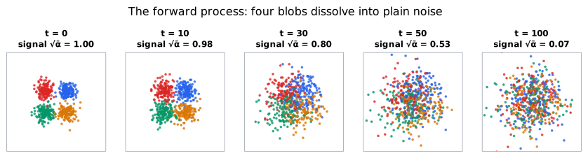
Reading it: each panel is the whole dataset, noised to the step in its title, with every dot keeping its blob's colour. Step 10 barely differs from the clean data (its signal share $\sqrt{\bar\alpha}$ is still 0.98). By step 30 the blobs have swollen into each other, though each colour still keeps to its own corner. By step 50 the colours overlap. At step 100 only 7% of the signal is left and the colours are thoroughly mixed: a round cloud of plain noise, the same cloud whatever data you started from. That last fact is what makes generation possible: we know how to draw from that cloud.
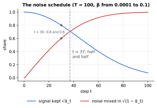
Reading it: the x-axis is the step. The blue curve is the signal share $\sqrt{\bar\alpha_t}$ and the red curve is the noise share $\sqrt{1 - \bar\alpha_t}$. The two dots at step 30 are the worked example's 0.8 and 0.6. The dashed line at step 37 is where signal and noise are equal. Early steps change little (the curves are flat at the left), so the network gets plenty of practice on nearly clean data, where the fine detail lives.
In code: linear_schedule builds the list of $\beta_t$ as a NoiseSchedule, whose NoiseSchedule.alpha_bars is the running product; noise_step is one step and add_noise is the shortcut.
Why it matters in practice. The forward process has no parameters and needs no training. Its only job is to manufacture unlimited practice material, and thanks to the shortcut, any clean example can be turned into a practice question at any noise level in one line.
Step 2: learning to denoise
Everyday picture. A photo restorer wants to practise removing specks of dust. They take clean photos and sprinkle dust on them themselves, keeping a note of exactly where every speck went. Now they can practise all day: guess where the dust is, then check against the note. The homework is unlimited and every answer is known.
Tiny worked example. Take the pixel from before: $x_0 = 2.0$, noise $\varepsilon = 0.5$, step 30, so $x_{30} = 1.9$. The network is shown only $x_{30} = 1.9$ and the step number 30, and asked: "what noise was added?" The right answer is 0.5. If it guesses 0.4, it is off by 0.1 and scores $(0.5 - 0.4)^2 = 0.01$. Lower is better.
Why guess the noise rather than the clean value? The two are equivalent: given $x_t$, $t$ and the noise, the clean value follows by undoing the shortcut, $x_0 = (1.9 - 0.6 \cdot 0.5) / 0.8 = 2.0$. Guessing the noise simply works better in practice, because the target always has the same size (a standard-normal draw), whatever the step.
flowchart LR
  D["pick a real point x₀"] --> MIX
  T["pick a random step t"] --> MIX
  E["draw noise ε"] --> MIX["mix with the shortcut<br/>x_t = √ᾱ_t x₀ + √(1 − ᾱ_t) ε"]
  MIX --> NET["network ε_θ<br/>sees x_t and t"]
  NET --> G["guess ε̂"]
  G --> L["loss ‖ε − ε̂‖²"]
  E --> L
  L --> U["nudge the weights<br/>(backprop + Adam)"]
Reading it: three random choices feed in from the left: which example,
which step, which noise. The shortcut mixes them into a noisy point. The
network sees only the noisy point and the step (not the noise, and not the
clean point). The noise takes the lower path straight to the loss, where the
guess is graded against it. Everything after the loss is ordinary training,
exactly as in primer.ml.neural_net.
Level 3: the formula and its symbols
$$ L(\theta) = \mathbb{E}_{x_0,\, t,\, \varepsilon}\Big[\, \big\| \varepsilon - \varepsilon_\theta(x_t, t) \big\|^2 \,\Big] $$
Symbols
| Symbol | Meaning here | In the example |
|---|---|---|
| $\theta$ | "theta": all of the network's weights, the knobs training turns | about 5,000 numbers here |
| $\varepsilon_\theta(x_t, t)$ | the network's guess of the noise, given the noisy point and the step; written $\hat\varepsilon$ ("epsilon hat") | (0.4, −0.8) |
| $\varepsilon$ | the noise that was really added (a 2-number vector in our world) | (0.5, −1.0) |
| $\varepsilon - \varepsilon_\theta$ | the error: how far off the guess is, per number | (0.1, −0.2) |
| $\lVert v \rVert^2$ | squared length: square every entry and add them up | $0.1^2 + 0.2^2 = 0.05$ |
| $\mathbb{E}_{x_0, t, \varepsilon}[\ldots]$ | expectation: the average over many random choices of example, step and noise; in code, the average over a batch | the batch average |
| $L(\theta)$ | the loss: one number saying how bad the guesses are with these weights | about 0.6 after training |
In words: "over many random examples, steps and noises, average how far the network's noise guess is from the real noise, measured as squared distance."
With the numbers: true noise (0.5, −1.0), guess (0.4, −0.8): error (0.1, −0.2), squared length $0.01 + 0.04 = 0.05$. A network that always guesses zero scores the average of $\varepsilon_1^2 + \varepsilon_2^2$, which is 1 + 1 = 2 (each standard-normal number has variance 1). That is the score to beat.
Level 3: in Python
In Python:
import random
eps = [0.5, -1.0]
guess = [0.4, -0.8]
# ‖ε − ε̂‖²: square each error and add
round(sum((e - g) ** 2 for e, g in zip(eps, guess)), 2)  # → 0.05
# the baseline: always guessing 0, averaged over many draws of 2-D noise
random.seed(0)
draws = [random.gauss(0, 1) ** 2 + random.gauss(0, 1) ** 2 for _ in range(100_000)]
round(sum(draws) / len(draws), 1)  # → 2.0
This is plain regression (predicting numbers, graded by squared error), the most stable kind of training there is. There is no opponent to balance and no trick: that is a big part of why diffusion displaced GANs.
The network. Our denoiser is a small multi-layer network: the noisy
point (2 numbers), plus the step turned into 8 numbers of sines and cosines
(a single number "30" is hard for a small network to use; a spread of waves
at different speeds is easy, the same trick as the sinusoidal positions in
primer.ml.positional), go through two hidden layers of 64 ReLU units
and come out as 2 numbers, the noise guess. It trains for 1,500 steps of
Adam (primer.ml.optimizers) on batches of 256, in about half a second.
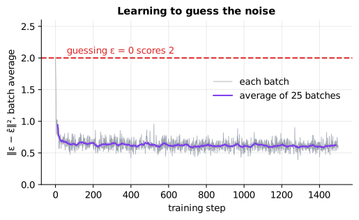
Reading it: the x-axis is training steps and the y-axis is the batch's average squared error. The dashed red line at 2 is the "always guess zero" baseline, and the untrained network starts right on it (its last layer starts near zero). The loss plunges within a hundred steps, then creeps down. It never reaches 0, and cannot: at low noise levels the noise is hidden inside the blob's own natural spread, so even a perfect network can only guess its average. The floor near 0.6 is that honest uncertainty, not a failure.
What the noise guess really is: the score
Flip the noise guess around and it becomes an arrow pointing toward the data. If the noise pushed the point up and to the right, the way back is down and to the left. That arrow has a name, the score: at any point, the direction in which the data gets more crowded, fastest. Learning to guess noise is secretly learning the score at every noise level, which is why diffusion models are also called score-based models, and why the training trick is called denoising score matching.
Level 3: the formula and its symbols
$$ \nabla_{x} \log p_t(x_t) \;\approx\; -\,\frac{\varepsilon_\theta(x_t, t)}{\sqrt{1 - \bar\alpha_t}} $$
Symbols
| Symbol | Meaning here | In the example |
|---|---|---|
| $p_t(x)$ | how crowded the noisy data is at point $x$ at step $t$ (its probability density) | the standard bell curve |
| $\log p_t$ | the logarithm of that density; crowdedness on a scale where multiplying becomes adding | $-x^2/2$ + a constant |
| $\nabla_x$ | "grad": the slope, in every direction, as $x$ moves; for one number, just the slope | slope of $-x^2/2$ is $-x$ |
| $\nabla_x \log p_t$ | the score: which way is uphill in crowdedness | $-1.5$ at $x = 1.5$ |
| $\varepsilon_\theta$ | the network's noise guess | 0.9 |
| $\sqrt{1-\bar\alpha_t}$ | the noise share, which converts "noise" units into "distance" units | 0.6 |
| $\approx$ | "approximately equal": exact for a perfect guesser |
In words: "the direction toward the data is the noise guess, flipped and divided by the noise share."
With the numbers: take data that is already standard-normal, so every noisy version is the plain bell curve, whose score at $x$ is $-x$ (the slope of $-x^2/2$). At $x_t = 1.5$ with $\bar\alpha_t = 0.64$, the best possible noise guess is $0.6 \times 1.5 = 0.9$, and the formula gives $-0.9 / 0.6 = -1.5$: exactly the score, pointing back toward the crowd at 0.
Level 3: in Python
In Python:
import math
x_t, alpha_bar = 1.5, 0.64
# the best noise guess for standard-normal data: √(1 − ᾱ) · x_t
eps_hat = math.sqrt(1 - alpha_bar) * x_t
round(eps_hat, 2)  # → 0.9
# −ε̂ / √(1 − ᾱ): the score, which for the bell curve is −x
round(-eps_hat / math.sqrt(1 - alpha_bar), 2)  # → -1.5
In code: DenoiserMLP is the network with its hand-written backward pass (denoiser_gradient_check compares it with finite differences), time_features turns the step into waves, train_noise_predictor is the training loop in the diagram and returns a NoisePredictor, and noise_to_score is the score formula.
Why it matters in practice. This loss, a squared error on guessed noise, is the training loss of the original DDPM paper and of the first Stable Diffusion models. The network is far bigger and the data is images, but the training loop is the boxes above.
Step 3: sampling, running the process backwards
Everyday picture. Back to the sculptor. Look at the block, guess which bits are "not horse", chip away a small part of them, look again. Never chip away everything you think is wrong at once: the guess is rough when the block is rough, and it gets better as the shape emerges.
Tiny worked example. A point sits at $x_t = 1.0$ at a step with $\beta_t = 0.19$ and $\bar\alpha_t = 0.75$. The network guesses the noise in it is $\hat\varepsilon = 0.5$. One step back removes a scaled share of that guess, undoes the shrinking, and (except on the very last step) adds a little fresh noise.
Level 3: the formula and its symbols
$$ x_{t-1} = \frac{1}{\sqrt{1-\beta_t}} \left( x_t - \frac{\beta_t}{\sqrt{1 - \bar\alpha_t}}\, \hat\varepsilon \right) + \sqrt{\beta_t}\; z $$
Symbols
| Symbol | Meaning here | In the example |
|---|---|---|
| $x_t$ | the current, noisier point | 1.0 |
| $\hat\varepsilon$ | the network's noise guess, $\varepsilon_\theta(x_t, t)$ | 0.5 |
| $\beta_t$ | this step's noise dose, from the schedule | 0.19 |
| $\frac{\beta_t}{\sqrt{1-\bar\alpha_t}}$ | how much of the guess belongs to this one step: only a sliver of all the noise was added here | $0.19 / 0.5 = 0.38$ |
| $\frac{1}{\sqrt{1-\beta_t}}$ | undo this step's shrink | $1/0.9$ |
| $z$ | fresh standard-normal noise; 0 on the final step | 0 or 0.5 |
| $\sqrt{\beta_t}\, z$ | a small random wobble | $0.436 \cdot 0.5 = 0.218$ |
| $x_{t-1}$ | the slightly cleaner point | 0.9, or 1.118 with the wobble |
In words: "subtract this step's share of the guessed noise, scale back up, and add a small fresh wobble."
With the numbers: $(1.0 - 0.38 \times 0.5) / 0.9 = 0.81 / 0.9 = 0.9$; with the wobble $z = 0.5$: $0.9 + 0.218 = 1.118$.
Level 3: in Python
In Python:
import math
x_t, eps_hat = 1.0, 0.5
beta, alpha_bar = 0.19, 0.75
# remove this step's share of the guessed noise, then undo the shrink
mean = (x_t - beta / math.sqrt(1 - alpha_bar) * eps_hat) / math.sqrt(1 - beta)
round(mean, 4)  # → 0.9
# add a small fresh wobble z
z = 0.5
round(mean + math.sqrt(beta) * z, 4)  # → 1.1179
Why add noise while trying to remove it? The network's guess is an average over every clean point that could have produced $x_t$. Stepping to that average would drift every sample toward the safe, blurry middle. The fresh wobble keeps each sample committed to one specific possibility, so the samples spread out over the whole data, as the real data does. This recipe is DDPM (denoising diffusion probabilistic models).
flowchart LR
  N["x_T: draw pure noise"] --> G["network guesses<br/>the noise ε̂ at step t"]
  G --> R["remove this step's share,<br/>undo the shrink"]
  R --> W["add a small fresh wobble<br/>(not on the last step)"]
  W --> Q{"t = 0?"}
  Q -- "no: t ← t − 1" --> G
  Q -- "yes" --> OUT["x₀: a new sample"]
Reading it: the loop runs once per step, $T = 100$ times here and 1,000 in the original paper. Each lap costs one full run of the network, so the number of laps is the price of a sample. Keep that in mind: the rest of the lesson is largely about making that loop shorter.
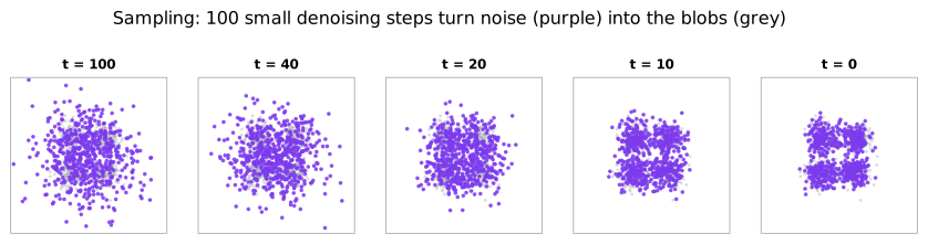
Reading it: grey dots are the real data, purple dots are 600 samples being generated, shown at five moments of the backwards run. For the first half almost nothing seems to happen: the network makes coarse, whole-cloud decisions while the noise is still loud. Between steps 20 and 10 the cloud splits toward the four corners, and the last few steps tighten each group onto its blob. Nobody told the network there were four blobs; it learned that from guessing noise.
Fewer steps: jump, don't crawl (DDIM)
Everyday picture. A sculptor in a hurry doesn't chip a sliver per look. They glance at the block, picture the finished horse, then rough the block out to a state only slightly less finished than that, and look again. Big confident moves, a handful of looks.
Tiny worked example. From the Step 1 pixel: $x_t = 1.9$ at $\bar\alpha_t = 0.64$, and suppose the network guesses the noise perfectly, $\hat\varepsilon = 0.5$. First predict the finished value, then re-noise it to a much quieter level, $\bar\alpha_s = 0.96$, reusing the same noise guess instead of drawing new noise.
Level 3: the formula and its symbols
$$ \hat x_0 = \frac{x_t - \sqrt{1-\bar\alpha_t}\;\hat\varepsilon}{\sqrt{\bar\alpha_t}} \qquad\qquad x_s = \sqrt{\bar\alpha_s}\;\hat x_0 + \sqrt{1-\bar\alpha_s}\;\hat\varepsilon $$
Symbols
| Symbol | Meaning here | In the example |
|---|---|---|
| $x_t$ | the current point, at step $t$ | 1.9 |
| $\hat\varepsilon$ | the network's noise guess | 0.5 |
| $\hat x_0$ | "x-zero hat": the predicted clean point, from undoing the shortcut | 2.0 |
| $s$ | the earlier step to jump to; any step before $t$, not just $t - 1$ | 96% signal |
| $\bar\alpha_t, \bar\alpha_s$ | the signal left at steps $t$ and $s$ | 0.64 and 0.96 |
| $x_s$ | the point after the jump: the predicted clean point, re-noised lightly | 2.06 |
In words: "guess the finished point by undoing the shortcut, then walk back to a quieter noise level along the same noise direction, with no fresh randomness."
With the numbers: $\hat x_0 = (1.9 - 0.6 \cdot 0.5) / 0.8 = 1.6 / 0.8 = 2.0$, then $x_s = \sqrt{0.96} \cdot 2.0 + \sqrt{0.04} \cdot 0.5 = 1.960 + 0.1 = 2.06$. Jump to $\bar\alpha_s = 1$ and you land on $\hat x_0$ itself.
Level 3: in Python
In Python:
import math
x_t, eps_hat = 1.9, 0.5
alpha_bar_t, alpha_bar_s = 0.64, 0.96
# x̂₀: undo the shortcut to predict the clean point
x0_hat = (x_t - math.sqrt(1 - alpha_bar_t) * eps_hat) / math.sqrt(alpha_bar_t)
round(x0_hat, 4)  # → 2.0
# x_s: re-noise it lightly, along the same noise direction
round(math.sqrt(alpha_bar_s) * x0_hat + math.sqrt(1 - alpha_bar_s) * eps_hat, 4)  # → 2.0596
This is DDIM (denoising diffusion implicit models). It uses the very same trained network; only the sampling loop changes. Because it adds no fresh noise, the same starting noise always gives the same sample, and it can take 20 jumps instead of 100 small steps. On the blobs, 20 DDIM jumps land as close to the data as 100 DDPM steps (the spec checks both).
In code: ddpm_step and ddpm_sample are the small-step sampler (ddpm_trajectory keeps snapshots for the figure); ddim_step and ddim_sample are the jumping one; two_way_distance measures how close samples land to the data, in both directions, so piling every sample onto one blob can't score well.
Why it matters in practice. Sampling cost is the number of network calls. The original DDPM used 1,000; samplers like DDIM brought that to about 20 to 50, which is what made diffusion usable in products. Pushing toward a handful of steps is the next idea.
Step 4: flow matching, the straight road
Everyday picture. Diffusion's road from noise to data is a winding mountain path set by the schedule. Flow matching asks: why not draw a straight line from each noise point to a data point, and learn the current that carries you along it? The network becomes a map of arrows, like a weather map of wind: at every place and time, it says which way to drift, and how fast. To generate, drop a leaf (a noise point) on the map and let it drift.
One warning about labels. In flow-matching papers, and in this section, $x_0$ is the noise and $x_1$ is the data, and time runs from 0 (noise) to 1 (data). That is the opposite of the diffusion sections above, where $x_0$ was the clean data.
Tiny worked example. Noise point $x_0 = -1$, data point $x_1 = 2$. The straight line between them passes, a quarter of the way along, through $0.75 \cdot (-1) + 0.25 \cdot 2 = -0.25$. The speed along the line is constant: it covers the distance $2 - (-1) = 3$ in one unit of time, so the velocity is 3 everywhere on it. The network is trained to output 3 when shown the point $-0.25$ at time 0.25.
Level 3: the formula and its symbols
$$ x_t = (1 - t)\, x_0 + t\, x_1 \qquad\qquad L(\theta) = \mathbb{E}_{x_0,\, x_1,\, t}\Big[\, \big\| v_\theta(x_t, t) - (x_1 - x_0) \big\|^2 \,\Big] $$
Symbols
| Symbol | Meaning here | In the example |
|---|---|---|
| $x_0$ | a noise point (standard normal) | −1 |
| $x_1$ | a real data point, paired with the noise at random | 2 |
| $t$ | time along the line, from 0 (noise) to 1 (data), drawn at random in training | 0.25 |
| $x_t$ | the point on the straight line at time $t$ | −0.25 |
| $x_1 - x_0$ | the velocity of that line: where to go, and how fast; the same at every $t$ | 3 |
| $v_\theta(x_t, t)$ | the network's guessed velocity at that place and time | say 2.5 |
| $\lVert \ldots \rVert^2$, $\mathbb{E}$ | squared length and average over many random draws, as in Step 2 | $(2.5 - 3)^2 = 0.25$ |
In words: "pick a noise point, a data point and a time; find the point that far along the straight line between them; train the network to output the line's direction and speed there."
With the numbers: $x_{0.25} = 0.75 \cdot (-1) + 0.25 \cdot 2 = -0.25$; target velocity $2 - (-1) = 3$; a guess of 2.5 scores $(2.5 - 3)^2 = 0.25$.
Level 3: in Python
In Python:
x0, x1, t = -1.0, 2.0, 0.25
# (1 − t) x₀ + t x₁: the point on the straight line
x_t = (1 - t) * x0 + t * x1
x_t  # → -0.25
# x₁ − x₀: the velocity to learn
x1 - x0  # → 3.0
# a guess of 2.5 is graded by squared error
(2.5 - (x1 - x0)) ** 2  # → 0.25
To generate, start from noise at $t = 0$ and follow the arrows in a few Euler steps (the simplest way to follow a velocity: move in a straight line for a short time, then look again):
Level 3: the formula and its symbols
$$ x_{t+h} = x_t + h\; v_\theta(x_t, t) $$
Symbols
| Symbol | Meaning here | In the example |
|---|---|---|
| $h$ | the step size in time; $N$ equal steps means $h = 1/N$ | 0.75 |
| $v_\theta(x_t, t)$ | the velocity the network reports here and now | 3 |
| $x_{t+h}$ | where you are after moving for time $h$ | 2.0 |
In words: "move for a short time in the direction, and at the speed, the network says."
With the numbers: from $x_{0.25} = -0.25$, one step of $h = 0.75$ at velocity 3 gives $-0.25 + 0.75 \times 3 = 2.0$: exactly the data point. On a straight line, one step of any size is exact, because there is no bend to cut.
Level 3: in Python
In Python:
x_t, v, h = -0.25, 3.0, 0.75
# x + h v: one Euler step
x_t + h * v  # → 2.0
flowchart LR
  subgraph TRAIN["Training"]
    direction LR
    P["pair noise x₀<br/>with data x₁"] --> L1["point on the line<br/>(1 − t) x₀ + t x₁"]
    L1 --> V["network guesses v"]
    V --> LOSS["loss ‖v − (x₁ − x₀)‖²"]
  end
  subgraph SAMPLE["Sampling"]
    direction LR
    Z["draw noise, t = 0"] --> STEP["x ← x + h · v(x, t)"]
    STEP --> C{"t = 1?"}
    C -- no --> STEP
    C -- yes --> S["a new sample"]
  end
Reading it: training (top) is the same shape as diffusion's: random choices in, a point in between, a squared-error guess. The difference is the target: a velocity along a straight line rather than hidden noise. Sampling (bottom) is a plain loop of Euler steps from $t = 0$ to $t = 1$, with no schedule, no shrink factors and no fresh noise.
There is a catch, and it is instructive. Many different straight lines pass through the same point (from different noise to different data), so the network cannot know which one it is on. It learns the average of their velocities. The learned paths are therefore only roughly straight: they bend, because two paths can never cross (at any point the network gives one velocity, so two paths that met would continue together).
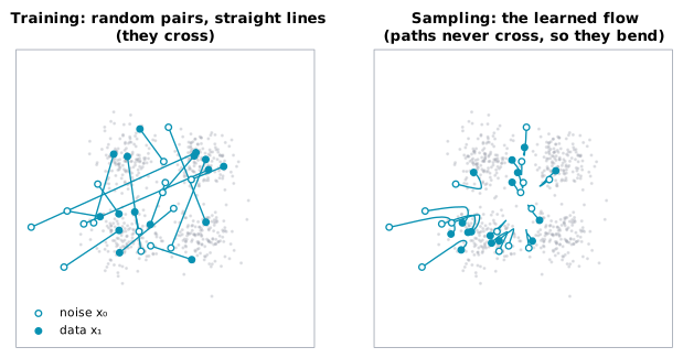
Reading it: hollow circles are noise, filled circles are where each path ends. On the left are training pairs: every line is straight, but they criss-cross because noise and data were paired at random. On the right, the learned flow starts from the same noise. Its paths never cross, so they bend to share out the blobs, mostly near the end. The straighter the paths, the fewer Euler steps you need. That is why rectified flow retrains on the model's own (noise, sample) pairs, which no longer cross: each round makes the paths straighter, until one or two steps are enough.
The average also explains the extreme case. With a single Euler step from $t = 0$, every noise point moves by the average velocity toward "the data in general" and lands on the data's average: the empty middle of the four blobs (the spec checks it). Straight-line training does not make one step free; straight learned paths do.
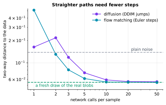
Reading it: the x-axis is network calls per sample and the y-axis is the two-way distance between samples and data (lower is better). The green floor is a fresh draw of the real blobs, as good as samples can get; the grey line is plain noise. At one or two calls neither method does much better than noise. Flow matching (teal) gets close to the floor within about 5 calls, while diffusion's DDIM jumps (purple) need about 10 to get as close. Same network size, same training time: the straighter paths need roughly half the steps.
In code: flow_point and flow_target build the training pairs, train_velocity_predictor trains a VelocityPredictor, euler_step and euler_sample follow it, and step_sweep measures both methods at each step count.
Why it matters in practice. Flow matching and rectified flow give a simpler recipe (no noise schedule to tune, just straight lines) and need fewer sampling steps. Stable Diffusion 3 is trained as a rectified flow, and many recent image and video generators follow. Under the hood it is the same family as diffusion: a network trained by squared error to point from noise toward data, followed step by step.
Step 5: conditioning and guidance, generating what you asked for
Everyday picture. A caricaturist draws a famous face by noticing what makes it different from an average face (the big chin, the eyebrows) and exaggerating exactly that difference. Guidance does the same: compare "what I'd draw if told what to draw" with "what I'd draw anyway", and push further in the direction of the difference.
Conditioning first: to ask for a specific corner, feed the label to the network as an extra input. Our labels are four corners, given as a one-hot vector (all zeros except a 1 in the chosen slot), plus a fifth slot that means "no label". A text-to-image model does the same with a sentence in place of a corner name.
Classifier-free guidance trains one network to answer both questions: in training, the label is hidden (replaced by "no label") on a random 20% of examples. At sampling time the network is asked twice per step, once with the label and once without, and the two guesses are mixed.
Tiny worked example. At some point during sampling, the guess without the label is $\hat\varepsilon_\varnothing = 0.2$ and the guess with the label "south-west" is $\hat\varepsilon_c = 0.5$. The label moves the guess by $0.5 - 0.2 = 0.3$. With guidance weight $w = 3$, move three times as far.
Level 3: the formula and its symbols
$$ \tilde\varepsilon = \hat\varepsilon_\varnothing + w \,\big(\hat\varepsilon_c - \hat\varepsilon_\varnothing\big) $$
Symbols
| Symbol | Meaning here | In the example |
|---|---|---|
| $\hat\varepsilon_\varnothing$ | the noise guess with the label hidden ($\varnothing$, "empty set", stands for "no label") | 0.2 |
| $\hat\varepsilon_c$ | the noise guess given the label $c$ | 0.5 |
| $\hat\varepsilon_c - \hat\varepsilon_\varnothing$ | what the label changes: the direction "more like $c$" | 0.3 |
| $w$ | the guidance weight (or guidance scale): 0 ignores the label, 1 is the plain labelled guess, above 1 exaggerates | 3 |
| $\tilde\varepsilon$ | "epsilon tilde": the guided guess, used in place of $\hat\varepsilon$ by the sampler | 1.1 |
In words: "start from the unlabelled guess and move $w$ times as far as the label would move it."
With the numbers: $0.2 + 3 \times (0.5 - 0.2) = 0.2 + 0.9 = 1.1$. With $w = 0$ it is 0.2 (the label is ignored); with $w = 1$ it is 0.5 (exactly the labelled guess).
Level 3: in Python
In Python:
eps_uncond, eps_cond = 0.2, 0.5
# ε̃ = ε̂_∅ + w (ε̂_c − ε̂_∅), for w = 0, 1 and 3
[round(eps_uncond + w * (eps_cond - eps_uncond), 2) for w in (0, 1, 3)]  # → [0.2, 0.5, 1.1]
flowchart LR
  X["noisy point x_t, step t"] --> A["network, label hidden"]
  X --> B["network, label = south-west"]
  A --> U["ε̂_∅"]
  B --> C["ε̂_c"]
  U --> MIX["ε̃ = ε̂_∅ + w (ε̂_c − ε̂_∅)"]
  C --> MIX
  MIX --> STEP["one sampler step<br/>(DDIM or DDPM)"]
Reading it: each step runs the same network twice, once with the label hidden and once with it shown, which doubles the cost of a step. The two guesses meet in the mixing box, and only the mixed guess reaches the sampler, which is otherwise unchanged. Nothing new was trained for guidance: it is a choice made at sampling time.
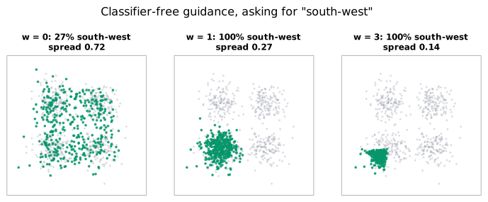
Reading it: grey dots are the data, green dots are samples asked for "south-west" at three guidance weights. At $w = 0$ the label is ignored, so samples land in all four corners, only about a quarter in the south-west. At $w = 1$ nearly all land in the right blob with roughly the real blob's spread. At $w = 3$ they are all on target but bunched into a tight knot, pushed to the side of the blob farthest from the other blobs: the most unmistakably south-west spot. That is guidance in one picture: more on-label, less varied, and exaggerated.
In code: network_inputs appends the one-hot label with its "no label" slot, train_noise_predictor hides labels at random when given them, guided_noise is the formula, ddim_sample applies it at every jump when given a label, and guidance_sweep measures the share on target and the spread at each weight.
Why it matters in practice. Text-to-image systems use guidance weights well above 1, because unguided samples follow the prompt only loosely. Turn it too high and images become oversaturated and samey, the image version of the tight knot above. The "guidance scale" slider in image tools is this $w$.
Step 6: scaling up to real images, video and audio
Everyday picture. An architect doesn't design a skyscraper by placing every brick. They draw a floor plan, small enough to think about, and a builder turns the plan into a building. Latent diffusion does the creative work on a small "plan" of the image, and a separate decoder builds the pixels.
Tiny worked example. A 512 × 512 colour image is $512 \times 512 \times 3
= 786{,}432$ numbers. An autoencoder (a network that squeezes an image
into a small code and rebuilds it; see primer.ml.generative.autoencoders)
shrinks each side by 8 and keeps 4 numbers per position: $64 \times 64 \times
4 = 16{,}384$ numbers. The denoiser now works on 48 times fewer numbers, and
every one of its many steps is that much cheaper.
Level 3: the formula and its symbols
$$ \text{shrink factor} = \frac{H \cdot W \cdot 3}{(H/f) \cdot (W/f) \cdot c} $$
Symbols
| Symbol | Meaning here | In the example |
|---|---|---|
| $H, W$ | image height and width in pixels | 512, 512 |
| 3 | colour channels: red, green, blue | 3 |
| $f$ | how much the autoencoder shrinks each side | 8 |
| $c$ | numbers kept per latent position (latent channels) | 4 |
| shrink factor | how many times fewer numbers the denoiser handles | 48 |
In words: "count the numbers in the image, count the numbers in its latent code, and divide."
With the numbers: $786{,}432 / 16{,}384 = 48$. The latent is then cut
into 2 × 2 patches, each patch becoming one token for a transformer:
$(64/2) \times (64/2) = 1{,}024$ tokens. A 16-frame video clip in the same
latent space is 16 times that, 16,384 tokens, and since attention compares
every token with every other (primer.ml.attention), it costs $16^2 = 256$
times as much.
Level 3: in Python
In Python:
H, W, f, c = 512, 512, 8, 4
pixels = H * W * 3
latents = (H // f) * (W // f) * c
pixels, latents  # → (786432, 16384)
# shrink factor
pixels / latents  # → 48.0
# 2 × 2 patches of the 64 × 64 latent: the transformer's tokens
tokens = (64 // 2) * (64 // 2)
tokens  # → 1024
# 16 video frames: 16× the tokens, 256× the attention pairs
(16 * tokens) ** 2 // tokens ** 2  # → 256
flowchart LR
  P["prompt: 'a red fox in snow'"] --> TE["text encoder<br/>(e.g. CLIP's text tower)"]
  TE --> TOK["text token vectors"]
  N["random latent noise<br/>64 × 64 × 4"] --> DEN
  TOK --> DEN["denoiser: a transformer<br/>over latent patches,<br/>attending to the text"]
  DEN -- "20 to 50 steps,<br/>with guidance" --> DEN
  DEN --> LAT["clean latent"]
  LAT --> DEC["autoencoder decoder"]
  DEC --> IMG["512 × 512 image"]
Reading it: follow the noise from the left. It is not an image but a
small latent, and all the sampling steps (the loop on the denoiser box)
happen in that cheap space. The prompt takes the upper path: a text
encoder, such as CLIP's text half (primer.ml.embeddings.contrastive),
turns it into token vectors that the denoiser reads through
cross-attention (attention whose queries come from the image patches and
whose keys and values come from the text tokens). Guidance's "no label"
answer is simply an empty prompt. Only at the very end does the decoder
turn the latent into pixels, once.
Three more scale-ups follow the same pattern:
- The denoiser became a transformer. Early systems used a U-Net (a
convolutional network,
primer.ml.cnn_rnn); the diffusion transformer (DiT) cuts the latent into patches and treats them as tokens, so the scaling lessons of language models carry over. - Video adds a time axis: the latent is a stack of frames, and patches span space and time. It is the same denoising, with far more tokens.
- Audio is denoised as a spectrogram (a picture of sound: time across, pitch up, loudness as brightness) or as an audio autoencoder's latent.
Compared with the other generators in this part:
GAN (primer.ml.generative.gans) |
VAE (primer.ml.generative.autoencoders) |
Diffusion and flow matching | |
|---|---|---|---|
| Training | a generator against a critic: unstable | reconstruct plus stay near a simple code: stable | squared error on noise or velocity: stable |
| Samples | sharp | often blurry | sharp |
| Covers all of the data? | can mode collapse (ignore whole regions) | yes | yes |
| Cost of one sample | one network call | one network call | 5 to 50 network calls |
In code: latent_shrink counts pixels against latent numbers and patch_tokens counts a diffusion transformer's tokens, per frame.
Why it matters in practice. Latent space made high-resolution diffusion affordable on a single GPU, transformers made it scale, text encoders made it follow prompts, and guidance made it follow them closely. The price that remains is many network calls per sample, which is why step-reduction (DDIM, flow matching, distillation into few-step students) is where so much engineering effort goes.
In 20 seconds
- Forward process: mix data with a little Gaussian noise per step until only noise is left; the shortcut $x_t = \sqrt{\bar\alpha_t}\,x_0 + \sqrt{1-\bar\alpha_t}\,\varepsilon$ jumps to any step in one go.
- Training: show the network a noised example and the step; it guesses the noise; grade by squared error. Plain, stable regression, and secretly learning the score (the direction toward the data).
- Sampling: start from pure noise and repeatedly remove a little guessed noise (DDPM, with a fresh wobble each step), or take a few big deterministic jumps (DDIM).
- Flow matching: learn the velocity along straight lines from noise to data and follow it with Euler steps; straighter paths need fewer steps.
- Guidance: ask the same network with and without the label and push past the labelled guess; more on-prompt, less varied.
- At scale: denoise an autoencoder's small latent with a transformer that reads a text encoder's tokens; video and audio are the same idea with more tokens.
Self-test questions
Why does the network learn to guess the noise, rather than the clean picture? The two carry the same information: given the noisy point, the step and the noise, the clean point follows by undoing the shortcut. Guessing the noise works better in practice because the target is always the same size (a standard-normal draw) at every step, which makes one network easy to train across all noise levels. The noise guess, flipped and rescaled, is also the score: the direction toward the data.
Training only ever takes one jump from clean to noisy. Why does generation need many steps back? The noise guess is an average over every clean point that could have produced the noisy one. From heavy noise that average is vague, pointing at the middle of the data, so one big step lands on a blur (or, in our blobs, the empty middle). Small steps let the guess sharpen as the sample commits to one specific region, and the network is asked again at every stage.
Why does DDPM add fresh noise at each step, when the goal is to remove noise? Without it, every step moves toward the network's averaged guess and samples drift toward safe, typical, blurry results. The small fresh wobble keeps each sample exploring one specific possibility, so the samples cover all of the data. DDIM drops the wobble on purpose, trading that randomness for determinism and big jumps.
What does flow matching change, and why can it get away with fewer steps? It replaces the noise schedule with straight lines from noise to data and trains the network to output the velocity along them. Following a velocity with Euler steps is only exact on straight paths; the learned paths are straighter than diffusion's, so fewer steps cut fewer corners. They are not perfectly straight, because paths can't cross, which is what rectified flow's retraining fixes.
What does the guidance weight do, and what goes wrong if it is too large? It sets how far past the labelled guess to go, along the direction from the unlabelled guess to the labelled one. 0 ignores the prompt, 1 follows it plainly, above 1 exaggerates it, so samples match the prompt more reliably. Too large and samples become samey, over-saturated caricatures of the prompt, bunched into the most extreme examples.
Why do real image generators denoise in a latent space instead of on pixels? Most of an image's pixel values are fine texture that a decoder can fill in. An autoencoder shrinks a 512 × 512 image 48-fold into a latent that keeps the meaningful structure, and since sampling runs the denoiser dozens of times, every step becomes that much cheaper. The decoder runs just once, at the end.
When would you choose a GAN over a diffusion model? When one-shot speed matters most: a GAN makes a sample in a single network call, where diffusion needs several to dozens. Diffusion wins on training stability and on covering all of the data (GANs can mode-collapse), which is why it took over image generation; distillation is now closing its speed gap.
The papers behind this lesson
- Sohl-Dickstein et al., Deep Unsupervised Learning using Nonequilibrium Thermodynamics (2015): https://arxiv.org/abs/1503.03585. The original idea: destroy data slowly with noise, and learn to reverse the destruction.
- Song and Ermon, Generative Modeling by Estimating Gradients of the Data Distribution (2019): https://arxiv.org/abs/1907.05600. Generated samples by learning the score at many noise levels and following it.
- Ho, Jain and Abbeel, Denoising Diffusion Probabilistic Models (2020): https://arxiv.org/abs/2006.11239. The simple "guess the noise" loss and the sampler of Step 3, with the first high-quality image results. Annotated companion
- Song, Meng and Ermon, Denoising Diffusion Implicit Models (2020): https://arxiv.org/abs/2010.02502. Deterministic sampling with big jumps, using the same trained network. Annotated companion
- Song et al., Score-Based Generative Modeling through Stochastic Differential Equations (2020): https://arxiv.org/abs/2011.13456. Showed diffusion and score-based models are one family, described as continuous time processes. Annotated companion
- Ho and Salimans, Classifier-Free Diffusion Guidance (2022): https://arxiv.org/abs/2207.12598. Guidance from one network trained with and without the label, no separate classifier needed. Annotated companion
- Rombach et al., High-Resolution Image Synthesis with Latent Diffusion Models (2021): https://arxiv.org/abs/2112.10752. Denoising in an autoencoder's latent space, with text via cross-attention: the basis of Stable Diffusion. Annotated companion
- Peebles and Xie, Scalable Diffusion Models with Transformers (2022): https://arxiv.org/abs/2212.09748. Replaced the U-Net with a transformer over latent patches, and showed it improves with scale. Annotated companion
- Lipman et al., Flow Matching for Generative Modeling (2022): https://arxiv.org/abs/2210.02747. Trained continuous flows by regressing velocities along simple paths from noise to data. Annotated companion
- Liu, Gong and Liu, Flow Straight and Fast: Learning to Generate and Transfer Data with Rectified Flow (2022): https://arxiv.org/abs/2209.03003. Straight-line paths, and retraining on the model's own pairs to straighten the learned flow for few-step sampling. Annotated companion
- Esser et al., Scaling Rectified Flow Transformers for High-Resolution Image Synthesis (2024): https://arxiv.org/abs/2403.03206. Rectified flow with a transformer denoiser at scale: Stable Diffusion 3.
Further reading
- Ho, Jain and Abbeel, Denoising Diffusion Probabilistic Models (2020): https://arxiv.org/abs/2006.11239
- Song, Meng and Ermon, Denoising Diffusion Implicit Models (2020): https://arxiv.org/abs/2010.02502
- Ho and Salimans, Classifier-Free Diffusion Guidance (2022): https://arxiv.org/abs/2207.12598
- Lipman et al., Flow Matching for Generative Modeling (2022): https://arxiv.org/abs/2210.02747
- Liu, Gong and Liu, Rectified Flow (2022): https://arxiv.org/abs/2209.03003
- Rombach et al., Latent Diffusion Models (2021): https://arxiv.org/abs/2112.10752
- Peebles and Xie, Diffusion Transformers (2022): https://arxiv.org/abs/2212.09748
- Lilian Weng, What are Diffusion Models?: https://lilianweng.github.io/posts/2021-07-11-diffusion-models/
- Hugging Face, The Annotated Diffusion Model (DDPM, line by line in code): https://huggingface.co/blog/annotated-diffusion
- Hugging Face Diffusers documentation: https://huggingface.co/docs/diffusers/index
1r""" 2# Diffusion and flow matching: turning noise into data one small step at a time 3 4Run: `python -m primer.ml.generative.diffusion` 5 6New to the notation (vectors, sums, square roots, averages)? Every symbol is 7decoded where it appears, and `primer.notation` teaches them all from zero. 8This lesson trains small networks, so `primer.ml.neural_net` (how a network 9learns) is the one to read first. 10 11## Level 1: The practitioner's guide 12 13**In one sentence.** A diffusion model generates by learning one modest 14skill, "remove a little noise from this noisy example", and running it many 15times starting from pure noise; flow matching is the same idea along 16straight paths with fewer steps; together they are the engine inside 17today's image, video and audio generators, and the settings you meet 18(steps, guidance scale, resolution, seed) are the dials of that engine. 19 20**When you need it.** You need this lesson the moment you generate or edit 21images, video or audio: whether you call a hosted model or run an open one, 22the choices you make (which model family, how many steps, what guidance 23scale, what size, which sampler) are the ones below, and the bill and the 24artefacts follow from them. You don't need diffusion for text (language 25models generate one token at a time), for a one-pass generator in a 26real-time loop (a GAN or a distilled few-step model, see 27`primer.ml.generative.gans`), or for a tiny domain with a handful of 28factors (a VAE will do, see `primer.ml.generative.autoencoders`). The number 29that shows the naive approach failing: ask this lesson's trained model for 30a sample in a single step and every sample lands on the data's average, the 31empty middle between the four blobs (mean distance from the centre 0.08); 32give it 20 well-placed jumps and its samples sit as close to the data as a 33fresh draw of the data itself (0.056 against 0.055). 34 35**Your options.** From the least commitment to the most: 36 37| Option | What it does | What it guarantees | What it costs | Where it lives | 38|---|---|---|---|---| 39| A hosted image, video or audio model | Prompt in, sample out; you set steps, guidance, size and seed | No infrastructure; the vendor's sampler and safety checks | A price per sample, and only the dials the API exposes | The vendor's API | 40| An open latent-diffusion model in a pipeline | A pretrained denoiser, text encoder and autoencoder you run | Full control of sampler, steps, guidance, seed and adapters | A GPU with enough memory; defaults of 50 steps and guidance 7.5 in diffusers | Your server | 41| A faster sampler on the same model | DDIM or a higher-order solver takes big deterministic jumps | The same trained weights, 10 to 50 times faster than the original 1,000 steps | Quality falls off below about 10 calls | A setting in the pipeline | 42| A flow-matching or rectified-flow model | Trained to follow straight paths from noise to data | Fewer steps for the same quality (near the floor by 5 calls here, against 10 for diffusion) | A model trained that way, such as Stable Diffusion 3 | The model family you download | 43| A distilled few-step model | A student trained to match the full model in 1 to 4 steps, often with an adversarial loss | Real-time sampling | Some variety and detail; a teacher and a distillation run | The fast path beside the full model | 44| Your own diffusion model | This lesson's training loop on your own data | A generator for a narrow domain nobody has published | Data, a training run (half a second for the lesson's toy; hundreds of GPU-days for pixel-space image models), an autoencoder if the data is large | Your training loop | 45 46**How to choose.** Start from the latency you can afford, then set the 47dials in this order. 48 49- Steps first. The number of network calls is the price of a sample. Start 50 at the pipeline default (50 in diffusers), halve it while the output 51 holds, and reach for a flow model or a distilled one when you need fewer 52 than about 10. 53- Guidance scale next. 0 ignores the prompt (27% of samples on the asked-for 54 blob here), 1 follows it plainly (100% on target, with the data's own 55 spread), and above 1 exaggerates it: at 3 every sample is on target but 56 bunched into a knot at the far edge of the blob, spread 0.14 against the 57 real 0.27. Text-to-image models default to well above 1 (7.5 in 58 diffusers), because unguided samples follow prompts loosely; raise it for 59 obedience, lower it for variety. 60- Resolution: generate at the size the model was trained on (Stable 61 Diffusion 1.x was trained on 512 × 512 images), and upscale afterwards. 62 Every doubling of side length quadruples the latent and the attention 63 cost more than that. 64- Determinism: DDIM and flow samplers add no fresh noise, so one seed gives 65 one image, which is what makes a seed reproducible and an image editable 66 by re-running with a changed prompt. 67- Whatever you pick, judge the output on variety as well as quality. Every 68 dial that makes samples match the prompt better makes them more alike. 69 70**What it costs.** Latency is steps times the cost of one denoiser call, 71and guidance doubles the calls per step (the network runs once with the 72prompt and once without). Working in an autoencoder's latent cuts each call 7348-fold for a 512 × 512 image (786,432 numbers down to 16,384), which is 74what made high-resolution diffusion affordable on one GPU. Video multiplies 75it back: 16 frames of the same latent are 16 times the tokens and, because 76attention compares every token with every other, 256 times the attention 77work. The denoiser itself is now usually a transformer over latent patches, 78and the DiT paper found that more compute per sample (a deeper or wider 79model, or more tokens) gives lower FID, down to 2.27 on 256 × 256 80ImageNet. Training a real model is the expensive part: pixel-space diffusion 81"often consumes hundreds of GPU days" in the latent-diffusion paper's own 82words, which is why the pretrained autoencoder and the latent exist. The 83training loss itself is plain squared-error regression with no adversary, 84which is why the runs are stable and why diffusion displaced GANs. 85 86**What breaks.** 87 88- **Too few steps.** Below roughly 10 calls a diffusion sampler's output 89 drifts toward the average (the empty middle here; blur or mush in images). 90 Use a flow or distilled model instead of starving a diffusion one. 91- **Guidance too high.** Oversaturated, samey, exaggerated images, the 92 image version of the tight knot at weight 3; the diffusers documentation 93 puts it as prompt adherence "at the expense of lower image quality". Pull 94 it back toward the default. 95- **Guidance too low.** The prompt is followed loosely or not at all, as at 96 weight 0. A guidance scale of 1 or below switches guidance off. 97- **The wrong size.** A model asked for a resolution or aspect ratio far 98 from its training size composes badly (repeated subjects, stretched 99 scenes). Generate at the native size and upscale. 100- **A mismatched autoencoder or scale.** The latent must be decoded by the 101 autoencoder the denoiser was trained with, with the library's scaling 102 factor applied both ways, or the output is junk; see 103 `primer.ml.generative.autoencoders`. 104- **Averaging without the wobble.** DDPM adds a small fresh noise each step 105 so samples commit to one possibility; a sampler that only ever steps to 106 the network's average drifts to the safe, blurry middle. Deterministic 107 samplers avoid this by jumping along the predicted noise direction, not 108 to the mean. 109- **Cost that scales with frames.** A video request costs attention 110 quadratically in its token count; a short clip at a modest size is many 111 images' worth of compute, and the bill follows. 112 113**In the wild.** Stable Diffusion is the open reference: an 860-million 114parameter U-Net denoising a 64 × 64 × 4 latent, conditioned through 115cross-attention on a frozen CLIP ViT-L/14 text encoder, trained on 116512 × 512 images, and run through Hugging Face diffusers with 50 steps and 117guidance 7.5 by default. DDIM (Song, Meng and Ermon) gave the 10 to 50 118times faster deterministic sampler every pipeline offers; classifier-free 119guidance (Ho and Salimans) is the guidance-scale slider, trading variety 120for fidelity with no separate classifier; DiT (Peebles and Xie) replaced 121the U-Net with a transformer over latent patches and showed it scales; 122Stable Diffusion 3 (Esser et al.) trains a transformer as a rectified flow 123with 16-channel latents; Adversarial Diffusion Distillation turns a 124foundation model into a one-to-four-step sampler. Video generators run the 125same denoiser over patches that span space and time, and audio generators 126denoise a spectrogram or an audio autoencoder's latent. Every paper is 127linked at the end of the lesson. 128 129**Go deeper.** Level 2 builds the whole engine on four blobs of dots: the 130forward process and its one-jump shortcut, the noise-guessing loss and why 131it is secretly learning the direction toward the data, DDPM and DDIM 132sampling step by step, flow matching along straight lines, guidance with 133its knot, and the latent-and-patches arithmetic behind real systems. If 134you only needed to set the dials, you are done. 135 136## Level 2: How it works, from scratch 137 138Imagine a sculptor who cannot carve a statue in one go. Hand them a shapeless 139block and ask for a horse, and they freeze. But hand them a *slightly rough* 140horse, and they can always make it a little less rough: smooth this bump, 141deepen that line. Now chain that one modest skill. Start from a shapeless 142block, make it a bit more horse-like, then a bit more, a hundred times over, 143and a horse comes out. 144 145A diffusion model is that sculptor. It never learns "draw a picture from 146nothing", which is very hard. It learns "here is a picture with a little too 147much noise in it: take some of the noise away", which is much easier. And 148the practice material is free: take any real picture, add noise yourself, 149and you know exactly what the answer should be. 150 151```mermaid 152flowchart LR 153 D["Real data<br/>(a photo)"] -- "add a little noise,<br/>T times (fixed, no learning)" --> N["Pure noise<br/>(TV static)"] 154 N -- "remove a little noise,<br/>T times (learned)" --> S["A new sample<br/>(a photo no one took)"] 155``` 156 157**Reading it:** the top arrow is the *forward process*: it destroys data by 158adding noise a little at a time, and it involves no learning at all. The 159bottom arrow runs the same road backwards, and that direction is what the 160network learns. At generation time only the bottom arrow runs, starting 161from fresh noise, so every run ends at a different, new sample. 162 163**The tiny world this lesson works in.** A real image is a long list of 164numbers, one per pixel colour. To keep everything small enough to see, our 165"images" have just two numbers, so each one is a dot on a flat plane. The 166real data is four round blobs of dots, one in each corner (north-east, 167north-west, south-west, south-east), 600 dots in all. The job: learn to make 168*new* dots that land in the blobs, starting from random noise. Every idea 169below works unchanged on a 512 × 512 colour image; it just has 786,432 170numbers per "dot" instead of 2. 171 172Notice one thing about the blobs now, because it matters later: their 173average is the empty middle. A model that plays safe and outputs "the 174average answer" puts its dots where no real data lives. The same failure 175makes blurry images: the average of many sharp faces is a blur. 176 177## Step 1: the forward process, adding noise a little at a time 178 179**Everyday picture.** Think of an old television slowly losing its signal. 180Turn the static dial up one notch: the picture fades a little and a little 181snow creeps in. Turn it a hundred notches and you see only snow, and nothing 182in it tells you what the programme was. 183 184**Tiny worked example.** Follow one pixel whose clean value is $x_0 = 2.0$. 185Each step keeps most of the signal and mixes in a little fresh random noise. 186The **noise** is a random number drawn from a **standard normal 187distribution**: the bell curve centred on 0 whose typical size is 1 (values 188like 0.5, −1.2 and 0.1 are common, 3 is rare). Say step 1 mixes in a share 189$\beta = 0.1$ of noise, and the random draw is $\varepsilon = 0.5$. 190 191$$ 192x_t = \sqrt{1 - \beta_t}\; x_{t-1} + \sqrt{\beta_t}\; \varepsilon 193$$ 194 195**Symbols** 196 197| Symbol | Meaning here | In the example | 198|---|---|---| 199| $t$ | the step number, from 1 to $T$ (the last step) | 1 | 200| $x_{t-1}$ | the value before this step ($x_0$ is the clean data) | 2.0 | 201| $x_t$ | the value after this step | 2.06 | 202| $\beta_t$ | "beta": how much noise this step mixes in, a number between 0 and 1 | 0.1 | 203| $\sqrt{1-\beta_t}$ | how much of the old value survives: it shrinks a little | $\sqrt{0.9} = 0.949$ | 204| $\varepsilon$ | "epsilon": fresh noise drawn from the standard normal bell curve | 0.5 | 205| $\sqrt{\beta_t}$ | how much noise is mixed in | $\sqrt{0.1} = 0.316$ | 206 207**In words:** "shrink the old value a little, then add a little random noise." 208 209**With the numbers:** $x_1 = \sqrt{0.9} \cdot 2.0 + \sqrt{0.1} \cdot 0.5 = 2101.897 + 0.158 = 2.06$. 211 212**In Python:** 213 214```python 215import math 216x_prev, beta, eps = 2.0, 0.1, 0.5 217# √(1 − β) x_{t−1}: shrink the old value 218round(math.sqrt(1 - beta) * x_prev, 3) # → 1.897 219# √β ε: the noise mixed in 220round(math.sqrt(beta) * eps, 3) # → 0.158 221round(math.sqrt(1 - beta) * x_prev + math.sqrt(beta) * eps, 2) # → 2.06 222``` 223 224Why the square roots? A value's **variance** (its typical squared size) is 225what matters, and variances of independent things add. If the old value has 226variance 1, the new one has variance $(1 - \beta) \cdot 1 + \beta \cdot 1 = 1$: 227exactly 1 again. The square roots keep every step at the same overall size, 228so after many steps the value is noise of size 1, not a number that has 229blown up or faded to zero. 230 231### The shortcut: jump straight to any step 232 233Running $t$ steps one by one is slow, and training needs noisy examples at 234every step. Luckily, adding noise twice is the same as adding it once in a 235bigger dose, so there is a formula that jumps straight to step $t$. First, 236multiply up how much signal survives every step so far: 237 238$$ 239\bar\alpha_t = \prod_{s=1}^{t} (1 - \beta_s) 240\qquad\qquad 241x_t = \sqrt{\bar\alpha_t}\; x_0 + \sqrt{1 - \bar\alpha_t}\; \varepsilon 242$$ 243 244**Symbols** 245 246| Symbol | Meaning here | In the example | 247|---|---|---| 248| $1 - \beta_s$ | the share of variance step $s$ keeps (often written $\alpha_s$) | 0.9, then 0.8 | 249| $\prod_{s=1}^{t}$ | "multiply together, for $s$ = 1, 2, …, $t$" (see `primer.notation`) | $0.9 \times 0.8$ | 250| $\bar\alpha_t$ | "alpha bar": the share of the original signal's variance left after $t$ steps; 1 means clean, 0 means pure noise | 0.72; or 0.64 in the jump below | 251| $x_0$ | the clean data | 2.0 | 252| $\varepsilon$ | one fresh standard-normal draw, standing in for all the noise added so far | 0.5 | 253| $\sqrt{\bar\alpha_t}$ | the **signal share**: how much of $x_0$ is still in $x_t$ | $\sqrt{0.64} = 0.8$ | 254| $\sqrt{1-\bar\alpha_t}$ | the **noise share** | $\sqrt{0.36} = 0.6$ | 255 256**In words:** "multiply together the survival share of every step so far; 257then the noisy value is that much of the clean value plus the rest in noise." 258 259**With the numbers:** two steps with $\beta = 0.1$ then $0.2$ leave 260$\bar\alpha_2 = 0.9 \times 0.8 = 0.72$. In this lesson's schedule, step 30 261leaves $\bar\alpha_{30} = 0.64$, so the pixel at 2.0 with noise 0.5 lands at 262$x_{30} = 0.8 \cdot 2.0 + 0.6 \cdot 0.5 = 1.6 + 0.3 = 1.9$. 263 264**In Python:** 265 266```python 267import math 268betas = [0.1, 0.2] 269alpha_bar = 1.0 270# ∏ (1 − β_s): multiply up what each step keeps 271for beta in betas: 272 alpha_bar *= 1 - beta 273round(alpha_bar, 2) # → 0.72 274# the jump to step 30, where ᾱ = 0.64 275x0, eps, alpha_bar_30 = 2.0, 0.5, 0.64 276round(math.sqrt(alpha_bar_30) * x0 + math.sqrt(1 - alpha_bar_30) * eps, 2) # → 1.9 277``` 278 279```mermaid 280flowchart LR 281 X0["x₀<br/>clean"] --> X1["x₁"] --> X2["x₂"] --> DOTS["…"] --> XT["x_T<br/>pure noise"] 282 X0 -. "shortcut: √ᾱ_t · x₀ + √(1 − ᾱ_t) · ε" .-> XM["x_t<br/>any step, in one jump"] 283``` 284 285**Reading it:** the solid chain is the slow way: one small dose of noise per 286arrow. The dotted arrow is the shortcut: pick any step $t$, look up 287$\bar\alpha_t$, draw one noise sample, and land exactly where the chain 288would have taken you (in distribution: the same spread of possible values). 289Training uses only the shortcut. 290 291The **noise schedule** is the list of $\beta_t$. This lesson uses $T = 100$ 292steps with $\beta$ rising in a straight line from 0.0001 to 0.1: tiny doses 293first, while there is fine detail to lose, bigger ones once little is left. 294 295 296 297**Reading it:** each panel is the whole dataset, noised to the step in its 298title, with every dot keeping its blob's colour. Step 10 barely differs from 299the clean data (its signal share $\sqrt{\bar\alpha}$ is still 0.98). By step 30 300the blobs have swollen into each other, though each colour still keeps to 301its own corner. By step 50 the colours overlap. At step 100 only 3027% of the signal is left and the colours are thoroughly mixed: a round cloud 303of plain noise, the same cloud whatever data you started from. That last 304fact is what makes generation possible: we know how to draw from that cloud. 305 306 307 308**Reading it:** the x-axis is the step. The blue curve is the signal share 309$\sqrt{\bar\alpha_t}$ and the red curve is the noise share 310$\sqrt{1 - \bar\alpha_t}$. The two dots at step 30 are the worked example's 3110.8 and 0.6. The dashed line at step 37 is where signal and noise are equal. 312Early steps change little (the curves are flat at the left), so the network 313gets plenty of practice on nearly clean data, where the fine detail lives. 314 315**In code:** `linear_schedule` builds the list of $\beta_t$ as a `NoiseSchedule`, whose `NoiseSchedule.alpha_bars` is the running product; `noise_step` is one step and `add_noise` is the shortcut. 316 317**Why it matters in practice.** The forward process has no parameters and 318needs no training. Its only job is to manufacture unlimited practice 319material, and thanks to the shortcut, any clean example can be turned into a 320practice question at any noise level in one line. 321 322## Step 2: learning to denoise 323 324**Everyday picture.** A photo restorer wants to practise removing specks of 325dust. They take clean photos and sprinkle dust on them *themselves*, keeping 326a note of exactly where every speck went. Now they can practise all day: 327guess where the dust is, then check against the note. The homework is 328unlimited and every answer is known. 329 330**Tiny worked example.** Take the pixel from before: $x_0 = 2.0$, noise 331$\varepsilon = 0.5$, step 30, so $x_{30} = 1.9$. The network is shown only 332$x_{30} = 1.9$ and the step number 30, and asked: "what noise was added?" 333The right answer is 0.5. If it guesses 0.4, it is off by 0.1 and scores 334$(0.5 - 0.4)^2 = 0.01$. Lower is better. 335 336Why guess the noise rather than the clean value? The two are equivalent: 337given $x_t$, $t$ and the noise, the clean value follows by undoing the 338shortcut, $x_0 = (1.9 - 0.6 \cdot 0.5) / 0.8 = 2.0$. Guessing the noise 339simply works better in practice, because the target always has the same 340size (a standard-normal draw), whatever the step. 341 342```mermaid 343flowchart LR 344 D["pick a real point x₀"] --> MIX 345 T["pick a random step t"] --> MIX 346 E["draw noise ε"] --> MIX["mix with the shortcut<br/>x_t = √ᾱ_t x₀ + √(1 − ᾱ_t) ε"] 347 MIX --> NET["network ε_θ<br/>sees x_t and t"] 348 NET --> G["guess ε̂"] 349 G --> L["loss ‖ε − ε̂‖²"] 350 E --> L 351 L --> U["nudge the weights<br/>(backprop + Adam)"] 352``` 353 354**Reading it:** three random choices feed in from the left: which example, 355which step, which noise. The shortcut mixes them into a noisy point. The 356network sees only the noisy point and the step (not the noise, and not the 357clean point). The noise takes the lower path straight to the loss, where the 358guess is graded against it. Everything after the loss is ordinary training, 359exactly as in `primer.ml.neural_net`. 360 361$$ 362L(\theta) = \mathbb{E}_{x_0,\, t,\, \varepsilon}\Big[\, \big\| \varepsilon - \varepsilon_\theta(x_t, t) \big\|^2 \,\Big] 363$$ 364 365**Symbols** 366 367| Symbol | Meaning here | In the example | 368|---|---|---| 369| $\theta$ | "theta": all of the network's weights, the knobs training turns | about 5,000 numbers here | 370| $\varepsilon_\theta(x_t, t)$ | the network's guess of the noise, given the noisy point and the step; written $\hat\varepsilon$ ("epsilon hat") | (0.4, −0.8) | 371| $\varepsilon$ | the noise that was really added (a 2-number vector in our world) | (0.5, −1.0) | 372| $\varepsilon - \varepsilon_\theta$ | the error: how far off the guess is, per number | (0.1, −0.2) | 373| $\lVert v \rVert^2$ | squared length: square every entry and add them up | $0.1^2 + 0.2^2 = 0.05$ | 374| $\mathbb{E}_{x_0, t, \varepsilon}[\ldots]$ | **expectation**: the average over many random choices of example, step and noise; in code, the average over a batch | the batch average | 375| $L(\theta)$ | the loss: one number saying how bad the guesses are with these weights | about 0.6 after training | 376 377**In words:** "over many random examples, steps and noises, average how far 378the network's noise guess is from the real noise, measured as squared 379distance." 380 381**With the numbers:** true noise (0.5, −1.0), guess (0.4, −0.8): error 382(0.1, −0.2), squared length $0.01 + 0.04 = 0.05$. A network that always 383guesses zero scores the average of $\varepsilon_1^2 + \varepsilon_2^2$, which 384is 1 + 1 = 2 (each standard-normal number has variance 1). That is the score 385to beat. 386 387**In Python:** 388 389```python 390import random 391eps = [0.5, -1.0] 392guess = [0.4, -0.8] 393# ‖ε − ε̂‖²: square each error and add 394round(sum((e - g) ** 2 for e, g in zip(eps, guess)), 2) # → 0.05 395# the baseline: always guessing 0, averaged over many draws of 2-D noise 396random.seed(0) 397draws = [random.gauss(0, 1) ** 2 + random.gauss(0, 1) ** 2 for _ in range(100_000)] 398round(sum(draws) / len(draws), 1) # → 2.0 399``` 400 401This is plain **regression** (predicting numbers, graded by squared error), 402the most stable kind of training there is. There is no opponent to balance 403and no trick: that is a big part of why diffusion displaced GANs. 404 405**The network.** Our denoiser is a small multi-layer network: the noisy 406point (2 numbers), plus the step turned into 8 numbers of sines and cosines 407(a single number "30" is hard for a small network to use; a spread of waves 408at different speeds is easy, the same trick as the sinusoidal positions in 409`primer.ml.positional`), go through two hidden layers of 64 ReLU units 410and come out as 2 numbers, the noise guess. It trains for 1,500 steps of 411Adam (`primer.ml.optimizers`) on batches of 256, in about half a second. 412 413 414 415**Reading it:** the x-axis is training steps and the y-axis is the batch's 416average squared error. The dashed red line at 2 is the "always guess zero" 417baseline, and the untrained network starts right on it (its last layer 418starts near zero). The loss plunges within a hundred steps, then creeps 419down. It never reaches 0, and cannot: at low noise levels the noise is 420hidden inside the blob's own natural spread, so even a perfect network can 421only guess its average. The floor near 0.6 is that honest uncertainty, not 422a failure. 423 424### What the noise guess really is: the score 425 426Flip the noise guess around and it becomes an arrow pointing *toward the 427data*. If the noise pushed the point up and to the right, the way back is 428down and to the left. That arrow has a name, the **score**: at any point, 429the direction in which the data gets more crowded, fastest. Learning to 430guess noise is secretly learning the score at every noise level, which is 431why diffusion models are also called *score-based models*, and why the 432training trick is called **denoising score matching**. 433 434$$ 435\nabla_{x} \log p_t(x_t) \;\approx\; -\,\frac{\varepsilon_\theta(x_t, t)}{\sqrt{1 - \bar\alpha_t}} 436$$ 437 438**Symbols** 439 440| Symbol | Meaning here | In the example | 441|---|---|---| 442| $p_t(x)$ | how crowded the noisy data is at point $x$ at step $t$ (its probability density) | the standard bell curve | 443| $\log p_t$ | the **logarithm** of that density; crowdedness on a scale where multiplying becomes adding | $-x^2/2$ + a constant | 444| $\nabla_x$ | "grad": the slope, in every direction, as $x$ moves; for one number, just the slope | slope of $-x^2/2$ is $-x$ | 445| $\nabla_x \log p_t$ | the **score**: which way is uphill in crowdedness | $-1.5$ at $x = 1.5$ | 446| $\varepsilon_\theta$ | the network's noise guess | 0.9 | 447| $\sqrt{1-\bar\alpha_t}$ | the noise share, which converts "noise" units into "distance" units | 0.6 | 448| $\approx$ | "approximately equal": exact for a perfect guesser | | 449 450**In words:** "the direction toward the data is the noise guess, flipped and 451divided by the noise share." 452 453**With the numbers:** take data that is already standard-normal, so every 454noisy version is the plain bell curve, whose score at $x$ is $-x$ (the slope 455of $-x^2/2$). At $x_t = 1.5$ with $\bar\alpha_t = 0.64$, the best possible 456noise guess is $0.6 \times 1.5 = 0.9$, and the formula gives 457$-0.9 / 0.6 = -1.5$: exactly the score, pointing back toward the crowd at 0. 458 459**In Python:** 460 461```python 462import math 463x_t, alpha_bar = 1.5, 0.64 464# the best noise guess for standard-normal data: √(1 − ᾱ) · x_t 465eps_hat = math.sqrt(1 - alpha_bar) * x_t 466round(eps_hat, 2) # → 0.9 467# −ε̂ / √(1 − ᾱ): the score, which for the bell curve is −x 468round(-eps_hat / math.sqrt(1 - alpha_bar), 2) # → -1.5 469``` 470 471**In code:** `DenoiserMLP` is the network with its hand-written backward pass (`denoiser_gradient_check` compares it with finite differences), `time_features` turns the step into waves, `train_noise_predictor` is the training loop in the diagram and returns a `NoisePredictor`, and `noise_to_score` is the score formula. 472 473**Why it matters in practice.** This loss, a squared error on guessed noise, 474is the training loss of the original DDPM paper and of the first Stable 475Diffusion models. The network is far bigger and the data is images, but the 476training loop is the boxes above. 477 478## Step 3: sampling, running the process backwards 479 480**Everyday picture.** Back to the sculptor. Look at the block, guess which 481bits are "not horse", chip away a small part of them, look again. Never 482chip away everything you think is wrong at once: the guess is rough when the 483block is rough, and it gets better as the shape emerges. 484 485**Tiny worked example.** A point sits at $x_t = 1.0$ at a step with 486$\beta_t = 0.19$ and $\bar\alpha_t = 0.75$. The network guesses the noise in 487it is $\hat\varepsilon = 0.5$. One step back removes a scaled share of that 488guess, undoes the shrinking, and (except on the very last step) adds a 489little fresh noise. 490 491$$ 492x_{t-1} = \frac{1}{\sqrt{1-\beta_t}} \left( x_t - \frac{\beta_t}{\sqrt{1 - \bar\alpha_t}}\, \hat\varepsilon \right) + \sqrt{\beta_t}\; z 493$$ 494 495**Symbols** 496 497| Symbol | Meaning here | In the example | 498|---|---|---| 499| $x_t$ | the current, noisier point | 1.0 | 500| $\hat\varepsilon$ | the network's noise guess, $\varepsilon_\theta(x_t, t)$ | 0.5 | 501| $\beta_t$ | this step's noise dose, from the schedule | 0.19 | 502| $\frac{\beta_t}{\sqrt{1-\bar\alpha_t}}$ | how much of the guess belongs to *this one step*: only a sliver of all the noise was added here | $0.19 / 0.5 = 0.38$ | 503| $\frac{1}{\sqrt{1-\beta_t}}$ | undo this step's shrink | $1/0.9$ | 504| $z$ | fresh standard-normal noise; 0 on the final step | 0 or 0.5 | 505| $\sqrt{\beta_t}\, z$ | a small random wobble | $0.436 \cdot 0.5 = 0.218$ | 506| $x_{t-1}$ | the slightly cleaner point | 0.9, or 1.118 with the wobble | 507 508**In words:** "subtract this step's share of the guessed noise, scale back 509up, and add a small fresh wobble." 510 511**With the numbers:** $(1.0 - 0.38 \times 0.5) / 0.9 = 0.81 / 0.9 = 0.9$; 512with the wobble $z = 0.5$: $0.9 + 0.218 = 1.118$. 513 514**In Python:** 515 516```python 517import math 518x_t, eps_hat = 1.0, 0.5 519beta, alpha_bar = 0.19, 0.75 520# remove this step's share of the guessed noise, then undo the shrink 521mean = (x_t - beta / math.sqrt(1 - alpha_bar) * eps_hat) / math.sqrt(1 - beta) 522round(mean, 4) # → 0.9 523# add a small fresh wobble z 524z = 0.5 525round(mean + math.sqrt(beta) * z, 4) # → 1.1179 526``` 527 528Why add noise while trying to remove it? The network's guess is an average 529over every clean point that could have produced $x_t$. Stepping to that 530average would drift every sample toward the safe, blurry middle. The fresh 531wobble keeps each sample committed to one specific possibility, so the 532samples spread out over the whole data, as the real data does. This recipe 533is **DDPM** (denoising diffusion probabilistic models). 534 535```mermaid 536flowchart LR 537 N["x_T: draw pure noise"] --> G["network guesses<br/>the noise ε̂ at step t"] 538 G --> R["remove this step's share,<br/>undo the shrink"] 539 R --> W["add a small fresh wobble<br/>(not on the last step)"] 540 W --> Q{"t = 0?"} 541 Q -- "no: t ← t − 1" --> G 542 Q -- "yes" --> OUT["x₀: a new sample"] 543``` 544 545**Reading it:** the loop runs once per step, $T = 100$ times here and 1,000 546in the original paper. Each lap costs one full run of the network, so the 547number of laps is the price of a sample. Keep that in mind: the rest of the 548lesson is largely about making that loop shorter. 549 550 551 552**Reading it:** grey dots are the real data, purple dots are 600 samples 553being generated, shown at five moments of the backwards run. For the first 554half almost nothing seems to happen: the network makes coarse, whole-cloud 555decisions while the noise is still loud. Between steps 20 and 10 the cloud 556splits toward the four corners, and the last few steps tighten each group 557onto its blob. Nobody told the network there were four blobs; it learned 558that from guessing noise. 559 560### Fewer steps: jump, don't crawl (DDIM) 561 562**Everyday picture.** A sculptor in a hurry doesn't chip a sliver per look. 563They glance at the block, picture the *finished* horse, then rough the block 564out to a state only slightly less finished than that, and look again. Big 565confident moves, a handful of looks. 566 567**Tiny worked example.** From the Step 1 pixel: $x_t = 1.9$ at 568$\bar\alpha_t = 0.64$, and suppose the network guesses the noise perfectly, 569$\hat\varepsilon = 0.5$. First predict the finished value, then re-noise it 570to a much quieter level, $\bar\alpha_s = 0.96$, reusing the same noise guess 571instead of drawing new noise. 572 573$$ 574\hat x_0 = \frac{x_t - \sqrt{1-\bar\alpha_t}\;\hat\varepsilon}{\sqrt{\bar\alpha_t}} 575\qquad\qquad 576x_s = \sqrt{\bar\alpha_s}\;\hat x_0 + \sqrt{1-\bar\alpha_s}\;\hat\varepsilon 577$$ 578 579**Symbols** 580 581| Symbol | Meaning here | In the example | 582|---|---|---| 583| $x_t$ | the current point, at step $t$ | 1.9 | 584| $\hat\varepsilon$ | the network's noise guess | 0.5 | 585| $\hat x_0$ | "x-zero hat": the predicted clean point, from undoing the shortcut | 2.0 | 586| $s$ | the earlier step to jump to; any step before $t$, not just $t - 1$ | 96% signal | 587| $\bar\alpha_t, \bar\alpha_s$ | the signal left at steps $t$ and $s$ | 0.64 and 0.96 | 588| $x_s$ | the point after the jump: the predicted clean point, re-noised lightly | 2.06 | 589 590**In words:** "guess the finished point by undoing the shortcut, then walk 591back to a quieter noise level along the same noise direction, with no fresh 592randomness." 593 594**With the numbers:** $\hat x_0 = (1.9 - 0.6 \cdot 0.5) / 0.8 = 1.6 / 0.8 = 5952.0$, then $x_s = \sqrt{0.96} \cdot 2.0 + \sqrt{0.04} \cdot 0.5 = 1.960 + 5960.1 = 2.06$. Jump to $\bar\alpha_s = 1$ and you land on $\hat x_0$ itself. 597 598**In Python:** 599 600```python 601import math 602x_t, eps_hat = 1.9, 0.5 603alpha_bar_t, alpha_bar_s = 0.64, 0.96 604# x̂₀: undo the shortcut to predict the clean point 605x0_hat = (x_t - math.sqrt(1 - alpha_bar_t) * eps_hat) / math.sqrt(alpha_bar_t) 606round(x0_hat, 4) # → 2.0 607# x_s: re-noise it lightly, along the same noise direction 608round(math.sqrt(alpha_bar_s) * x0_hat + math.sqrt(1 - alpha_bar_s) * eps_hat, 4) # → 2.0596 609``` 610 611This is **DDIM** (denoising diffusion implicit models). It uses the very 612same trained network; only the sampling loop changes. Because it adds no 613fresh noise, the same starting noise always gives the same sample, and it 614can take 20 jumps instead of 100 small steps. On the blobs, 20 DDIM jumps 615land as close to the data as 100 DDPM steps (the spec checks both). 616 617**In code:** `ddpm_step` and `ddpm_sample` are the small-step sampler (`ddpm_trajectory` keeps snapshots for the figure); `ddim_step` and `ddim_sample` are the jumping one; `two_way_distance` measures how close samples land to the data, in both directions, so piling every sample onto one blob can't score well. 618 619**Why it matters in practice.** Sampling cost is the number of network 620calls. The original DDPM used 1,000; samplers like DDIM brought that to 621about 20 to 50, which is what made diffusion usable in products. Pushing 622toward a handful of steps is the next idea. 623 624## Step 4: flow matching, the straight road 625 626**Everyday picture.** Diffusion's road from noise to data is a winding 627mountain path set by the schedule. Flow matching asks: why not draw a 628straight line from each noise point to a data point, and learn the *current* 629that carries you along it? The network becomes a map of arrows, like a 630weather map of wind: at every place and time, it says which way to drift, 631and how fast. To generate, drop a leaf (a noise point) on the map and let it 632drift. 633 634**One warning about labels.** In flow-matching papers, and in this section, 635$x_0$ is the **noise** and $x_1$ is the **data**, and time runs from 0 636(noise) to 1 (data). That is the opposite of the diffusion sections above, 637where $x_0$ was the clean data. 638 639**Tiny worked example.** Noise point $x_0 = -1$, data point $x_1 = 2$. The 640straight line between them passes, a quarter of the way along, through 641$0.75 \cdot (-1) + 0.25 \cdot 2 = -0.25$. The speed along the line is 642constant: it covers the distance $2 - (-1) = 3$ in one unit of time, so the 643velocity is 3 everywhere on it. The network is trained to output 3 when 644shown the point $-0.25$ at time 0.25. 645 646$$ 647x_t = (1 - t)\, x_0 + t\, x_1 648\qquad\qquad 649L(\theta) = \mathbb{E}_{x_0,\, x_1,\, t}\Big[\, \big\| v_\theta(x_t, t) - (x_1 - x_0) \big\|^2 \,\Big] 650$$ 651 652**Symbols** 653 654| Symbol | Meaning here | In the example | 655|---|---|---| 656| $x_0$ | a noise point (standard normal) | −1 | 657| $x_1$ | a real data point, paired with the noise at random | 2 | 658| $t$ | time along the line, from 0 (noise) to 1 (data), drawn at random in training | 0.25 | 659| $x_t$ | the point on the straight line at time $t$ | −0.25 | 660| $x_1 - x_0$ | the **velocity** of that line: where to go, and how fast; the same at every $t$ | 3 | 661| $v_\theta(x_t, t)$ | the network's guessed velocity at that place and time | say 2.5 | 662| $\lVert \ldots \rVert^2$, $\mathbb{E}$ | squared length and average over many random draws, as in Step 2 | $(2.5 - 3)^2 = 0.25$ | 663 664**In words:** "pick a noise point, a data point and a time; find the point 665that far along the straight line between them; train the network to output 666the line's direction and speed there." 667 668**With the numbers:** $x_{0.25} = 0.75 \cdot (-1) + 0.25 \cdot 2 = -0.25$; 669target velocity $2 - (-1) = 3$; a guess of 2.5 scores $(2.5 - 3)^2 = 0.25$. 670 671**In Python:** 672 673```python 674x0, x1, t = -1.0, 2.0, 0.25 675# (1 − t) x₀ + t x₁: the point on the straight line 676x_t = (1 - t) * x0 + t * x1 677x_t # → -0.25 678# x₁ − x₀: the velocity to learn 679x1 - x0 # → 3.0 680# a guess of 2.5 is graded by squared error 681(2.5 - (x1 - x0)) ** 2 # → 0.25 682``` 683 684To generate, start from noise at $t = 0$ and follow the arrows in a few 685**Euler steps** (the simplest way to follow a velocity: move in a straight 686line for a short time, then look again): 687 688$$ 689x_{t+h} = x_t + h\; v_\theta(x_t, t) 690$$ 691 692**Symbols** 693 694| Symbol | Meaning here | In the example | 695|---|---|---| 696| $h$ | the step size in time; $N$ equal steps means $h = 1/N$ | 0.75 | 697| $v_\theta(x_t, t)$ | the velocity the network reports here and now | 3 | 698| $x_{t+h}$ | where you are after moving for time $h$ | 2.0 | 699 700**In words:** "move for a short time in the direction, and at the speed, the 701network says." 702 703**With the numbers:** from $x_{0.25} = -0.25$, one step of $h = 0.75$ at 704velocity 3 gives $-0.25 + 0.75 \times 3 = 2.0$: exactly the data point. On a 705straight line, one step of any size is exact, because there is no bend to 706cut. 707 708**In Python:** 709 710```python 711x_t, v, h = -0.25, 3.0, 0.75 712# x + h v: one Euler step 713x_t + h * v # → 2.0 714``` 715 716```mermaid 717flowchart LR 718 subgraph TRAIN["Training"] 719 direction LR 720 P["pair noise x₀<br/>with data x₁"] --> L1["point on the line<br/>(1 − t) x₀ + t x₁"] 721 L1 --> V["network guesses v"] 722 V --> LOSS["loss ‖v − (x₁ − x₀)‖²"] 723 end 724 subgraph SAMPLE["Sampling"] 725 direction LR 726 Z["draw noise, t = 0"] --> STEP["x ← x + h · v(x, t)"] 727 STEP --> C{"t = 1?"} 728 C -- no --> STEP 729 C -- yes --> S["a new sample"] 730 end 731``` 732 733**Reading it:** training (top) is the same shape as diffusion's: random 734choices in, a point in between, a squared-error guess. The difference is 735the target: a velocity along a straight line rather than hidden noise. 736Sampling (bottom) is a plain loop of Euler steps from $t = 0$ to $t = 1$, 737with no schedule, no shrink factors and no fresh noise. 738 739There is a catch, and it is instructive. Many different straight lines pass 740through the same point (from different noise to different data), so the 741network cannot know which one it is on. It learns the *average* of their 742velocities. The learned paths are therefore only roughly straight: they 743bend, because two paths can never cross (at any point the network gives one 744velocity, so two paths that met would continue together). 745 746 747 748**Reading it:** hollow circles are noise, filled circles are where each path 749ends. On the left are training pairs: every line is straight, but they 750criss-cross because noise and data were paired at random. On the right, the 751learned flow starts from the same noise. Its paths never cross, so they 752bend to share out the blobs, mostly near the end. The straighter the paths, 753the fewer Euler steps you need. That is why *rectified flow* retrains on 754the model's own (noise, sample) pairs, which no longer cross: each round 755makes the paths straighter, until one or two steps are enough. 756 757The average also explains the extreme case. With a single Euler step from 758$t = 0$, every noise point moves by the average velocity toward "the data 759in general" and lands on the data's average: the empty middle of the four 760blobs (the spec checks it). Straight-line training does not make one step 761free; straight *learned* paths do. 762 763 764 765**Reading it:** the x-axis is network calls per sample and the y-axis is the 766two-way distance between samples and data (lower is better). The green 767floor is a fresh draw of the real blobs, as good as samples can get; the 768grey line is plain noise. At one or two calls neither method does much 769better than noise. Flow matching (teal) gets close to the floor within about 7705 calls, while diffusion's DDIM jumps (purple) need about 10 to get as 771close. Same network size, same training time: the straighter paths need 772roughly half the steps. 773 774**In code:** `flow_point` and `flow_target` build the training pairs, `train_velocity_predictor` trains a `VelocityPredictor`, `euler_step` and `euler_sample` follow it, and `step_sweep` measures both methods at each step count. 775 776**Why it matters in practice.** Flow matching and rectified flow give a 777simpler recipe (no noise schedule to tune, just straight lines) and need 778fewer sampling steps. Stable Diffusion 3 is trained as a rectified flow, and 779many recent image and video generators follow. Under the hood it is the same 780family as diffusion: a network trained by squared error to point from noise 781toward data, followed step by step. 782 783## Step 5: conditioning and guidance, generating what you asked for 784 785**Everyday picture.** A caricaturist draws a famous face by noticing what 786makes it different from an average face (the big chin, the eyebrows) and 787exaggerating exactly that difference. Guidance does the same: compare "what 788I'd draw if told what to draw" with "what I'd draw anyway", and push further 789in the direction of the difference. 790 791**Conditioning** first: to ask for a specific corner, feed the label to the 792network as an extra input. Our labels are four corners, given as a 793**one-hot** vector (all zeros except a 1 in the chosen slot), plus a fifth 794slot that means "no label". A text-to-image model does the same with a 795sentence in place of a corner name. 796 797**Classifier-free guidance** trains *one* network to answer both questions: 798in training, the label is hidden (replaced by "no label") on a random 20% of 799examples. At sampling time the network is asked twice per step, once with 800the label and once without, and the two guesses are mixed. 801 802**Tiny worked example.** At some point during sampling, the guess without 803the label is $\hat\varepsilon_\varnothing = 0.2$ and the guess with the label 804"south-west" is $\hat\varepsilon_c = 0.5$. The label moves the guess by 805$0.5 - 0.2 = 0.3$. With guidance weight $w = 3$, move three times as far. 806 807$$ 808\tilde\varepsilon = \hat\varepsilon_\varnothing + w \,\big(\hat\varepsilon_c - \hat\varepsilon_\varnothing\big) 809$$ 810 811**Symbols** 812 813| Symbol | Meaning here | In the example | 814|---|---|---| 815| $\hat\varepsilon_\varnothing$ | the noise guess with the label hidden ($\varnothing$, "empty set", stands for "no label") | 0.2 | 816| $\hat\varepsilon_c$ | the noise guess given the label $c$ | 0.5 | 817| $\hat\varepsilon_c - \hat\varepsilon_\varnothing$ | what the label changes: the direction "more like $c$" | 0.3 | 818| $w$ | the **guidance weight** (or guidance scale): 0 ignores the label, 1 is the plain labelled guess, above 1 exaggerates | 3 | 819| $\tilde\varepsilon$ | "epsilon tilde": the guided guess, used in place of $\hat\varepsilon$ by the sampler | 1.1 | 820 821**In words:** "start from the unlabelled guess and move $w$ times as far as 822the label would move it." 823 824**With the numbers:** $0.2 + 3 \times (0.5 - 0.2) = 0.2 + 0.9 = 1.1$. With 825$w = 0$ it is 0.2 (the label is ignored); with $w = 1$ it is 0.5 (exactly 826the labelled guess). 827 828**In Python:** 829 830```python 831eps_uncond, eps_cond = 0.2, 0.5 832# ε̃ = ε̂_∅ + w (ε̂_c − ε̂_∅), for w = 0, 1 and 3 833[round(eps_uncond + w * (eps_cond - eps_uncond), 2) for w in (0, 1, 3)] # → [0.2, 0.5, 1.1] 834``` 835 836```mermaid 837flowchart LR 838 X["noisy point x_t, step t"] --> A["network, label hidden"] 839 X --> B["network, label = south-west"] 840 A --> U["ε̂_∅"] 841 B --> C["ε̂_c"] 842 U --> MIX["ε̃ = ε̂_∅ + w (ε̂_c − ε̂_∅)"] 843 C --> MIX 844 MIX --> STEP["one sampler step<br/>(DDIM or DDPM)"] 845``` 846 847**Reading it:** each step runs the *same* network twice, once with the 848label hidden and once with it shown, which doubles the cost of a step. The 849two guesses meet in the mixing box, and only the mixed guess reaches the 850sampler, which is otherwise unchanged. Nothing new was trained for guidance: 851it is a choice made at sampling time. 852 853 854 855**Reading it:** grey dots are the data, green dots are samples asked for 856"south-west" at three guidance weights. At $w = 0$ the label is ignored, so 857samples land in all four corners, only about a quarter in the south-west. 858At $w = 1$ nearly all land in the right blob with roughly the real blob's 859spread. At $w = 3$ they are all on target but bunched into a tight knot, 860pushed to the side of the blob *farthest from the other blobs*: the most 861unmistakably south-west spot. That is guidance in one picture: more 862on-label, less varied, and exaggerated. 863 864**In code:** `network_inputs` appends the one-hot label with its "no label" slot, `train_noise_predictor` hides labels at random when given them, `guided_noise` is the formula, `ddim_sample` applies it at every jump when given a label, and `guidance_sweep` measures the share on target and the spread at each weight. 865 866**Why it matters in practice.** Text-to-image systems use guidance weights 867well above 1, because unguided samples follow the prompt only loosely. Turn 868it too high and images become oversaturated and samey, the image version of 869the tight knot above. The "guidance scale" slider in image tools is this $w$. 870 871## Step 6: scaling up to real images, video and audio 872 873**Everyday picture.** An architect doesn't design a skyscraper by placing 874every brick. They draw a floor plan, small enough to think about, and a 875builder turns the plan into a building. Latent diffusion does the creative 876work on a small "plan" of the image, and a separate decoder builds the 877pixels. 878 879**Tiny worked example.** A 512 × 512 colour image is $512 \times 512 \times 3 880= 786{,}432$ numbers. An **autoencoder** (a network that squeezes an image 881into a small code and rebuilds it; see `primer.ml.generative.autoencoders`) 882shrinks each side by 8 and keeps 4 numbers per position: $64 \times 64 \times 8834 = 16{,}384$ numbers. The denoiser now works on 48 times fewer numbers, and 884every one of its many steps is that much cheaper. 885 886$$ 887\text{shrink factor} = \frac{H \cdot W \cdot 3}{(H/f) \cdot (W/f) \cdot c} 888$$ 889 890**Symbols** 891 892| Symbol | Meaning here | In the example | 893|---|---|---| 894| $H, W$ | image height and width in pixels | 512, 512 | 895| 3 | colour channels: red, green, blue | 3 | 896| $f$ | how much the autoencoder shrinks each side | 8 | 897| $c$ | numbers kept per latent position (latent channels) | 4 | 898| shrink factor | how many times fewer numbers the denoiser handles | 48 | 899 900**In words:** "count the numbers in the image, count the numbers in its 901latent code, and divide." 902 903**With the numbers:** $786{,}432 / 16{,}384 = 48$. The latent is then cut 904into 2 × 2 patches, each patch becoming one token for a transformer: 905$(64/2) \times (64/2) = 1{,}024$ tokens. A 16-frame video clip in the same 906latent space is 16 times that, 16,384 tokens, and since attention compares 907every token with every other (`primer.ml.attention`), it costs $16^2 = 256$ 908times as much. 909 910**In Python:** 911 912```python 913H, W, f, c = 512, 512, 8, 4 914pixels = H * W * 3 915latents = (H // f) * (W // f) * c 916pixels, latents # → (786432, 16384) 917# shrink factor 918pixels / latents # → 48.0 919# 2 × 2 patches of the 64 × 64 latent: the transformer's tokens 920tokens = (64 // 2) * (64 // 2) 921tokens # → 1024 922# 16 video frames: 16× the tokens, 256× the attention pairs 923(16 * tokens) ** 2 // tokens ** 2 # → 256 924``` 925 926```mermaid 927flowchart LR 928 P["prompt: 'a red fox in snow'"] --> TE["text encoder<br/>(e.g. CLIP's text tower)"] 929 TE --> TOK["text token vectors"] 930 N["random latent noise<br/>64 × 64 × 4"] --> DEN 931 TOK --> DEN["denoiser: a transformer<br/>over latent patches,<br/>attending to the text"] 932 DEN -- "20 to 50 steps,<br/>with guidance" --> DEN 933 DEN --> LAT["clean latent"] 934 LAT --> DEC["autoencoder decoder"] 935 DEC --> IMG["512 × 512 image"] 936``` 937 938**Reading it:** follow the noise from the left. It is not an image but a 939small latent, and all the sampling steps (the loop on the denoiser box) 940happen in that cheap space. The prompt takes the upper path: a **text 941encoder**, such as CLIP's text half (`primer.ml.embeddings.contrastive`), 942turns it into token vectors that the denoiser reads through 943**cross-attention** (attention whose queries come from the image patches and 944whose keys and values come from the text tokens). Guidance's "no label" 945answer is simply an empty prompt. Only at the very end does the decoder 946turn the latent into pixels, once. 947 948Three more scale-ups follow the same pattern: 949 950- **The denoiser became a transformer.** Early systems used a U-Net (a 951 convolutional network, `primer.ml.cnn_rnn`); the **diffusion transformer** 952 (DiT) cuts the latent into patches and treats them as tokens, so the 953 scaling lessons of language models carry over. 954- **Video** adds a time axis: the latent is a stack of frames, and patches 955 span space and time. It is the same denoising, with far more tokens. 956- **Audio** is denoised as a spectrogram (a picture of sound: time across, 957 pitch up, loudness as brightness) or as an audio autoencoder's latent. 958 959**Compared with the other generators in this part:** 960 961| | GAN (`primer.ml.generative.gans`) | VAE (`primer.ml.generative.autoencoders`) | Diffusion and flow matching | 962|---|---|---|---| 963| Training | a generator against a critic: unstable | reconstruct plus stay near a simple code: stable | squared error on noise or velocity: stable | 964| Samples | sharp | often blurry | sharp | 965| Covers all of the data? | can **mode collapse** (ignore whole regions) | yes | yes | 966| Cost of one sample | one network call | one network call | 5 to 50 network calls | 967 968**In code:** `latent_shrink` counts pixels against latent numbers and `patch_tokens` counts a diffusion transformer's tokens, per frame. 969 970**Why it matters in practice.** Latent space made high-resolution diffusion 971affordable on a single GPU, transformers made it scale, text encoders made 972it follow prompts, and guidance made it follow them closely. The price that 973remains is many network calls per sample, which is why step-reduction 974(DDIM, flow matching, distillation into few-step students) is where so much 975engineering effort goes. 976 977## In 20 seconds 978 979- **Forward process:** mix data with a little Gaussian noise per step until 980 only noise is left; the shortcut $x_t = \sqrt{\bar\alpha_t}\,x_0 + 981 \sqrt{1-\bar\alpha_t}\,\varepsilon$ jumps to any step in one go. 982- **Training:** show the network a noised example and the step; it guesses 983 the noise; grade by squared error. Plain, stable regression, and secretly 984 learning the score (the direction toward the data). 985- **Sampling:** start from pure noise and repeatedly remove a little guessed 986 noise (DDPM, with a fresh wobble each step), or take a few big 987 deterministic jumps (DDIM). 988- **Flow matching:** learn the velocity along straight lines from noise to 989 data and follow it with Euler steps; straighter paths need fewer steps. 990- **Guidance:** ask the same network with and without the label and push 991 past the labelled guess; more on-prompt, less varied. 992- **At scale:** denoise an autoencoder's small latent with a transformer that 993 reads a text encoder's tokens; video and audio are the same idea with more 994 tokens. 995 996## Self-test questions 997 998**Why does the network learn to guess the noise, rather than the clean 999picture?** 1000The two carry the same information: given the noisy point, the step and the 1001noise, the clean point follows by undoing the shortcut. Guessing the noise 1002works better in practice because the target is always the same size (a 1003standard-normal draw) at every step, which makes one network easy to train 1004across all noise levels. The noise guess, flipped and rescaled, is also the 1005score: the direction toward the data. 1006 1007**Training only ever takes one jump from clean to noisy. Why does 1008generation need many steps back?** 1009The noise guess is an average over every clean point that could have 1010produced the noisy one. From heavy noise that average is vague, pointing at 1011the middle of the data, so one big step lands on a blur (or, in our blobs, 1012the empty middle). Small steps let the guess sharpen as the sample commits 1013to one specific region, and the network is asked again at every stage. 1014 1015**Why does DDPM add fresh noise at each step, when the goal is to remove 1016noise?** 1017Without it, every step moves toward the network's averaged guess and 1018samples drift toward safe, typical, blurry results. The small fresh wobble 1019keeps each sample exploring one specific possibility, so the samples cover 1020all of the data. DDIM drops the wobble on purpose, trading that randomness 1021for determinism and big jumps. 1022 1023**What does flow matching change, and why can it get away with fewer 1024steps?** 1025It replaces the noise schedule with straight lines from noise to data and 1026trains the network to output the velocity along them. Following a velocity 1027with Euler steps is only exact on straight paths; the learned paths are 1028straighter than diffusion's, so fewer steps cut fewer corners. They are not 1029perfectly straight, because paths can't cross, which is what rectified 1030flow's retraining fixes. 1031 1032**What does the guidance weight do, and what goes wrong if it is too 1033large?** 1034It sets how far past the labelled guess to go, along the direction from the 1035unlabelled guess to the labelled one. 0 ignores the prompt, 1 follows it 1036plainly, above 1 exaggerates it, so samples match the prompt more reliably. 1037Too large and samples become samey, over-saturated caricatures of the 1038prompt, bunched into the most extreme examples. 1039 1040**Why do real image generators denoise in a latent space instead of on 1041pixels?** 1042Most of an image's pixel values are fine texture that a decoder can fill in. 1043An autoencoder shrinks a 512 × 512 image 48-fold into a latent that keeps 1044the meaningful structure, and since sampling runs the denoiser dozens of 1045times, every step becomes that much cheaper. The decoder runs just once, at 1046the end. 1047 1048**When would you choose a GAN over a diffusion model?** 1049When one-shot speed matters most: a GAN makes a sample in a single network 1050call, where diffusion needs several to dozens. Diffusion wins on training 1051stability and on covering all of the data (GANs can mode-collapse), which is 1052why it took over image generation; distillation is now closing its speed 1053gap. 1054 1055## The papers behind this lesson 1056 1057- **Sohl-Dickstein et al., *Deep Unsupervised Learning using Nonequilibrium 1058 Thermodynamics* (2015)**: https://arxiv.org/abs/1503.03585. The original 1059 idea: destroy data slowly with noise, and learn to reverse the 1060 destruction. 1061- **Song and Ermon, *Generative Modeling by Estimating Gradients of the Data 1062 Distribution* (2019)**: https://arxiv.org/abs/1907.05600. Generated 1063 samples by learning the score at many noise levels and following it. 1064- **Ho, Jain and Abbeel, *Denoising Diffusion Probabilistic Models* 1065 (2020)**: https://arxiv.org/abs/2006.11239. The simple "guess the noise" 1066 loss and the sampler of Step 3, with the first high-quality image 1067 results. 1068 [Annotated companion](../../../papers/ddpm.html) 1069- **Song, Meng and Ermon, *Denoising Diffusion Implicit Models* (2020)**: 1070 https://arxiv.org/abs/2010.02502. Deterministic sampling with big jumps, 1071 using the same trained network. 1072 [Annotated companion](../../../papers/ddim.html) 1073- **Song et al., *Score-Based Generative Modeling through Stochastic 1074 Differential Equations* (2020)**: https://arxiv.org/abs/2011.13456. Showed 1075 diffusion and score-based models are one family, described as continuous 1076 time processes. 1077 [Annotated companion](../../../papers/score-sde.html) 1078- **Ho and Salimans, *Classifier-Free Diffusion Guidance* (2022)**: 1079 https://arxiv.org/abs/2207.12598. Guidance from one network trained with 1080 and without the label, no separate classifier needed. 1081 [Annotated companion](../../../papers/classifier-free-guidance.html) 1082- **Rombach et al., *High-Resolution Image Synthesis with Latent Diffusion 1083 Models* (2021)**: https://arxiv.org/abs/2112.10752. Denoising in an 1084 autoencoder's latent space, with text via cross-attention: the basis of 1085 Stable Diffusion. 1086 [Annotated companion](../../../papers/latent-diffusion.html) 1087- **Peebles and Xie, *Scalable Diffusion Models with Transformers* 1088 (2022)**: https://arxiv.org/abs/2212.09748. Replaced the U-Net with a 1089 transformer over latent patches, and showed it improves with scale. 1090 [Annotated companion](../../../papers/diffusion-transformers.html) 1091- **Lipman et al., *Flow Matching for Generative Modeling* (2022)**: 1092 https://arxiv.org/abs/2210.02747. Trained continuous flows by regressing 1093 velocities along simple paths from noise to data. 1094 [Annotated companion](../../../papers/flow-matching.html) 1095- **Liu, Gong and Liu, *Flow Straight and Fast: Learning to Generate and 1096 Transfer Data with Rectified Flow* (2022)**: 1097 https://arxiv.org/abs/2209.03003. Straight-line paths, and retraining on 1098 the model's own pairs to straighten the learned flow for few-step 1099 sampling. 1100 [Annotated companion](../../../papers/rectified-flow.html) 1101- **Esser et al., *Scaling Rectified Flow Transformers for High-Resolution 1102 Image Synthesis* (2024)**: https://arxiv.org/abs/2403.03206. Rectified 1103 flow with a transformer denoiser at scale: Stable Diffusion 3. 1104 1105## Further reading 1106 1107- Ho, Jain and Abbeel, *Denoising Diffusion Probabilistic Models* (2020): https://arxiv.org/abs/2006.11239 1108- Song, Meng and Ermon, *Denoising Diffusion Implicit Models* (2020): https://arxiv.org/abs/2010.02502 1109- Ho and Salimans, *Classifier-Free Diffusion Guidance* (2022): https://arxiv.org/abs/2207.12598 1110- Lipman et al., *Flow Matching for Generative Modeling* (2022): https://arxiv.org/abs/2210.02747 1111- Liu, Gong and Liu, *Rectified Flow* (2022): https://arxiv.org/abs/2209.03003 1112- Rombach et al., *Latent Diffusion Models* (2021): https://arxiv.org/abs/2112.10752 1113- Peebles and Xie, *Diffusion Transformers* (2022): https://arxiv.org/abs/2212.09748 1114- Lilian Weng, *What are Diffusion Models?*: https://lilianweng.github.io/posts/2021-07-11-diffusion-models/ 1115- Hugging Face, *The Annotated Diffusion Model* (DDPM, line by line in code): https://huggingface.co/blog/annotated-diffusion 1116- Hugging Face Diffusers documentation: https://huggingface.co/docs/diffusers/index 1117""" 1118 1119from __future__ import annotations 1120 1121import os 1122 1123# Training multiplies thousands of tiny matrices. Multi-threaded BLAS spends far longer coordinating 1124# threads than computing on matrices this small (the demo takes 10 s instead of 2 s), so use one 1125# thread, as tests/conftest.py and the Makefile do. This only works before NumPy is first imported. 1126for _var in ("OMP_NUM_THREADS", "OPENBLAS_NUM_THREADS", "MKL_NUM_THREADS", "VECLIB_MAXIMUM_THREADS"): 1127 os.environ.setdefault(_var, "1") 1128 1129import functools # noqa: E402 1130from dataclasses import dataclass, field # noqa: E402 1131 1132import numpy as np # noqa: E402 1133 1134from primer._show import banner, say, table, takeaway # noqa: E402 1135from primer.ml.optimizers import Adam # noqa: E402 1136 1137# --------------------------------------------------------------------------- 1138# 1. The toy data: four blobs, one per corner 1139# --------------------------------------------------------------------------- 1140 1141CORNERS = ("north-east", "north-west", "south-west", "south-east") 1142SOUTH_WEST = CORNERS.index("south-west") 1143 1144 1145def make_blobs(n: int = 600, spread: float = 0.3, seed: int = 0) -> tuple[np.ndarray, np.ndarray]: 1146 """Four round blobs of 2-D points, one per corner, and each point's corner label. 1147 1148 The blobs sit at distance 1 from the origin, so the data's average is the 1149 empty middle: a model that outputs "the average" lands where no data lives. 1150 Returns points (n, 2) and labels (n,) indexing `CORNERS`. 1151 """ 1152 rng = np.random.default_rng(seed) 1153 labels = np.arange(n) % len(CORNERS) 1154 angles = np.pi / 4 + labels * np.pi / 2 # 45°, 135°, 225°, 315° 1155 centres = np.c_[np.cos(angles), np.sin(angles)] 1156 return centres + spread * rng.standard_normal((n, 2)), labels 1157 1158 1159# --------------------------------------------------------------------------- 1160# 2. The forward (noising) process 1161# --------------------------------------------------------------------------- 1162 1163 1164@dataclass(frozen=True) 1165class NoiseSchedule: 1166 """How much noise each step adds. 1167 1168 `betas[t]` is step t's noise share, for t = 1..T; `betas[0] = 0` stands for 1169 the clean data, so every array is indexed by the step number itself. 1170 """ 1171 1172 betas: np.ndarray 1173 1174 @property 1175 def T(self) -> int: 1176 return len(self.betas) - 1 1177 1178 @property 1179 def alphas(self) -> np.ndarray: 1180 """α_t = 1 − β_t: the share of the previous step's signal that survives step t.""" 1181 return 1.0 - self.betas 1182 1183 @property 1184 def alpha_bars(self) -> np.ndarray: 1185 """ᾱ_t = α_1 · α_2 · … · α_t: the share of the original data left after t steps (ᾱ_0 = 1).""" 1186 return np.cumprod(self.alphas) 1187 1188 1189def linear_schedule(T: int = 100, beta_first: float = 1e-4, beta_last: float = 0.1) -> NoiseSchedule: 1190 """β rising in a straight line from `beta_first` to `beta_last` over T steps. 1191 1192 Small steps first, while the picture still has fine detail to lose; bigger 1193 ones later, when there is little left. With the defaults, ᾱ_T ≈ 0.006. 1194 """ 1195 return NoiseSchedule(np.r_[0.0, np.linspace(beta_first, beta_last, T)]) 1196 1197 1198def noise_step(x_prev, beta: float, eps): 1199 """One forward step: x_t = √(1 − β_t) · x_{t−1} + √β_t · ε. 1200 1201 Shrinking the signal by √(1 − β) while adding √β of noise keeps the total 1202 variance at 1 when it starts at 1, so the numbers never blow up. 1203 """ 1204 return np.sqrt(1.0 - beta) * x_prev + np.sqrt(beta) * eps 1205 1206 1207def add_noise(x0, alpha_bar, eps): 1208 """The shortcut: jump straight to step t, x_t = √ᾱ_t · x_0 + √(1 − ᾱ_t) · ε. 1209 1210 `alpha_bar` may be one number or one per row of `x0` (shape (n,) or (n, 1)). 1211 Training uses this to noise any example to any step in one line. 1212 """ 1213 alpha_bar = np.asarray(alpha_bar, dtype=float) 1214 if alpha_bar.ndim == 1: 1215 alpha_bar = alpha_bar[:, None] # one ᾱ per row, broadcast over the 2 coordinates 1216 return np.sqrt(alpha_bar) * x0 + np.sqrt(1.0 - alpha_bar) * eps 1217 1218 1219# --------------------------------------------------------------------------- 1220# 3. The denoiser: a small MLP with a hand-written backward pass 1221# --------------------------------------------------------------------------- 1222 1223 1224def time_features(t, n_features: int = 8) -> np.ndarray: 1225 """Turn a time in [0, 1] into sines and cosines at doubling frequencies. 1226 1227 A single number t is hard for a small network to use; a spread of waves 1228 lets it tell t = 0.30 from t = 0.32 (the same trick as sinusoidal 1229 positions in `primer.ml.positional`). Shape (n, n_features). 1230 """ 1231 t = np.atleast_1d(np.asarray(t, dtype=float)) 1232 freqs = np.pi * 2.0 ** np.arange(n_features // 2) 1233 angles = t[:, None] * freqs[None, :] 1234 return np.c_[np.sin(angles), np.cos(angles)] 1235 1236 1237def network_inputs(x: np.ndarray, t, labels=None, n_classes: int = 0) -> np.ndarray: 1238 """Glue together what the network sees: the noisy point, the time, and a label. 1239 1240 Labels are one-hot over n_classes + 1 slots; the extra last slot means 1241 "no label", which is how one network learns both the conditional and the 1242 unconditional guess (see the guidance section). 1243 """ 1244 t = np.broadcast_to(np.asarray(t, dtype=float), (len(x),)) 1245 parts = [x, time_features(t)] 1246 if n_classes: 1247 onehot = np.zeros((len(x), n_classes + 1)) 1248 onehot[np.arange(len(x)), np.broadcast_to(labels, (len(x),))] = 1.0 1249 parts.append(onehot) 1250 return np.concatenate(parts, axis=1) 1251 1252 1253@dataclass 1254class DenoiserMLP: 1255 """inputs → ReLU(· W1 + b1) → ReLU(· W2 + b2) → · W3 + b3: two hidden layers, 2 outputs. 1256 1257 The same shape of network serves as a noise predictor (output = ε̂) and as 1258 a velocity predictor (output = v̂). `primer.ml.neural_net` builds this kind 1259 of network, and its backward pass, from scratch. 1260 """ 1261 1262 n_in: int 1263 hidden: int = 64 1264 n_out: int = 2 1265 seed: int = 0 1266 params: dict[str, np.ndarray] = field(init=False) 1267 1268 def __post_init__(self): 1269 rng = np.random.default_rng(self.seed) 1270 # He-style init for ReLU (variance 2/fan_in); the last layer starts small 1271 # so the first guesses are near zero rather than wild. 1272 self.params = { 1273 "W1": rng.normal(0, np.sqrt(2 / self.n_in), (self.n_in, self.hidden)), 1274 "b1": np.zeros(self.hidden), 1275 "W2": rng.normal(0, np.sqrt(2 / self.hidden), (self.hidden, self.hidden)), 1276 "b2": np.zeros(self.hidden), 1277 "W3": rng.normal(0, 0.1 / np.sqrt(self.hidden), (self.hidden, self.n_out)), 1278 "b3": np.zeros(self.n_out), 1279 } 1280 1281 def forward(self, inputs: np.ndarray) -> tuple[np.ndarray, dict]: 1282 p = self.params 1283 z1 = inputs @ p["W1"] + p["b1"] # (n, hidden) 1284 h1 = np.maximum(z1, 0.0) 1285 z2 = h1 @ p["W2"] + p["b2"] # (n, hidden) 1286 h2 = np.maximum(z2, 0.0) 1287 out = h2 @ p["W3"] + p["b3"] # (n, 2): the guess 1288 return out, {"inputs": inputs, "z1": z1, "h1": h1, "z2": z2, "h2": h2} 1289 1290 def backward(self, cache: dict, d_out: np.ndarray) -> dict[str, np.ndarray]: 1291 """Chain rule from d(loss)/d(output) back to every weight.""" 1292 p = self.params 1293 grads = {"W3": cache["h2"].T @ d_out, "b3": d_out.sum(axis=0)} 1294 d_z2 = (d_out @ p["W3"].T) * (cache["z2"] > 0) # ReLU passes gradient only where it was active 1295 grads["W2"], grads["b2"] = cache["h1"].T @ d_z2, d_z2.sum(axis=0) 1296 d_z1 = (d_z2 @ p["W2"].T) * (cache["z1"] > 0) 1297 grads["W1"], grads["b1"] = cache["inputs"].T @ d_z1, d_z1.sum(axis=0) 1298 return grads 1299 1300 1301def _squared_error(net: DenoiserMLP, inputs: np.ndarray, target: np.ndarray) -> tuple[float, dict, np.ndarray]: 1302 """Mean over the batch of ‖guess − target‖², plus the gradient with respect to the guess.""" 1303 out, cache = net.forward(inputs) 1304 diff = out - target 1305 loss = float(np.mean(np.sum(diff**2, axis=1))) 1306 return loss, cache, 2.0 * diff / len(inputs) 1307 1308 1309def denoiser_gradient_check(seed: int = 0, eps: float = 1e-6) -> float: 1310 """Largest relative gap between the hand-written gradients and finite differences. 1311 1312 Nudge every weight up and down by eps, measure the loss change, and compare 1313 with what `DenoiserMLP.backward` claims. Agreement to ~1e-8 means the 1314 backward pass is right. 1315 """ 1316 rng = np.random.default_rng(seed) 1317 net = DenoiserMLP(n_in=5, hidden=6, seed=seed) 1318 net.params["W3"] *= 10 # the tiny default last layer would make every gradient near zero 1319 inputs, target = rng.standard_normal((7, 5)), rng.standard_normal((7, 2)) 1320 _, cache, d_out = _squared_error(net, inputs, target) 1321 analytic = net.backward(cache, d_out) 1322 worst = 0.0 1323 for name, P in net.params.items(): 1324 for idx in np.ndindex(P.shape): 1325 old = P[idx] 1326 P[idx] = old + eps 1327 up = _squared_error(net, inputs, target)[0] 1328 P[idx] = old - eps 1329 down = _squared_error(net, inputs, target)[0] 1330 P[idx] = old 1331 numeric = (up - down) / (2 * eps) 1332 gap = abs(analytic[name][idx] - numeric) / max(1e-8, abs(analytic[name][idx]) + abs(numeric)) 1333 worst = max(worst, gap) 1334 return worst 1335 1336 1337def _fit(net: DenoiserMLP, make_batch, steps: int, lr: float, seed: int) -> list[float]: 1338 """Adam with a cosine-decaying learning rate; `make_batch(rng)` returns (inputs, target).""" 1339 rng = np.random.default_rng(seed) 1340 opts = {k: Adam(lr) for k in net.params} # one Adam per weight array, as in primer.ml.optimizers 1341 history = [] 1342 for step in range(steps): 1343 for opt in opts.values(): 1344 # Big steps early, small ones late, so the guesses settle instead of jittering. 1345 opt.lr = lr * 0.5 * (1 + np.cos(np.pi * step / steps)) 1346 inputs, target = make_batch(rng) 1347 loss, cache, d_out = _squared_error(net, inputs, target) 1348 grads = net.backward(cache, d_out) 1349 for k in net.params: 1350 net.params[k] = opts[k].step(net.params[k], grads[k]) 1351 history.append(loss) 1352 return history 1353 1354 1355@dataclass 1356class NoisePredictor: 1357 """ε_θ(x_t, t, label): a trained network that guesses the noise hidden in x_t.""" 1358 1359 net: DenoiserMLP 1360 schedule: NoiseSchedule 1361 n_classes: int = 0 1362 history: list[float] = field(default_factory=list) 1363 1364 def __call__(self, x: np.ndarray, t: int, label=None) -> np.ndarray: 1365 """Guess ε at integer step t (1..T). label=None asks the unconditional question.""" 1366 label = self.n_classes if label is None else label # the "no label" slot 1367 return self.net.forward(network_inputs(x, t / self.schedule.T, label, self.n_classes))[0] 1368 1369 1370def train_noise_predictor( 1371 data: np.ndarray, 1372 schedule: NoiseSchedule, 1373 labels: np.ndarray | None = None, 1374 n_classes: int = 0, 1375 p_uncond: float = 0.2, 1376 steps: int = 1500, 1377 batch: int = 256, 1378 hidden: int = 64, 1379 lr: float = 1e-2, 1380 seed: int = 0, 1381) -> NoisePredictor: 1382 """Teach a network to guess the noise: the whole of diffusion training. 1383 1384 Every batch: pick clean points, pick a random step t for each, pick fresh 1385 noise ε, jump to x_t with `add_noise`, and score the guess by ‖ε − ε̂‖². 1386 With labels, each label is hidden (replaced by "no label") with 1387 probability p_uncond, so the same network also learns the unlabelled guess. 1388 """ 1389 net = DenoiserMLP(2 + 8 + (n_classes + 1 if n_classes else 0), hidden, seed=seed) 1390 1391 def make_batch(rng): 1392 idx = rng.integers(0, len(data), batch) 1393 x0 = data[idx] 1394 t = rng.integers(1, schedule.T + 1, batch) # every step equally often 1395 eps = rng.standard_normal(x0.shape) 1396 x_t = add_noise(x0, schedule.alpha_bars[t], eps) 1397 lab = None 1398 if n_classes: 1399 lab = labels[idx].copy() 1400 lab[rng.uniform(size=batch) < p_uncond] = n_classes # sometimes hide the label 1401 return network_inputs(x_t, t / schedule.T, lab, n_classes), eps 1402 1403 history = _fit(net, make_batch, steps, lr, seed) 1404 return NoisePredictor(net, schedule, n_classes, history) 1405 1406 1407def noise_to_score(eps_hat, alpha_bar): 1408 """Score ≈ −ε̂ / √(1 − ᾱ_t): the noise guess, flipped and rescaled, points toward the data.""" 1409 return -np.asarray(eps_hat) / np.sqrt(1.0 - alpha_bar) 1410 1411 1412# --------------------------------------------------------------------------- 1413# 4. Sampling: from pure noise, step backwards 1414# --------------------------------------------------------------------------- 1415 1416 1417def ddpm_step(x_t, eps_hat, beta: float, alpha_bar: float, z): 1418 """One DDPM step back: x_{t−1} = (x_t − β_t/√(1 − ᾱ_t) · ε̂) / √α_t + √β_t · z. 1419 1420 Remove the scaled noise guess, undo the shrink, then add a little fresh 1421 noise z (the last step uses z = 0). 1422 """ 1423 alpha = 1.0 - beta 1424 mean = (np.asarray(x_t) - beta / np.sqrt(1.0 - alpha_bar) * np.asarray(eps_hat)) / np.sqrt(alpha) 1425 return mean + np.sqrt(beta) * np.asarray(z) 1426 1427 1428def ddpm_trajectory(model: NoisePredictor, n: int = 600, seed: int = 1, keep=(0,)) -> dict[int, np.ndarray]: 1429 """Run all T DDPM steps from pure noise; return the points at each step listed in `keep`.""" 1430 rng = np.random.default_rng(seed) 1431 s = model.schedule 1432 x = rng.standard_normal((n, 2)) # x_T: pure noise 1433 snapshots = {s.T: x.copy()} if s.T in keep else {} 1434 for t in range(s.T, 0, -1): 1435 z = rng.standard_normal(x.shape) if t > 1 else np.zeros_like(x) 1436 x = ddpm_step(x, model(x, t), s.betas[t], s.alpha_bars[t], z) 1437 if t - 1 in keep: 1438 snapshots[t - 1] = x.copy() 1439 return snapshots 1440 1441 1442def ddpm_sample(model: NoisePredictor, n: int = 600, seed: int = 1) -> np.ndarray: 1443 """T small stochastic steps from noise to data. Returns (n, 2) samples.""" 1444 return ddpm_trajectory(model, n, seed, keep=(0,))[0] 1445 1446 1447def ddim_step(x_t, eps_hat, alpha_bar_t: float, alpha_bar_s: float): 1448 """One deterministic DDIM jump from step t to an earlier step s. 1449 1450 Predict the clean point x̂_0 = (x_t − √(1 − ᾱ_t) · ε̂) / √ᾱ_t, then re-noise 1451 it to level s with the same ε̂: x_s = √ᾱ_s · x̂_0 + √(1 − ᾱ_s) · ε̂. 1452 """ 1453 x0_hat = (np.asarray(x_t) - np.sqrt(1.0 - alpha_bar_t) * np.asarray(eps_hat)) / np.sqrt(alpha_bar_t) 1454 return np.sqrt(alpha_bar_s) * x0_hat + np.sqrt(1.0 - alpha_bar_s) * np.asarray(eps_hat) 1455 1456 1457def guided_noise(eps_uncond, eps_cond, w: float): 1458 """Classifier-free guidance: ε̃ = ε_∅ + w · (ε_c − ε_∅). 1459 1460 w = 0 ignores the label, w = 1 is the plain labelled guess, w > 1 steps 1461 past it, away from the unlabelled guess. 1462 """ 1463 return np.asarray(eps_uncond) + w * (np.asarray(eps_cond) - np.asarray(eps_uncond)) 1464 1465 1466def ddim_path(model: NoisePredictor, n: int = 600, steps: int = 20, seed: int = 1, label=None, guidance: float = 1.0) -> list[np.ndarray]: 1467 """Deterministic DDIM from pure noise in `steps` jumps; returns the points after every jump. 1468 1469 With a label, each guess is the guided mix of the labelled and unlabelled 1470 guesses (two network calls per jump, as in real systems). 1471 """ 1472 s = model.schedule 1473 x = np.random.default_rng(seed).standard_normal((n, 2)) 1474 times = np.linspace(s.T, 0, steps + 1).round().astype(int) # e.g. 100, 80, 60, 40, 20, 0 1475 path = [x] 1476 for t, t_next in zip(times[:-1], times[1:]): 1477 eps_hat = model(x, t) if label is None else guided_noise(model(x, t), model(x, t, label), guidance) 1478 x = ddim_step(x, eps_hat, s.alpha_bars[t], s.alpha_bars[t_next]) # ᾱ_0 = 1 makes the last jump land on x̂_0 1479 path.append(x) 1480 return path 1481 1482 1483def ddim_sample(model: NoisePredictor, n: int = 600, steps: int = 20, seed: int = 1, label=None, guidance: float = 1.0) -> np.ndarray: 1484 """`steps` deterministic jumps from noise to data. Returns (n, 2) samples.""" 1485 return ddim_path(model, n, steps, seed, label, guidance)[-1] 1486 1487 1488# --------------------------------------------------------------------------- 1489# 5. Flow matching: straight lines from noise to data 1490# --------------------------------------------------------------------------- 1491 1492 1493def flow_point(x0, x1, t): 1494 """The point a fraction t of the way along the straight line: x_t = (1 − t) · x_0 + t · x_1. 1495 1496 Here x_0 is the noise and x_1 is the data (the flow-matching convention). 1497 """ 1498 return (1.0 - np.asarray(t)) * np.asarray(x0) + np.asarray(t) * np.asarray(x1) 1499 1500 1501def flow_target(x0, x1): 1502 """The velocity along that line, x_1 − x_0: the same at every t, because the line is straight.""" 1503 return np.asarray(x1) - np.asarray(x0) 1504 1505 1506def euler_step(x, v, h: float): 1507 """One Euler step: move for time h at velocity v, x ← x + h · v.""" 1508 return np.asarray(x) + h * np.asarray(v) 1509 1510 1511@dataclass 1512class VelocityPredictor: 1513 """v_θ(x_t, t): a trained network that guesses which way, and how fast, x_t should move.""" 1514 1515 net: DenoiserMLP 1516 history: list[float] = field(default_factory=list) 1517 1518 def __call__(self, x: np.ndarray, t: float) -> np.ndarray: 1519 return self.net.forward(network_inputs(x, t))[0] 1520 1521 1522def train_velocity_predictor(data: np.ndarray, steps: int = 1500, batch: int = 256, hidden: int = 64, lr: float = 1e-2, seed: int = 0) -> VelocityPredictor: 1523 """Flow matching training: pair each data point with fresh noise, pick t, learn x_1 − x_0 at x_t.""" 1524 net = DenoiserMLP(2 + 8, hidden, seed=seed) 1525 1526 def make_batch(rng): 1527 x1 = data[rng.integers(0, len(data), batch)] 1528 x0 = rng.standard_normal(x1.shape) 1529 t = rng.uniform(0.0, 1.0, batch) 1530 x_t = flow_point(x0, x1, t[:, None]) 1531 return network_inputs(x_t, t), flow_target(x0, x1) 1532 1533 return VelocityPredictor(net, _fit(net, make_batch, steps, lr, seed)) 1534 1535 1536def euler_path(model: VelocityPredictor, n: int = 600, steps: int = 10, seed: int = 1) -> list[np.ndarray]: 1537 """Integrate the learned velocity from t = 0 (noise) to t = 1 (data); return every stop.""" 1538 x = np.random.default_rng(seed).standard_normal((n, 2)) 1539 h = 1.0 / steps 1540 path = [x] 1541 for k in range(steps): 1542 x = euler_step(x, model(x, k * h), h) 1543 path.append(x) 1544 return path 1545 1546 1547def euler_sample(model: VelocityPredictor, n: int = 600, steps: int = 10, seed: int = 1) -> np.ndarray: 1548 """`steps` Euler steps along the learned flow. Returns (n, 2) samples.""" 1549 return euler_path(model, n, steps, seed)[-1] 1550 1551 1552# --------------------------------------------------------------------------- 1553# 6. Measuring samples, and the trained toy models 1554# --------------------------------------------------------------------------- 1555 1556 1557def two_way_distance(samples: np.ndarray, data: np.ndarray) -> float: 1558 """How far samples sit from the data, checked in both directions, then averaged. 1559 1560 One way: for each sample, the distance to the nearest real point (are the 1561 samples realistic?). The other: for each real point, the distance to the 1562 nearest sample (is every part of the data covered?). Piling every sample 1563 onto one blob passes the first check and fails the second. 1564 """ 1565 d = np.sqrt(((samples[:, None, :] - data[None, :, :]) ** 2).sum(axis=-1)) # (n_samples, n_data) 1566 return float(0.5 * (d.min(axis=1).mean() + d.min(axis=0).mean())) 1567 1568 1569@functools.lru_cache(maxsize=1) 1570def trained_models(seed: int = 0) -> dict: 1571 """The lesson's three trained networks on the four blobs (about a second to train). 1572 1573 Keys: data, labels, schedule, noise (unconditional noise predictor), 1574 flow (velocity predictor), conditional (noise predictor that also takes 1575 a corner label). 1576 """ 1577 data, labels = make_blobs(seed=seed) 1578 schedule = linear_schedule() 1579 return { 1580 "data": data, 1581 "labels": labels, 1582 "schedule": schedule, 1583 "noise": train_noise_predictor(data, schedule, seed=seed), 1584 "flow": train_velocity_predictor(data, seed=seed), 1585 "conditional": train_noise_predictor(data, schedule, labels, n_classes=len(CORNERS), seed=seed), 1586 } 1587 1588 1589def step_sweep(step_counts=(1, 2, 3, 5, 10, 20, 50), models: dict | None = None) -> list[dict]: 1590 """Sample quality (two-way distance, lower is better) against the number of network calls.""" 1591 m = models or trained_models() 1592 return [ 1593 dict( 1594 steps=k, 1595 diffusion=two_way_distance(ddim_sample(m["noise"], steps=k), m["data"]), 1596 flow=two_way_distance(euler_sample(m["flow"], steps=k), m["data"]), 1597 ) 1598 for k in step_counts 1599 ] 1600 1601 1602def guidance_sweep(weights=(0.0, 1.0, 3.0), label: int = SOUTH_WEST, n: int = 400, steps: int = 25, models: dict | None = None) -> list[dict]: 1603 """For each guidance weight: the share of samples that land in the requested blob, and their spread. 1604 1605 A sample "lands in" the blob whose centre is nearest. Spread is the 1606 samples' standard deviation, averaged over the two axes. 1607 """ 1608 m = models or trained_models() 1609 centres = np.array([m["data"][m["labels"] == c].mean(axis=0) for c in range(len(CORNERS))]) 1610 rows = [] 1611 for w in weights: 1612 s = ddim_sample(m["conditional"], n=n, steps=steps, label=label, guidance=w) 1613 nearest = np.argmin(((s[:, None, :] - centres[None]) ** 2).sum(axis=-1), axis=1) 1614 rows.append(dict(weight=w, on_target=float(np.mean(nearest == label)), spread=float(s.std(axis=0).mean()))) 1615 return rows 1616 1617 1618# --------------------------------------------------------------------------- 1619# 7. Scaling up: latents and patches 1620# --------------------------------------------------------------------------- 1621 1622 1623def latent_shrink(height: int, width: int, channels: int = 3, downsample: int = 8, latent_channels: int = 4) -> dict: 1624 """How many numbers the denoiser must handle in pixel space versus an autoencoder's latent space. 1625 1626 Stable Diffusion's autoencoder shrinks each side by 8 and keeps 4 channels, 1627 so a 512 × 512 colour image becomes a 64 × 64 × 4 latent. 1628 """ 1629 pixels = height * width * channels 1630 latents = (height // downsample) * (width // downsample) * latent_channels 1631 return dict(pixels=pixels, latents=latents, factor=pixels / latents) 1632 1633 1634def patch_tokens(latent_height: int, latent_width: int, patch: int = 2, frames: int = 1) -> int: 1635 """Tokens a diffusion transformer reads: one per patch × patch square, per frame.""" 1636 return frames * (latent_height // patch) * (latent_width // patch) 1637 1638 1639# --------------------------------------------------------------------------- 1640# 8. Figures (rendered into the HTML docs by `make figures`) 1641# --------------------------------------------------------------------------- 1642 1643 1644def figures() -> dict: 1645 """Plot this lesson's data. matplotlib is imported here, and only here, 1646 so the lesson itself needs nothing beyond NumPy.""" 1647 import matplotlib 1648 1649 matplotlib.use("Agg") 1650 import matplotlib.pyplot as plt 1651 1652 CORNER_COLOURS = ["#2563eb", "#dc2626", "#059669", "#d97706"] 1653 DIFFUSION, FLOW, MUTED = "#7c3aed", "#0891b2", "#9ca3af" 1654 m = trained_models() 1655 data, labels, schedule = m["data"], m["labels"], m["schedule"] 1656 colours = np.array(CORNER_COLOURS)[labels] 1657 figs = {} 1658 1659 def square(ax, lim=3.2): 1660 ax.set_xlim(-lim, lim) 1661 ax.set_ylim(-lim, lim) 1662 ax.set_aspect("equal") 1663 ax.set_xticks([]) 1664 ax.set_yticks([]) 1665 for side in ax.spines.values(): 1666 side.set_visible(False) 1667 ax.add_patch(plt.Rectangle((-lim, -lim), 2 * lim, 2 * lim, fill=False, color=MUTED, lw=0.6, clip_on=False)) 1668 1669 # --- 1. The blobs dissolving into noise -------------------------------- 1670 steps_shown = (0, 10, 30, 50, 100) 1671 eps = np.random.default_rng(3).standard_normal(data.shape) 1672 fig, axes = plt.subplots(1, len(steps_shown), figsize=(11, 2.6)) 1673 for ax, t in zip(axes, steps_shown): 1674 ab = schedule.alpha_bars[t] 1675 ax.scatter(*add_noise(data, ab, eps).T, s=3, c=colours, alpha=0.7) 1676 square(ax) 1677 ax.set_title(f"t = {t}\nsignal √ᾱ = {np.sqrt(ab):.2f}", fontsize=9) 1678 fig.suptitle("The forward process: four blobs dissolve into plain noise", y=1.04) 1679 figs["noising"] = fig 1680 1681 # --- 2. The schedule: how signal and noise trade places --------------- 1682 t = np.arange(schedule.T + 1) 1683 fig, ax = plt.subplots(figsize=(6, 3.2)) 1684 ax.plot(t, np.sqrt(schedule.alpha_bars), color=CORNER_COLOURS[0], label="signal kept √ᾱ_t") 1685 ax.plot(t, np.sqrt(1 - schedule.alpha_bars), color=CORNER_COLOURS[1], label="noise mixed in √(1 − ᾱ_t)") 1686 ax.axvline(37, color=MUTED, ls="--") 1687 ax.text(39, 0.3, "t = 37: half\nand half", color="#4b5563") 1688 ax.plot([30, 30], [0.6, 0.8], "o", color="#4b5563", ms=4) 1689 ax.text(8, 0.68, "t = 30: 0.8 and 0.6", color="#4b5563", fontsize=8) 1690 ax.set_xlabel("step t") 1691 ax.set_ylabel("share") 1692 ax.set_title("The noise schedule (T = 100, β from 0.0001 to 0.1)") 1693 ax.legend(frameon=False, loc="upper center", bbox_to_anchor=(0.5, -0.2), ncol=2) 1694 figs["schedule"] = fig 1695 1696 # --- 3. Training the noise guesser ------------------------------------ 1697 hist = np.array(m["noise"].history) 1698 smooth = np.convolve(hist, np.ones(25) / 25, mode="valid") 1699 fig, ax = plt.subplots(figsize=(6, 3.2)) 1700 ax.plot(hist, color=MUTED, lw=0.6, label="each batch") 1701 ax.plot(np.arange(len(smooth)) + 12, smooth, color=DIFFUSION, label="average of 25 batches") 1702 ax.axhline(2.0, color=CORNER_COLOURS[1], ls="--") 1703 ax.text(60, 2.07, "guessing ε = 0 scores 2", color=CORNER_COLOURS[1]) 1704 ax.set_ylim(0, 2.6) 1705 ax.set_xlabel("training step") 1706 ax.set_ylabel("‖ε − ε̂‖², batch average") 1707 ax.set_title("Learning to guess the noise") 1708 ax.legend(frameon=False, loc="upper right", bbox_to_anchor=(1, 0.7)) 1709 figs["training"] = fig 1710 1711 # --- 4. Sampling: noise condensing into blobs -------------------------- 1712 keep = (100, 40, 20, 10, 0) 1713 snaps = ddpm_trajectory(m["noise"], n=600, seed=1, keep=keep) 1714 fig, axes = plt.subplots(1, len(keep), figsize=(11, 2.6)) 1715 for ax, t in zip(axes, keep): 1716 ax.scatter(*data.T, s=2, c=MUTED, alpha=0.25) 1717 ax.scatter(*snaps[t].T, s=3, c=DIFFUSION, alpha=0.8) 1718 square(ax) 1719 ax.set_title(f"t = {t}", fontsize=9) 1720 fig.suptitle("Sampling: 100 small denoising steps turn noise (purple) into the blobs (grey)", y=1.02) 1721 figs["denoising"] = fig 1722 1723 # --- 5. Quality against the number of steps --------------------------- 1724 rows = step_sweep() 1725 ks = [r["steps"] for r in rows] 1726 fresh = two_way_distance(make_blobs(seed=99)[0], data) 1727 noise_level = two_way_distance(np.random.default_rng(1).standard_normal((600, 2)), data) 1728 fig, ax = plt.subplots(figsize=(6, 3.6)) 1729 ax.plot(ks, [r["diffusion"] for r in rows], "o-", color=DIFFUSION, label="diffusion (DDIM jumps)") 1730 ax.plot(ks, [r["flow"] for r in rows], "o-", color=FLOW, label="flow matching (Euler steps)") 1731 ax.axhline(fresh, color=CORNER_COLOURS[2], ls="--") 1732 ax.set_ylim(fresh * 0.8, None) 1733 ax.text(1.05, fresh * 0.87, "a fresh draw of the real blobs", color=CORNER_COLOURS[2]) 1734 ax.axhline(noise_level, color=MUTED, ls="--") 1735 ax.text(22, noise_level * 1.05, "plain noise", color="#4b5563") 1736 ax.set_xscale("log") 1737 ax.set_yscale("log") 1738 ax.set_xticks(ks, [str(k) for k in ks]) 1739 ax.set_xlabel("network calls per sample") 1740 ax.set_ylabel("two-way distance to the data") 1741 ax.set_title("Straighter paths need fewer steps") 1742 ax.legend(frameon=False) 1743 figs["steps"] = fig 1744 1745 # --- 6. Flow matching: straight training lines, non-crossing learned paths 1746 n_paths = 16 1747 rng = np.random.default_rng(7) 1748 starts = rng.standard_normal((n_paths, 2)) 1749 ends = data[rng.integers(0, len(data), n_paths)] 1750 learned = np.stack(euler_path(m["flow"], n=n_paths, steps=40, seed=7)) 1751 fig, axes = plt.subplots(1, 2, figsize=(8, 4)) 1752 axes[0].scatter(*data.T, s=2, c=MUTED, alpha=0.25) 1753 for a, b in zip(starts, ends): 1754 axes[0].plot([a[0], b[0]], [a[1], b[1]], color=FLOW, lw=1) 1755 axes[0].scatter(*starts.T, s=18, facecolors="white", edgecolors=FLOW, zorder=3, label="noise x₀") 1756 axes[0].scatter(*ends.T, s=18, color=FLOW, zorder=3, label="data x₁") 1757 axes[0].set_title("Training: random pairs, straight lines\n(they cross)", fontsize=10) 1758 axes[1].scatter(*data.T, s=2, c=MUTED, alpha=0.25) 1759 for i in range(n_paths): 1760 axes[1].plot(learned[:, i, 0], learned[:, i, 1], color=FLOW, lw=1) 1761 axes[1].scatter(*learned[0].T, s=18, facecolors="white", edgecolors=FLOW, zorder=3) 1762 axes[1].scatter(*learned[-1].T, s=18, color=FLOW, zorder=3) 1763 axes[1].set_title("Sampling: the learned flow\n(paths never cross, so they bend)", fontsize=10) 1764 for ax in axes: 1765 square(ax, 2.8) 1766 axes[0].legend(frameon=False, loc="lower left", fontsize=8) 1767 figs["flow_paths"] = fig 1768 1769 # --- 7. Guidance: on-label but less varied ----------------------------- 1770 weights = (0.0, 1.0, 3.0) 1771 fig, axes = plt.subplots(1, len(weights), figsize=(9, 3.2)) 1772 for ax, w in zip(axes, weights): 1773 s = ddim_sample(m["conditional"], n=400, steps=25, label=SOUTH_WEST, guidance=w) 1774 row = guidance_sweep((w,), models=m)[0] 1775 ax.scatter(*data.T, s=2, c=MUTED, alpha=0.25) 1776 ax.scatter(*s.T, s=3, color=CORNER_COLOURS[SOUTH_WEST], alpha=0.8) 1777 square(ax, 2.2) 1778 ax.set_title(f"w = {w:g}: {row['on_target']:.0%} south-west\nspread {row['spread']:.2f}", fontsize=9) 1779 fig.suptitle('Classifier-free guidance, asking for "south-west"', y=1.04) 1780 figs["guidance"] = fig 1781 1782 return figs 1783 1784 1785# --------------------------------------------------------------------------- 1786# 9. Narrated walkthrough 1787# --------------------------------------------------------------------------- 1788 1789 1790def demo() -> None: 1791 banner("1. The forward process: adding noise a little at a time") 1792 s = linear_schedule() 1793 say( 1794 """ 1795 A pixel with clean value 2.0, mixed with noise 0.5 at step 30 (where 1796 the schedule has left ᾱ = 0.64 of the signal): √0.64·2 + √0.36·0.5. 1797 """ 1798 ) 1799 say(f"x_30 = {add_noise(2.0, 0.64, 0.5):.2f}. The schedule, step by step:") 1800 table( 1801 ["step t", "ᾱ_t", "signal √ᾱ_t", "noise √(1 − ᾱ_t)"], 1802 [(t, s.alpha_bars[t], np.sqrt(s.alpha_bars[t]), np.sqrt(1 - s.alpha_bars[t])) for t in (0, 10, 30, 37, 50, 100)], 1803 floatfmt=".3f", 1804 ) 1805 takeaway("After 100 steps only 7% of the signal is left: any data ends as the same cloud of plain noise.") 1806 1807 banner("2. Learning to denoise: guess the noise, graded by squared error") 1808 m = trained_models() 1809 hist = m["noise"].history 1810 say( 1811 f""" 1812 Four blobs of {len(m["data"])} dots. A 2-layer network sees a noised dot and 1813 its step, and guesses the noise. Guessing zero would score 2. 1814 First batch: {hist[0]:.2f}. Average of the last 100 batches: 1815 {np.mean(hist[-100:]):.2f}. 1816 """ 1817 ) 1818 say(f"Its hand-written backward pass agrees with finite differences to {denoiser_gradient_check():.1e}.") 1819 say(f"The noise guess is the score in disguise: a guess of 0.9 at ᾱ = 0.64 means score {noise_to_score(0.9, 0.64):.2f}.") 1820 takeaway("Diffusion training is plain regression: add known noise, learn to guess it back.") 1821 1822 banner("3. Sampling: from pure noise, step backwards") 1823 fresh = two_way_distance(make_blobs(seed=99)[0], m["data"]) 1824 noise = np.random.default_rng(1).standard_normal((600, 2)) 1825 say(f"One DDPM step, worked: x_t = 1.0, guess 0.5, β = 0.19, ᾱ = 0.75 gives {ddpm_step(1.0, 0.5, 0.19, 0.75, 0.0):.2f}.") 1826 say(f"One DDIM jump, worked: 1.9 at ᾱ = 0.64 to ᾱ = 0.96 gives {ddim_step(1.9, 0.5, 0.64, 0.96):.4f}.") 1827 table( 1828 ["samples", "network calls", "two-way distance to the data"], 1829 [ 1830 ("a fresh draw of the real blobs", "-", fresh), 1831 ("DDPM, small stochastic steps", 100, two_way_distance(ddpm_sample(m["noise"]), m["data"])), 1832 ("DDIM, deterministic jumps", 20, two_way_distance(ddim_sample(m["noise"], steps=20), m["data"])), 1833 ("plain noise, never denoised", 0, two_way_distance(noise, m["data"])), 1834 ], 1835 floatfmt=".3f", 1836 ) 1837 takeaway("Twenty confident jumps land as close to the data as a hundred small steps.") 1838 1839 banner("4. Flow matching: learn the velocity along straight lines") 1840 say( 1841 f""" 1842 Noise at -1, data at 2: a quarter of the way along, the point is at 1843 {flow_point(-1.0, 2.0, 0.25):.2f} and the velocity to learn is 1844 {flow_target(-1.0, 2.0):.0f}. One Euler step of 0.75 lands on 1845 {euler_step(-0.25, 3.0, 0.75):.1f}. 1846 """ 1847 ) 1848 table(["network calls", "diffusion (DDIM)", "flow matching (Euler)"], [(r["steps"], r["diffusion"], r["flow"]) for r in step_sweep(models=m)], floatfmt=".3f") 1849 one_step = euler_sample(m["flow"], steps=1) 1850 say( 1851 f""" 1852 Lower is better; {fresh:.3f} is as good as it gets. The flow gets close 1853 in about 5 calls, diffusion in about 10. One single step lands every 1854 sample near the data's average (mean distance from the centre 1855 {np.linalg.norm(one_step, axis=1).mean():.2f}), the empty middle 1856 between the blobs. 1857 """ 1858 ) 1859 takeaway("Straighter paths need fewer steps; retraining to straighten them further is rectified flow.") 1860 1861 banner("5. Guidance: ask for 'south-west', and push past the labelled guess") 1862 say(f"Worked: unlabelled guess 0.2, labelled 0.5, weight 3 gives {guided_noise(0.2, 0.5, 3.0):.1f}.") 1863 table( 1864 ["weight w", "share landing south-west", "spread"], 1865 [(r["weight"], f"{r['on_target']:.0%}", r["spread"]) for r in guidance_sweep((0.0, 1.0, 2.0, 3.0, 5.0), models=m)], 1866 floatfmt=".2f", 1867 ) 1868 takeaway("Guidance buys obedience with variety: more on-label, less varied.") 1869 1870 banner("6. Scaling up: latents, patches and frames") 1871 shrink = latent_shrink(512, 512) 1872 table( 1873 ["what the denoiser handles", "numbers or tokens"], 1874 [ 1875 ("512 x 512 colour image, in pixels", f"{shrink['pixels']:,}"), 1876 ("its 64 x 64 x 4 latent", f"{shrink['latents']:,}"), 1877 ("latent cut into 2 x 2 patches (tokens)", f"{patch_tokens(64, 64):,}"), 1878 ("16 video frames of those patches (tokens)", f"{patch_tokens(64, 64, frames=16):,}"), 1879 ], 1880 ) 1881 say( 1882 f""" 1883 The latent is {shrink['factor']:.0f} times smaller than the image, and every one 1884 of the dozens of sampling steps gets that much cheaper. A transformer 1885 reads the patches as tokens and attends to a text encoder's tokens 1886 for the prompt. 1887 """ 1888 ) 1889 takeaway("Real image, video and audio generators are this lesson's loop, run on a latent by a transformer.") 1890 1891 1892if __name__ == "__main__": 1893 demo()
1146def make_blobs(n: int = 600, spread: float = 0.3, seed: int = 0) -> tuple[np.ndarray, np.ndarray]:
1147    """Four round blobs of 2-D points, one per corner, and each point's corner label.
1148
1149    The blobs sit at distance 1 from the origin, so the data's average is the
1150    empty middle: a model that outputs "the average" lands where no data lives.
1151    Returns points (n, 2) and labels (n,) indexing `CORNERS`.
1152    """
1153    rng = np.random.default_rng(seed)
1154    labels = np.arange(n) % len(CORNERS)
1155    angles = np.pi / 4 + labels * np.pi / 2  # 45°, 135°, 225°, 315°
1156    centres = np.c_[np.cos(angles), np.sin(angles)]
1157    return centres + spread * rng.standard_normal((n, 2)), labels
Four round blobs of 2-D points, one per corner, and each point's corner label.
The blobs sit at distance 1 from the origin, so the data's average is the
empty middle: a model that outputs "the average" lands where no data lives.
Returns points (n, 2) and labels (n,) indexing CORNERS.
1165@dataclass(frozen=True)
1166class NoiseSchedule:
1167    """How much noise each step adds.
1168
1169    `betas[t]` is step t's noise share, for t = 1..T; `betas[0] = 0` stands for
1170    the clean data, so every array is indexed by the step number itself.
1171    """
1172
1173    betas: np.ndarray
1174
1175    @property
1176    def T(self) -> int:
1177        return len(self.betas) - 1
1178
1179    @property
1180    def alphas(self) -> np.ndarray:
1181        """α_t = 1 − β_t: the share of the previous step's signal that survives step t."""
1182        return 1.0 - self.betas
1183
1184    @property
1185    def alpha_bars(self) -> np.ndarray:
1186        """ᾱ_t = α_1 · α_2 · … · α_t: the share of the original data left after t steps (ᾱ_0 = 1)."""
1187        return np.cumprod(self.alphas)
How much noise each step adds.
betas[t] is step t's noise share, for t = 1..T; betas[0] = 0 stands for
the clean data, so every array is indexed by the step number itself.
1179    @property
1180    def alphas(self) -> np.ndarray:
1181        """α_t = 1 − β_t: the share of the previous step's signal that survives step t."""
1182        return 1.0 - self.betas
α_t = 1 − β_t: the share of the previous step's signal that survives step t.
1190def linear_schedule(T: int = 100, beta_first: float = 1e-4, beta_last: float = 0.1) -> NoiseSchedule:
1191    """β rising in a straight line from `beta_first` to `beta_last` over T steps.
1192
1193    Small steps first, while the picture still has fine detail to lose; bigger
1194    ones later, when there is little left. With the defaults, ᾱ_T ≈ 0.006.
1195    """
1196    return NoiseSchedule(np.r_[0.0, np.linspace(beta_first, beta_last, T)])
β rising in a straight line from beta_first to beta_last over T steps.
Small steps first, while the picture still has fine detail to lose; bigger ones later, when there is little left. With the defaults, ᾱ_T ≈ 0.006.
1199def noise_step(x_prev, beta: float, eps):
1200    """One forward step: x_t = √(1 − β_t) · x_{t−1} + √β_t · ε.
1201
1202    Shrinking the signal by √(1 − β) while adding √β of noise keeps the total
1203    variance at 1 when it starts at 1, so the numbers never blow up.
1204    """
1205    return np.sqrt(1.0 - beta) * x_prev + np.sqrt(beta) * eps
One forward step: x_t = √(1 − β_t) · x_{t−1} + √β_t · ε.
Shrinking the signal by √(1 − β) while adding √β of noise keeps the total variance at 1 when it starts at 1, so the numbers never blow up.
1208def add_noise(x0, alpha_bar, eps):
1209    """The shortcut: jump straight to step t, x_t = √ᾱ_t · x_0 + √(1 − ᾱ_t) · ε.
1210
1211    `alpha_bar` may be one number or one per row of `x0` (shape (n,) or (n, 1)).
1212    Training uses this to noise any example to any step in one line.
1213    """
1214    alpha_bar = np.asarray(alpha_bar, dtype=float)
1215    if alpha_bar.ndim == 1:
1216        alpha_bar = alpha_bar[:, None]  # one ᾱ per row, broadcast over the 2 coordinates
1217    return np.sqrt(alpha_bar) * x0 + np.sqrt(1.0 - alpha_bar) * eps
The shortcut: jump straight to step t, x_t = √ᾱ_t · x_0 + √(1 − ᾱ_t) · ε.
alpha_bar may be one number or one per row of x0 (shape (n,) or (n, 1)).
Training uses this to noise any example to any step in one line.
1225def time_features(t, n_features: int = 8) -> np.ndarray:
1226    """Turn a time in [0, 1] into sines and cosines at doubling frequencies.
1227
1228    A single number t is hard for a small network to use; a spread of waves
1229    lets it tell t = 0.30 from t = 0.32 (the same trick as sinusoidal
1230    positions in `primer.ml.positional`). Shape (n, n_features).
1231    """
1232    t = np.atleast_1d(np.asarray(t, dtype=float))
1233    freqs = np.pi * 2.0 ** np.arange(n_features // 2)
1234    angles = t[:, None] * freqs[None, :]
1235    return np.c_[np.sin(angles), np.cos(angles)]
Turn a time in [0, 1] into sines and cosines at doubling frequencies.
A single number t is hard for a small network to use; a spread of waves
lets it tell t = 0.30 from t = 0.32 (the same trick as sinusoidal
positions in primer.ml.positional). Shape (n, n_features).
1238def network_inputs(x: np.ndarray, t, labels=None, n_classes: int = 0) -> np.ndarray:
1239    """Glue together what the network sees: the noisy point, the time, and a label.
1240
1241    Labels are one-hot over n_classes + 1 slots; the extra last slot means
1242    "no label", which is how one network learns both the conditional and the
1243    unconditional guess (see the guidance section).
1244    """
1245    t = np.broadcast_to(np.asarray(t, dtype=float), (len(x),))
1246    parts = [x, time_features(t)]
1247    if n_classes:
1248        onehot = np.zeros((len(x), n_classes + 1))
1249        onehot[np.arange(len(x)), np.broadcast_to(labels, (len(x),))] = 1.0
1250        parts.append(onehot)
1251    return np.concatenate(parts, axis=1)
Glue together what the network sees: the noisy point, the time, and a label.
Labels are one-hot over n_classes + 1 slots; the extra last slot means "no label", which is how one network learns both the conditional and the unconditional guess (see the guidance section).
1254@dataclass
1255class DenoiserMLP:
1256    """inputs → ReLU(· W1 + b1) → ReLU(· W2 + b2) → · W3 + b3: two hidden layers, 2 outputs.
1257
1258    The same shape of network serves as a noise predictor (output = ε̂) and as
1259    a velocity predictor (output = v̂). `primer.ml.neural_net` builds this kind
1260    of network, and its backward pass, from scratch.
1261    """
1262
1263    n_in: int
1264    hidden: int = 64
1265    n_out: int = 2
1266    seed: int = 0
1267    params: dict[str, np.ndarray] = field(init=False)
1268
1269    def __post_init__(self):
1270        rng = np.random.default_rng(self.seed)
1271        # He-style init for ReLU (variance 2/fan_in); the last layer starts small
1272        # so the first guesses are near zero rather than wild.
1273        self.params = {
1274            "W1": rng.normal(0, np.sqrt(2 / self.n_in), (self.n_in, self.hidden)),
1275            "b1": np.zeros(self.hidden),
1276            "W2": rng.normal(0, np.sqrt(2 / self.hidden), (self.hidden, self.hidden)),
1277            "b2": np.zeros(self.hidden),
1278            "W3": rng.normal(0, 0.1 / np.sqrt(self.hidden), (self.hidden, self.n_out)),
1279            "b3": np.zeros(self.n_out),
1280        }
1281
1282    def forward(self, inputs: np.ndarray) -> tuple[np.ndarray, dict]:
1283        p = self.params
1284        z1 = inputs @ p["W1"] + p["b1"]  # (n, hidden)
1285        h1 = np.maximum(z1, 0.0)
1286        z2 = h1 @ p["W2"] + p["b2"]  # (n, hidden)
1287        h2 = np.maximum(z2, 0.0)
1288        out = h2 @ p["W3"] + p["b3"]  # (n, 2): the guess
1289        return out, {"inputs": inputs, "z1": z1, "h1": h1, "z2": z2, "h2": h2}
1290
1291    def backward(self, cache: dict, d_out: np.ndarray) -> dict[str, np.ndarray]:
1292        """Chain rule from d(loss)/d(output) back to every weight."""
1293        p = self.params
1294        grads = {"W3": cache["h2"].T @ d_out, "b3": d_out.sum(axis=0)}
1295        d_z2 = (d_out @ p["W3"].T) * (cache["z2"] > 0)  # ReLU passes gradient only where it was active
1296        grads["W2"], grads["b2"] = cache["h1"].T @ d_z2, d_z2.sum(axis=0)
1297        d_z1 = (d_z2 @ p["W2"].T) * (cache["z1"] > 0)
1298        grads["W1"], grads["b1"] = cache["inputs"].T @ d_z1, d_z1.sum(axis=0)
1299        return grads
inputs → ReLU(· W1 + b1) → ReLU(· W2 + b2) → · W3 + b3: two hidden layers, 2 outputs.
The same shape of network serves as a noise predictor (output = ε̂) and as
a velocity predictor (output = v̂). primer.ml.neural_net builds this kind
of network, and its backward pass, from scratch.
1282    def forward(self, inputs: np.ndarray) -> tuple[np.ndarray, dict]:
1283        p = self.params
1284        z1 = inputs @ p["W1"] + p["b1"]  # (n, hidden)
1285        h1 = np.maximum(z1, 0.0)
1286        z2 = h1 @ p["W2"] + p["b2"]  # (n, hidden)
1287        h2 = np.maximum(z2, 0.0)
1288        out = h2 @ p["W3"] + p["b3"]  # (n, 2): the guess
1289        return out, {"inputs": inputs, "z1": z1, "h1": h1, "z2": z2, "h2": h2}
1291    def backward(self, cache: dict, d_out: np.ndarray) -> dict[str, np.ndarray]:
1292        """Chain rule from d(loss)/d(output) back to every weight."""
1293        p = self.params
1294        grads = {"W3": cache["h2"].T @ d_out, "b3": d_out.sum(axis=0)}
1295        d_z2 = (d_out @ p["W3"].T) * (cache["z2"] > 0)  # ReLU passes gradient only where it was active
1296        grads["W2"], grads["b2"] = cache["h1"].T @ d_z2, d_z2.sum(axis=0)
1297        d_z1 = (d_z2 @ p["W2"].T) * (cache["z1"] > 0)
1298        grads["W1"], grads["b1"] = cache["inputs"].T @ d_z1, d_z1.sum(axis=0)
1299        return grads
Chain rule from d(loss)/d(output) back to every weight.
1310def denoiser_gradient_check(seed: int = 0, eps: float = 1e-6) -> float:
1311    """Largest relative gap between the hand-written gradients and finite differences.
1312
1313    Nudge every weight up and down by eps, measure the loss change, and compare
1314    with what `DenoiserMLP.backward` claims. Agreement to ~1e-8 means the
1315    backward pass is right.
1316    """
1317    rng = np.random.default_rng(seed)
1318    net = DenoiserMLP(n_in=5, hidden=6, seed=seed)
1319    net.params["W3"] *= 10  # the tiny default last layer would make every gradient near zero
1320    inputs, target = rng.standard_normal((7, 5)), rng.standard_normal((7, 2))
1321    _, cache, d_out = _squared_error(net, inputs, target)
1322    analytic = net.backward(cache, d_out)
1323    worst = 0.0
1324    for name, P in net.params.items():
1325        for idx in np.ndindex(P.shape):
1326            old = P[idx]
1327            P[idx] = old + eps
1328            up = _squared_error(net, inputs, target)[0]
1329            P[idx] = old - eps
1330            down = _squared_error(net, inputs, target)[0]
1331            P[idx] = old
1332            numeric = (up - down) / (2 * eps)
1333            gap = abs(analytic[name][idx] - numeric) / max(1e-8, abs(analytic[name][idx]) + abs(numeric))
1334            worst = max(worst, gap)
1335    return worst
Largest relative gap between the hand-written gradients and finite differences.
Nudge every weight up and down by eps, measure the loss change, and compare
with what DenoiserMLP.backward claims. Agreement to ~1e-8 means the
backward pass is right.
1356@dataclass
1357class NoisePredictor:
1358    """ε_θ(x_t, t, label): a trained network that guesses the noise hidden in x_t."""
1359
1360    net: DenoiserMLP
1361    schedule: NoiseSchedule
1362    n_classes: int = 0
1363    history: list[float] = field(default_factory=list)
1364
1365    def __call__(self, x: np.ndarray, t: int, label=None) -> np.ndarray:
1366        """Guess ε at integer step t (1..T). label=None asks the unconditional question."""
1367        label = self.n_classes if label is None else label  # the "no label" slot
1368        return self.net.forward(network_inputs(x, t / self.schedule.T, label, self.n_classes))[0]
ε_θ(x_t, t, label): a trained network that guesses the noise hidden in x_t.
1371def train_noise_predictor(
1372    data: np.ndarray,
1373    schedule: NoiseSchedule,
1374    labels: np.ndarray | None = None,
1375    n_classes: int = 0,
1376    p_uncond: float = 0.2,
1377    steps: int = 1500,
1378    batch: int = 256,
1379    hidden: int = 64,
1380    lr: float = 1e-2,
1381    seed: int = 0,
1382) -> NoisePredictor:
1383    """Teach a network to guess the noise: the whole of diffusion training.
1384
1385    Every batch: pick clean points, pick a random step t for each, pick fresh
1386    noise ε, jump to x_t with `add_noise`, and score the guess by ‖ε − ε̂‖².
1387    With labels, each label is hidden (replaced by "no label") with
1388    probability p_uncond, so the same network also learns the unlabelled guess.
1389    """
1390    net = DenoiserMLP(2 + 8 + (n_classes + 1 if n_classes else 0), hidden, seed=seed)
1391
1392    def make_batch(rng):
1393        idx = rng.integers(0, len(data), batch)
1394        x0 = data[idx]
1395        t = rng.integers(1, schedule.T + 1, batch)  # every step equally often
1396        eps = rng.standard_normal(x0.shape)
1397        x_t = add_noise(x0, schedule.alpha_bars[t], eps)
1398        lab = None
1399        if n_classes:
1400            lab = labels[idx].copy()
1401            lab[rng.uniform(size=batch) < p_uncond] = n_classes  # sometimes hide the label
1402        return network_inputs(x_t, t / schedule.T, lab, n_classes), eps
1403
1404    history = _fit(net, make_batch, steps, lr, seed)
1405    return NoisePredictor(net, schedule, n_classes, history)
Teach a network to guess the noise: the whole of diffusion training.
Every batch: pick clean points, pick a random step t for each, pick fresh
noise ε, jump to x_t with add_noise, and score the guess by ‖ε − ε̂‖².
With labels, each label is hidden (replaced by "no label") with
probability p_uncond, so the same network also learns the unlabelled guess.
1408def noise_to_score(eps_hat, alpha_bar):
1409    """Score ≈ −ε̂ / √(1 − ᾱ_t): the noise guess, flipped and rescaled, points toward the data."""
1410    return -np.asarray(eps_hat) / np.sqrt(1.0 - alpha_bar)
Score ≈ −ε̂ / √(1 − ᾱ_t): the noise guess, flipped and rescaled, points toward the data.
1418def ddpm_step(x_t, eps_hat, beta: float, alpha_bar: float, z):
1419    """One DDPM step back: x_{t−1} = (x_t − β_t/√(1 − ᾱ_t) · ε̂) / √α_t + √β_t · z.
1420
1421    Remove the scaled noise guess, undo the shrink, then add a little fresh
1422    noise z (the last step uses z = 0).
1423    """
1424    alpha = 1.0 - beta
1425    mean = (np.asarray(x_t) - beta / np.sqrt(1.0 - alpha_bar) * np.asarray(eps_hat)) / np.sqrt(alpha)
1426    return mean + np.sqrt(beta) * np.asarray(z)
One DDPM step back: x_{t−1} = (x_t − β_t/√(1 − ᾱ_t) · ε̂) / √α_t + √β_t · z.
Remove the scaled noise guess, undo the shrink, then add a little fresh noise z (the last step uses z = 0).
1429def ddpm_trajectory(model: NoisePredictor, n: int = 600, seed: int = 1, keep=(0,)) -> dict[int, np.ndarray]:
1430    """Run all T DDPM steps from pure noise; return the points at each step listed in `keep`."""
1431    rng = np.random.default_rng(seed)
1432    s = model.schedule
1433    x = rng.standard_normal((n, 2))  # x_T: pure noise
1434    snapshots = {s.T: x.copy()} if s.T in keep else {}
1435    for t in range(s.T, 0, -1):
1436        z = rng.standard_normal(x.shape) if t > 1 else np.zeros_like(x)
1437        x = ddpm_step(x, model(x, t), s.betas[t], s.alpha_bars[t], z)
1438        if t - 1 in keep:
1439            snapshots[t - 1] = x.copy()
1440    return snapshots
Run all T DDPM steps from pure noise; return the points at each step listed in keep.
1443def ddpm_sample(model: NoisePredictor, n: int = 600, seed: int = 1) -> np.ndarray:
1444    """T small stochastic steps from noise to data. Returns (n, 2) samples."""
1445    return ddpm_trajectory(model, n, seed, keep=(0,))[0]
T small stochastic steps from noise to data. Returns (n, 2) samples.
1448def ddim_step(x_t, eps_hat, alpha_bar_t: float, alpha_bar_s: float):
1449    """One deterministic DDIM jump from step t to an earlier step s.
1450
1451    Predict the clean point x̂_0 = (x_t − √(1 − ᾱ_t) · ε̂) / √ᾱ_t, then re-noise
1452    it to level s with the same ε̂: x_s = √ᾱ_s · x̂_0 + √(1 − ᾱ_s) · ε̂.
1453    """
1454    x0_hat = (np.asarray(x_t) - np.sqrt(1.0 - alpha_bar_t) * np.asarray(eps_hat)) / np.sqrt(alpha_bar_t)
1455    return np.sqrt(alpha_bar_s) * x0_hat + np.sqrt(1.0 - alpha_bar_s) * np.asarray(eps_hat)
One deterministic DDIM jump from step t to an earlier step s.
Predict the clean point x̂_0 = (x_t − √(1 − ᾱ_t) · ε̂) / √ᾱ_t, then re-noise it to level s with the same ε̂: x_s = √ᾱ_s · x̂_0 + √(1 − ᾱ_s) · ε̂.
1458def guided_noise(eps_uncond, eps_cond, w: float):
1459    """Classifier-free guidance: ε̃ = ε_∅ + w · (ε_c − ε_∅).
1460
1461    w = 0 ignores the label, w = 1 is the plain labelled guess, w > 1 steps
1462    past it, away from the unlabelled guess.
1463    """
1464    return np.asarray(eps_uncond) + w * (np.asarray(eps_cond) - np.asarray(eps_uncond))
Classifier-free guidance: ε̃ = ε_∅ + w · (ε_c − ε_∅).
w = 0 ignores the label, w = 1 is the plain labelled guess, w > 1 steps past it, away from the unlabelled guess.
1467def ddim_path(model: NoisePredictor, n: int = 600, steps: int = 20, seed: int = 1, label=None, guidance: float = 1.0) -> list[np.ndarray]:
1468    """Deterministic DDIM from pure noise in `steps` jumps; returns the points after every jump.
1469
1470    With a label, each guess is the guided mix of the labelled and unlabelled
1471    guesses (two network calls per jump, as in real systems).
1472    """
1473    s = model.schedule
1474    x = np.random.default_rng(seed).standard_normal((n, 2))
1475    times = np.linspace(s.T, 0, steps + 1).round().astype(int)  # e.g. 100, 80, 60, 40, 20, 0
1476    path = [x]
1477    for t, t_next in zip(times[:-1], times[1:]):
1478        eps_hat = model(x, t) if label is None else guided_noise(model(x, t), model(x, t, label), guidance)
1479        x = ddim_step(x, eps_hat, s.alpha_bars[t], s.alpha_bars[t_next])  # ᾱ_0 = 1 makes the last jump land on x̂_0
1480        path.append(x)
1481    return path
Deterministic DDIM from pure noise in steps jumps; returns the points after every jump.
With a label, each guess is the guided mix of the labelled and unlabelled guesses (two network calls per jump, as in real systems).
1484def ddim_sample(model: NoisePredictor, n: int = 600, steps: int = 20, seed: int = 1, label=None, guidance: float = 1.0) -> np.ndarray:
1485    """`steps` deterministic jumps from noise to data. Returns (n, 2) samples."""
1486    return ddim_path(model, n, steps, seed, label, guidance)[-1]
steps deterministic jumps from noise to data. Returns (n, 2) samples.
1494def flow_point(x0, x1, t):
1495    """The point a fraction t of the way along the straight line: x_t = (1 − t) · x_0 + t · x_1.
1496
1497    Here x_0 is the noise and x_1 is the data (the flow-matching convention).
1498    """
1499    return (1.0 - np.asarray(t)) * np.asarray(x0) + np.asarray(t) * np.asarray(x1)
The point a fraction t of the way along the straight line: x_t = (1 − t) · x_0 + t · x_1.
Here x_0 is the noise and x_1 is the data (the flow-matching convention).
1502def flow_target(x0, x1):
1503    """The velocity along that line, x_1 − x_0: the same at every t, because the line is straight."""
1504    return np.asarray(x1) - np.asarray(x0)
The velocity along that line, x_1 − x_0: the same at every t, because the line is straight.
1507def euler_step(x, v, h: float):
1508    """One Euler step: move for time h at velocity v, x ← x + h · v."""
1509    return np.asarray(x) + h * np.asarray(v)
One Euler step: move for time h at velocity v, x ← x + h · v.
1512@dataclass
1513class VelocityPredictor:
1514    """v_θ(x_t, t): a trained network that guesses which way, and how fast, x_t should move."""
1515
1516    net: DenoiserMLP
1517    history: list[float] = field(default_factory=list)
1518
1519    def __call__(self, x: np.ndarray, t: float) -> np.ndarray:
1520        return self.net.forward(network_inputs(x, t))[0]
v_θ(x_t, t): a trained network that guesses which way, and how fast, x_t should move.
1523def train_velocity_predictor(data: np.ndarray, steps: int = 1500, batch: int = 256, hidden: int = 64, lr: float = 1e-2, seed: int = 0) -> VelocityPredictor:
1524    """Flow matching training: pair each data point with fresh noise, pick t, learn x_1 − x_0 at x_t."""
1525    net = DenoiserMLP(2 + 8, hidden, seed=seed)
1526
1527    def make_batch(rng):
1528        x1 = data[rng.integers(0, len(data), batch)]
1529        x0 = rng.standard_normal(x1.shape)
1530        t = rng.uniform(0.0, 1.0, batch)
1531        x_t = flow_point(x0, x1, t[:, None])
1532        return network_inputs(x_t, t), flow_target(x0, x1)
1533
1534    return VelocityPredictor(net, _fit(net, make_batch, steps, lr, seed))
Flow matching training: pair each data point with fresh noise, pick t, learn x_1 − x_0 at x_t.
1537def euler_path(model: VelocityPredictor, n: int = 600, steps: int = 10, seed: int = 1) -> list[np.ndarray]:
1538    """Integrate the learned velocity from t = 0 (noise) to t = 1 (data); return every stop."""
1539    x = np.random.default_rng(seed).standard_normal((n, 2))
1540    h = 1.0 / steps
1541    path = [x]
1542    for k in range(steps):
1543        x = euler_step(x, model(x, k * h), h)
1544        path.append(x)
1545    return path
Integrate the learned velocity from t = 0 (noise) to t = 1 (data); return every stop.
1548def euler_sample(model: VelocityPredictor, n: int = 600, steps: int = 10, seed: int = 1) -> np.ndarray:
1549    """`steps` Euler steps along the learned flow. Returns (n, 2) samples."""
1550    return euler_path(model, n, steps, seed)[-1]
steps Euler steps along the learned flow. Returns (n, 2) samples.
1558def two_way_distance(samples: np.ndarray, data: np.ndarray) -> float:
1559    """How far samples sit from the data, checked in both directions, then averaged.
1560
1561    One way: for each sample, the distance to the nearest real point (are the
1562    samples realistic?). The other: for each real point, the distance to the
1563    nearest sample (is every part of the data covered?). Piling every sample
1564    onto one blob passes the first check and fails the second.
1565    """
1566    d = np.sqrt(((samples[:, None, :] - data[None, :, :]) ** 2).sum(axis=-1))  # (n_samples, n_data)
1567    return float(0.5 * (d.min(axis=1).mean() + d.min(axis=0).mean()))
How far samples sit from the data, checked in both directions, then averaged.
One way: for each sample, the distance to the nearest real point (are the samples realistic?). The other: for each real point, the distance to the nearest sample (is every part of the data covered?). Piling every sample onto one blob passes the first check and fails the second.
1570@functools.lru_cache(maxsize=1)
1571def trained_models(seed: int = 0) -> dict:
1572    """The lesson's three trained networks on the four blobs (about a second to train).
1573
1574    Keys: data, labels, schedule, noise (unconditional noise predictor),
1575    flow (velocity predictor), conditional (noise predictor that also takes
1576    a corner label).
1577    """
1578    data, labels = make_blobs(seed=seed)
1579    schedule = linear_schedule()
1580    return {
1581        "data": data,
1582        "labels": labels,
1583        "schedule": schedule,
1584        "noise": train_noise_predictor(data, schedule, seed=seed),
1585        "flow": train_velocity_predictor(data, seed=seed),
1586        "conditional": train_noise_predictor(data, schedule, labels, n_classes=len(CORNERS), seed=seed),
1587    }
The lesson's three trained networks on the four blobs (about a second to train).
Keys: data, labels, schedule, noise (unconditional noise predictor), flow (velocity predictor), conditional (noise predictor that also takes a corner label).
1590def step_sweep(step_counts=(1, 2, 3, 5, 10, 20, 50), models: dict | None = None) -> list[dict]:
1591    """Sample quality (two-way distance, lower is better) against the number of network calls."""
1592    m = models or trained_models()
1593    return [
1594        dict(
1595            steps=k,
1596            diffusion=two_way_distance(ddim_sample(m["noise"], steps=k), m["data"]),
1597            flow=two_way_distance(euler_sample(m["flow"], steps=k), m["data"]),
1598        )
1599        for k in step_counts
1600    ]
Sample quality (two-way distance, lower is better) against the number of network calls.
1603def guidance_sweep(weights=(0.0, 1.0, 3.0), label: int = SOUTH_WEST, n: int = 400, steps: int = 25, models: dict | None = None) -> list[dict]:
1604    """For each guidance weight: the share of samples that land in the requested blob, and their spread.
1605
1606    A sample "lands in" the blob whose centre is nearest. Spread is the
1607    samples' standard deviation, averaged over the two axes.
1608    """
1609    m = models or trained_models()
1610    centres = np.array([m["data"][m["labels"] == c].mean(axis=0) for c in range(len(CORNERS))])
1611    rows = []
1612    for w in weights:
1613        s = ddim_sample(m["conditional"], n=n, steps=steps, label=label, guidance=w)
1614        nearest = np.argmin(((s[:, None, :] - centres[None]) ** 2).sum(axis=-1), axis=1)
1615        rows.append(dict(weight=w, on_target=float(np.mean(nearest == label)), spread=float(s.std(axis=0).mean())))
1616    return rows
For each guidance weight: the share of samples that land in the requested blob, and their spread.
A sample "lands in" the blob whose centre is nearest. Spread is the samples' standard deviation, averaged over the two axes.
1624def latent_shrink(height: int, width: int, channels: int = 3, downsample: int = 8, latent_channels: int = 4) -> dict:
1625    """How many numbers the denoiser must handle in pixel space versus an autoencoder's latent space.
1626
1627    Stable Diffusion's autoencoder shrinks each side by 8 and keeps 4 channels,
1628    so a 512 × 512 colour image becomes a 64 × 64 × 4 latent.
1629    """
1630    pixels = height * width * channels
1631    latents = (height // downsample) * (width // downsample) * latent_channels
1632    return dict(pixels=pixels, latents=latents, factor=pixels / latents)
How many numbers the denoiser must handle in pixel space versus an autoencoder's latent space.
Stable Diffusion's autoencoder shrinks each side by 8 and keeps 4 channels, so a 512 × 512 colour image becomes a 64 × 64 × 4 latent.
1635def patch_tokens(latent_height: int, latent_width: int, patch: int = 2, frames: int = 1) -> int:
1636    """Tokens a diffusion transformer reads: one per patch × patch square, per frame."""
1637    return frames * (latent_height // patch) * (latent_width // patch)
Tokens a diffusion transformer reads: one per patch × patch square, per frame.
1645def figures() -> dict:
1646    """Plot this lesson's data. matplotlib is imported here, and only here,
1647    so the lesson itself needs nothing beyond NumPy."""
1648    import matplotlib
1649
1650    matplotlib.use("Agg")
1651    import matplotlib.pyplot as plt
1652
1653    CORNER_COLOURS = ["#2563eb", "#dc2626", "#059669", "#d97706"]
1654    DIFFUSION, FLOW, MUTED = "#7c3aed", "#0891b2", "#9ca3af"
1655    m = trained_models()
1656    data, labels, schedule = m["data"], m["labels"], m["schedule"]
1657    colours = np.array(CORNER_COLOURS)[labels]
1658    figs = {}
1659
1660    def square(ax, lim=3.2):
1661        ax.set_xlim(-lim, lim)
1662        ax.set_ylim(-lim, lim)
1663        ax.set_aspect("equal")
1664        ax.set_xticks([])
1665        ax.set_yticks([])
1666        for side in ax.spines.values():
1667            side.set_visible(False)
1668        ax.add_patch(plt.Rectangle((-lim, -lim), 2 * lim, 2 * lim, fill=False, color=MUTED, lw=0.6, clip_on=False))
1669
1670    # --- 1. The blobs dissolving into noise --------------------------------
1671    steps_shown = (0, 10, 30, 50, 100)
1672    eps = np.random.default_rng(3).standard_normal(data.shape)
1673    fig, axes = plt.subplots(1, len(steps_shown), figsize=(11, 2.6))
1674    for ax, t in zip(axes, steps_shown):
1675        ab = schedule.alpha_bars[t]
1676        ax.scatter(*add_noise(data, ab, eps).T, s=3, c=colours, alpha=0.7)
1677        square(ax)
1678        ax.set_title(f"t = {t}\nsignal √ᾱ = {np.sqrt(ab):.2f}", fontsize=9)
1679    fig.suptitle("The forward process: four blobs dissolve into plain noise", y=1.04)
1680    figs["noising"] = fig
1681
1682    # --- 2. The schedule: how signal and noise trade places ---------------
1683    t = np.arange(schedule.T + 1)
1684    fig, ax = plt.subplots(figsize=(6, 3.2))
1685    ax.plot(t, np.sqrt(schedule.alpha_bars), color=CORNER_COLOURS[0], label="signal kept  √ᾱ_t")
1686    ax.plot(t, np.sqrt(1 - schedule.alpha_bars), color=CORNER_COLOURS[1], label="noise mixed in  √(1 − ᾱ_t)")
1687    ax.axvline(37, color=MUTED, ls="--")
1688    ax.text(39, 0.3, "t = 37: half\nand half", color="#4b5563")
1689    ax.plot([30, 30], [0.6, 0.8], "o", color="#4b5563", ms=4)
1690    ax.text(8, 0.68, "t = 30: 0.8 and 0.6", color="#4b5563", fontsize=8)
1691    ax.set_xlabel("step t")
1692    ax.set_ylabel("share")
1693    ax.set_title("The noise schedule (T = 100, β from 0.0001 to 0.1)")
1694    ax.legend(frameon=False, loc="upper center", bbox_to_anchor=(0.5, -0.2), ncol=2)
1695    figs["schedule"] = fig
1696
1697    # --- 3. Training the noise guesser ------------------------------------
1698    hist = np.array(m["noise"].history)
1699    smooth = np.convolve(hist, np.ones(25) / 25, mode="valid")
1700    fig, ax = plt.subplots(figsize=(6, 3.2))
1701    ax.plot(hist, color=MUTED, lw=0.6, label="each batch")
1702    ax.plot(np.arange(len(smooth)) + 12, smooth, color=DIFFUSION, label="average of 25 batches")
1703    ax.axhline(2.0, color=CORNER_COLOURS[1], ls="--")
1704    ax.text(60, 2.07, "guessing ε = 0 scores 2", color=CORNER_COLOURS[1])
1705    ax.set_ylim(0, 2.6)
1706    ax.set_xlabel("training step")
1707    ax.set_ylabel("‖ε − ε̂‖², batch average")
1708    ax.set_title("Learning to guess the noise")
1709    ax.legend(frameon=False, loc="upper right", bbox_to_anchor=(1, 0.7))
1710    figs["training"] = fig
1711
1712    # --- 4. Sampling: noise condensing into blobs --------------------------
1713    keep = (100, 40, 20, 10, 0)
1714    snaps = ddpm_trajectory(m["noise"], n=600, seed=1, keep=keep)
1715    fig, axes = plt.subplots(1, len(keep), figsize=(11, 2.6))
1716    for ax, t in zip(axes, keep):
1717        ax.scatter(*data.T, s=2, c=MUTED, alpha=0.25)
1718        ax.scatter(*snaps[t].T, s=3, c=DIFFUSION, alpha=0.8)
1719        square(ax)
1720        ax.set_title(f"t = {t}", fontsize=9)
1721    fig.suptitle("Sampling: 100 small denoising steps turn noise (purple) into the blobs (grey)", y=1.02)
1722    figs["denoising"] = fig
1723
1724    # --- 5. Quality against the number of steps ---------------------------
1725    rows = step_sweep()
1726    ks = [r["steps"] for r in rows]
1727    fresh = two_way_distance(make_blobs(seed=99)[0], data)
1728    noise_level = two_way_distance(np.random.default_rng(1).standard_normal((600, 2)), data)
1729    fig, ax = plt.subplots(figsize=(6, 3.6))
1730    ax.plot(ks, [r["diffusion"] for r in rows], "o-", color=DIFFUSION, label="diffusion (DDIM jumps)")
1731    ax.plot(ks, [r["flow"] for r in rows], "o-", color=FLOW, label="flow matching (Euler steps)")
1732    ax.axhline(fresh, color=CORNER_COLOURS[2], ls="--")
1733    ax.set_ylim(fresh * 0.8, None)
1734    ax.text(1.05, fresh * 0.87, "a fresh draw of the real blobs", color=CORNER_COLOURS[2])
1735    ax.axhline(noise_level, color=MUTED, ls="--")
1736    ax.text(22, noise_level * 1.05, "plain noise", color="#4b5563")
1737    ax.set_xscale("log")
1738    ax.set_yscale("log")
1739    ax.set_xticks(ks, [str(k) for k in ks])
1740    ax.set_xlabel("network calls per sample")
1741    ax.set_ylabel("two-way distance to the data")
1742    ax.set_title("Straighter paths need fewer steps")
1743    ax.legend(frameon=False)
1744    figs["steps"] = fig
1745
1746    # --- 6. Flow matching: straight training lines, non-crossing learned paths
1747    n_paths = 16
1748    rng = np.random.default_rng(7)
1749    starts = rng.standard_normal((n_paths, 2))
1750    ends = data[rng.integers(0, len(data), n_paths)]
1751    learned = np.stack(euler_path(m["flow"], n=n_paths, steps=40, seed=7))
1752    fig, axes = plt.subplots(1, 2, figsize=(8, 4))
1753    axes[0].scatter(*data.T, s=2, c=MUTED, alpha=0.25)
1754    for a, b in zip(starts, ends):
1755        axes[0].plot([a[0], b[0]], [a[1], b[1]], color=FLOW, lw=1)
1756    axes[0].scatter(*starts.T, s=18, facecolors="white", edgecolors=FLOW, zorder=3, label="noise x₀")
1757    axes[0].scatter(*ends.T, s=18, color=FLOW, zorder=3, label="data x₁")
1758    axes[0].set_title("Training: random pairs, straight lines\n(they cross)", fontsize=10)
1759    axes[1].scatter(*data.T, s=2, c=MUTED, alpha=0.25)
1760    for i in range(n_paths):
1761        axes[1].plot(learned[:, i, 0], learned[:, i, 1], color=FLOW, lw=1)
1762    axes[1].scatter(*learned[0].T, s=18, facecolors="white", edgecolors=FLOW, zorder=3)
1763    axes[1].scatter(*learned[-1].T, s=18, color=FLOW, zorder=3)
1764    axes[1].set_title("Sampling: the learned flow\n(paths never cross, so they bend)", fontsize=10)
1765    for ax in axes:
1766        square(ax, 2.8)
1767    axes[0].legend(frameon=False, loc="lower left", fontsize=8)
1768    figs["flow_paths"] = fig
1769
1770    # --- 7. Guidance: on-label but less varied -----------------------------
1771    weights = (0.0, 1.0, 3.0)
1772    fig, axes = plt.subplots(1, len(weights), figsize=(9, 3.2))
1773    for ax, w in zip(axes, weights):
1774        s = ddim_sample(m["conditional"], n=400, steps=25, label=SOUTH_WEST, guidance=w)
1775        row = guidance_sweep((w,), models=m)[0]
1776        ax.scatter(*data.T, s=2, c=MUTED, alpha=0.25)
1777        ax.scatter(*s.T, s=3, color=CORNER_COLOURS[SOUTH_WEST], alpha=0.8)
1778        square(ax, 2.2)
1779        ax.set_title(f"w = {w:g}: {row['on_target']:.0%} south-west\nspread {row['spread']:.2f}", fontsize=9)
1780    fig.suptitle('Classifier-free guidance, asking for "south-west"', y=1.04)
1781    figs["guidance"] = fig
1782
1783    return figs
Plot this lesson's data. matplotlib is imported here, and only here, so the lesson itself needs nothing beyond NumPy.
1791def demo() -> None:
1792    banner("1. The forward process: adding noise a little at a time")
1793    s = linear_schedule()
1794    say(
1795        """
1796        A pixel with clean value 2.0, mixed with noise 0.5 at step 30 (where
1797        the schedule has left ᾱ = 0.64 of the signal): √0.64·2 + √0.36·0.5.
1798        """
1799    )
1800    say(f"x_30 = {add_noise(2.0, 0.64, 0.5):.2f}. The schedule, step by step:")
1801    table(
1802        ["step t", "ᾱ_t", "signal √ᾱ_t", "noise √(1 − ᾱ_t)"],
1803        [(t, s.alpha_bars[t], np.sqrt(s.alpha_bars[t]), np.sqrt(1 - s.alpha_bars[t])) for t in (0, 10, 30, 37, 50, 100)],
1804        floatfmt=".3f",
1805    )
1806    takeaway("After 100 steps only 7% of the signal is left: any data ends as the same cloud of plain noise.")
1807
1808    banner("2. Learning to denoise: guess the noise, graded by squared error")
1809    m = trained_models()
1810    hist = m["noise"].history
1811    say(
1812        f"""
1813        Four blobs of {len(m["data"])} dots. A 2-layer network sees a noised dot and
1814        its step, and guesses the noise. Guessing zero would score 2.
1815        First batch: {hist[0]:.2f}. Average of the last 100 batches:
1816        {np.mean(hist[-100:]):.2f}.
1817        """
1818    )
1819    say(f"Its hand-written backward pass agrees with finite differences to {denoiser_gradient_check():.1e}.")
1820    say(f"The noise guess is the score in disguise: a guess of 0.9 at ᾱ = 0.64 means score {noise_to_score(0.9, 0.64):.2f}.")
1821    takeaway("Diffusion training is plain regression: add known noise, learn to guess it back.")
1822
1823    banner("3. Sampling: from pure noise, step backwards")
1824    fresh = two_way_distance(make_blobs(seed=99)[0], m["data"])
1825    noise = np.random.default_rng(1).standard_normal((600, 2))
1826    say(f"One DDPM step, worked: x_t = 1.0, guess 0.5, β = 0.19, ᾱ = 0.75 gives {ddpm_step(1.0, 0.5, 0.19, 0.75, 0.0):.2f}.")
1827    say(f"One DDIM jump, worked: 1.9 at ᾱ = 0.64 to ᾱ = 0.96 gives {ddim_step(1.9, 0.5, 0.64, 0.96):.4f}.")
1828    table(
1829        ["samples", "network calls", "two-way distance to the data"],
1830        [
1831            ("a fresh draw of the real blobs", "-", fresh),
1832            ("DDPM, small stochastic steps", 100, two_way_distance(ddpm_sample(m["noise"]), m["data"])),
1833            ("DDIM, deterministic jumps", 20, two_way_distance(ddim_sample(m["noise"], steps=20), m["data"])),
1834            ("plain noise, never denoised", 0, two_way_distance(noise, m["data"])),
1835        ],
1836        floatfmt=".3f",
1837    )
1838    takeaway("Twenty confident jumps land as close to the data as a hundred small steps.")
1839
1840    banner("4. Flow matching: learn the velocity along straight lines")
1841    say(
1842        f"""
1843        Noise at -1, data at 2: a quarter of the way along, the point is at
1844        {flow_point(-1.0, 2.0, 0.25):.2f} and the velocity to learn is
1845        {flow_target(-1.0, 2.0):.0f}. One Euler step of 0.75 lands on
1846        {euler_step(-0.25, 3.0, 0.75):.1f}.
1847        """
1848    )
1849    table(["network calls", "diffusion (DDIM)", "flow matching (Euler)"], [(r["steps"], r["diffusion"], r["flow"]) for r in step_sweep(models=m)], floatfmt=".3f")
1850    one_step = euler_sample(m["flow"], steps=1)
1851    say(
1852        f"""
1853        Lower is better; {fresh:.3f} is as good as it gets. The flow gets close
1854        in about 5 calls, diffusion in about 10. One single step lands every
1855        sample near the data's average (mean distance from the centre
1856        {np.linalg.norm(one_step, axis=1).mean():.2f}), the empty middle
1857        between the blobs.
1858        """
1859    )
1860    takeaway("Straighter paths need fewer steps; retraining to straighten them further is rectified flow.")
1861
1862    banner("5. Guidance: ask for 'south-west', and push past the labelled guess")
1863    say(f"Worked: unlabelled guess 0.2, labelled 0.5, weight 3 gives {guided_noise(0.2, 0.5, 3.0):.1f}.")
1864    table(
1865        ["weight w", "share landing south-west", "spread"],
1866        [(r["weight"], f"{r['on_target']:.0%}", r["spread"]) for r in guidance_sweep((0.0, 1.0, 2.0, 3.0, 5.0), models=m)],
1867        floatfmt=".2f",
1868    )
1869    takeaway("Guidance buys obedience with variety: more on-label, less varied.")
1870
1871    banner("6. Scaling up: latents, patches and frames")
1872    shrink = latent_shrink(512, 512)
1873    table(
1874        ["what the denoiser handles", "numbers or tokens"],
1875        [
1876            ("512 x 512 colour image, in pixels", f"{shrink['pixels']:,}"),
1877            ("its 64 x 64 x 4 latent", f"{shrink['latents']:,}"),
1878            ("latent cut into 2 x 2 patches (tokens)", f"{patch_tokens(64, 64):,}"),
1879            ("16 video frames of those patches (tokens)", f"{patch_tokens(64, 64, frames=16):,}"),
1880        ],
1881    )
1882    say(
1883        f"""
1884        The latent is {shrink['factor']:.0f} times smaller than the image, and every one
1885        of the dozens of sampling steps gets that much cheaper. A transformer
1886        reads the patches as tokens and attends to a text encoder's tokens
1887        for the prompt.
1888        """
1889    )
1890    takeaway("Real image, video and audio generators are this lesson's loop, run on a latent by a transformer.")