primer.ml.positional
Positional information: how a transformer knows word order
Run: python -m primer.ml.positional
New to the notation (vectors, dot products, sine and cosine)? Every symbol
is decoded where it appears, and primer.notation teaches them all from zero.
This lesson builds on primer.ml.attention.
Level 1: The practitioner's guide
In one sentence. Positional encoding is how a transformer learns where each token sits, since attention on its own treats the input as an unordered bag; the scheme a model uses decides how long a context it can read, whether that length can be stretched after training, and what happens when you go past it.
When you need it. You never add positions yourself; the model's authors
chose a scheme before training and it is baked into the weights. You meet it
the day a length matters: a model card says 128K tokens and you wonder how
far to trust it, a self-hosted model produces nonsense past a certain prompt
length, an embedding model rejects documents longer than its limit, or you
want to fine-tune a model to read documents longer than it was trained on.
The tell: quality that is fine at 4,000 tokens and falls off a cliff at
some longer length, with nothing in the logs. The number behind the whole
topic, from this lesson's order_similarity: with no positions, the pooled
attention outputs for "dog bites man" and "man bites dog" have cosine
similarity exactly 1.000. The model cannot tell them apart. Nothing about
this concerns you when prompts stay well inside the length the model was
trained at.
Your options. The first four are choices the model's authors made; you choose among them by choosing a model. The last three are what you or the vendor can do about length afterwards. From the simplest to the most committed:
| Option | What it does | What it gives you | What it costs | Where it lives |
|---|---|---|---|---|
| A learned position table (GPT-2, BERT) | One learned vector per seat, added to the token's vector | Simple and effective inside the trained length | A hard ceiling: no row exists past the table's end (1,024 rows for GPT-2, 512 for BERT) | The architecture; max_position_embeddings on the card |
| Sinusoidal codes (the 2017 transformer) | A fixed sine and cosine fingerprint per position, added to the token | No parameters; a code exists for any position | Position is mixed into content; little used in new models | The architecture |
| RoPE (Llama, Mistral, Qwen) | Rotates each query and key by an angle that grows with position, so scores depend on the distance between tokens | Relative distance for free, and a context that can be stretched after training | Angles past the trained range are unfamiliar; extension needs scaling | The architecture; rope_theta and rope_parameters on the card |
| ALiBi | Subtracts a penalty proportional to distance from each score; no position vectors at all | Trained at 1,024 tokens, it extrapolates to 2,048; 11% faster and 11% less memory than sinusoidal in its paper | A built-in preference for nearby tokens; fewer models use it | The architecture |
| Inference-time scaling (linear or dynamic NTK) | Rescales positions or the RoPE base: linear scaling at every length, dynamic scaling only once a prompt exceeds the trained length | A modest stretch with no training at all | Quality drops as the stretch grows | The serving engine's config: rope_type and factor |
| Extension with a short fine-tune (PI, YaRN) | Scales positions into the trained range, then fine-tunes briefly on long text | 8× longer context: Llama to 32,768 tokens within 1,000 steps (PI); YaRN needs 10× fewer tokens than earlier methods | Long documents to train on, a training run, an evaluation at length | Your training stack |
| Staged long-context pretraining | The vendor grows the window during pretraining, checking a needle-in-a-haystack test at each stage | The genuine article: Llama 3 went from 8K to 128K in six stages | About 800B training tokens for Llama 3 405B; reaches you as a number on the card | The vendor |
How to choose. Start from the model in front of you.
- A hosted API: nothing to choose, but the window on the card is the length the vendor trained and tested, not a promise about your task. Measure at the lengths you will use.
- Picking an open model: read
max_position_embeddingsandrope_parameters. An entry with afactormeans the model was trained shorter and stretched, so test it at the lengths you will use rather than trusting the stretched number. - Serving a model beyond its trained length: do not raise the engine's context limit on its own. Set the scaling the checkpoint expects (or a dynamic scaling if none is given), and test before shipping.
- Documents longer than the model's window, and you can train: position interpolation or YaRN plus a fine-tune on long text, with a needle-in-a-haystack check and your own task at the target length.
- An encoder or embedding model with a learned table: the limit is hard.
Chunk documents to fit (
primer.agents.rag). - Whatever you pick, evaluate at the length you will run, with the answer placed at the start, the middle and the end of the prompt.
What it costs. Positions are nearly free to compute; length is what costs.
- Parameters and compute. GPT-2's table is 1,024 × 768 = 786,432 numbers, under 1% of its 124 million parameters. RoPE and ALiBi add none, and RoPE is a few element-wise multiplications per query and key, negligible next to attention itself.
- Stretching. Position interpolation for 4,096 to 32,768 tokens multiplies every position by 1/8 (32,000 becomes 4,000); NTK-aware scaling instead raises the RoPE base from 10,000 to 82,685 for a 128-wide head, leaving the fastest pair untouched and slowing the slowest 8×. Both are followed by a short fine-tune: within 1,000 steps in the PI paper. Llama 3's authors set the base to 500,000 and spent about 800B tokens taking the 405B model from 8K to 128K.
- Quality. RoPE gives nearby tokens a head start (the RoFormer companion's
long-term decay), and a long window is not used evenly: Liu et al. (Lost
in the Middle, 2023) found models use information best at the start or
the end of a long prompt and worst in the middle (
primer.agents.context).
What breaks.
- Past the table. A learned-table model has no vector for position 1,024 if its table has 1,024 rows: the request fails or the library truncates. Chunk the input.
- Past the trained angles. RoPE degrades silently rather than failing: this lesson's figure shows the slowest pair's angle leaving the trained band right after 4K tokens and reaching 8× its top by 32K. The PI paper reports that plain extrapolation can produce catastrophically large attention scores. Scale, then fine-tune.
- A checkpoint served with the wrong scaling. An extended model whose
rope_parametersare dropped or mistyped reads positions it never learned. Copy the config with the weights. - Interpolating too far. Interpolation slows every frequency equally, which also blurs the fast ones that carry local word order. NTK-aware scaling and YaRN keep the fast frequencies, which is why they are preferred for large stretches.
- Pooling that forgets order. Average the token vectors of an order-blind model and "dog bites man" equals "man bites dog" exactly. Order survives only if positions are injected, or an encoding step that is not permutation-blind comes first.
- Trusting the causal mask for order. In a decoder the mask alone lets the sentences differ (cosine 0.524 in this lesson's run), but it is a weak signal, not a position encoding.
In the wild. The original transformer (Vaswani et al., 2017) used
sinusoidal codes; GPT-2 and BERT switched to learned tables, which is why
each has a fixed maximum length. Llama, Mistral and Qwen use RoPE, and Llama
3 raised its base to 500,000 with 8 key-value heads beside it. Hugging Face
model configs carry the scheme as rope_parameters with a rope_type of
linear, dynamic, yarn, longrope or llama3, a factor and an
original_max_position_embeddings; vLLM's --max-model-len sets the
served length and --hf-overrides changes that config at load time. YaRN
(Peng et al., 2023) is the extension recipe behind many long-context
checkpoints, ALiBi (Press et al., 2021) the alternative that extrapolates
without vectors, and the NoPE study (Kazemnejad et al., 2023) found that a
decoder can generalize to longer inputs with no explicit positions at all.
The papers are linked at the end of the lesson.
Go deeper. Level 2 shows the bag-of-words problem in three numbers, builds sinusoidal codes as a clock with many hands, checks RoPE's distance property by hand at positions 3 and 7 and again at 103 and 107, and stretches a 4K model to 32K by interpolation and by raising the base. If you only needed to read a model card or serve a model safely, you are done.
Level 2: How it works, from scratch
Level 2 starts with the problem itself, a bag of Scrabble tiles, and adds each family of positions in turn.
The problem: attention reads a bag, not a sentence
Everyday picture. Pour the words of a sentence into a bag of Scrabble tiles. The bag for "dog bites man" and the bag for "man bites dog" hold exactly the same tiles. Anyone who only gets the bag cannot tell a news story from a routine dog attack. Attention, on its own, only ever gets the bag.
Tiny worked example. Give each word a 2-number embedding: dog = (1, 0), bites = (0, 1), man = (1, 1). Average the words of each sentence, which is the simplest possible "sentence vector":
| sentence | sum of vectors | average |
|---|---|---|
| dog bites man | (1,0)+(0,1)+(1,1) = (2, 2) | (0.67, 0.67) |
| man bites dog | (1,1)+(0,1)+(1,0) = (2, 2) | (0.67, 0.67) |
Addition doesn't care about order, and neither does attention: every token compares itself with every other by dot product, and nothing in that computation says who came first.
flowchart LR
  A["'dog bites man'"] --> E1[Embed each token]
  B["'man bites dog'"] --> E2[Embed each token]
  E1 --> S1["Set {dog, bites, man}"]
  E2 --> S2["Set {man, bites, dog}"]
  S1 --> ATT[Attention with no positions]
  S2 --> ATT
  ATT --> SAME[Same vectors, only reordered:<br/>the meaning difference is lost]
Reading it: follow both sentences left to right. Embedding looks up each token independently, so both sentences produce the same three vectors. Attention only compares vectors with each other; it has no notion of slot 1 versus slot 3. It sees the same set and produces the same output vectors, listed in a different order. Pool them into one sentence vector and the two sentences are identical.
The math. A permutation is a reshuffle of an ordered list. Written as a matrix (a grid of numbers), a permutation matrix is all zeros except one 1 in each row, and multiplying by it just reorders rows. Attention without positions is permutation-equivariant:
Level 3: the formula and its symbols
$$ \text{Attn}(PX) = P\,\text{Attn}(X) $$
Symbols
| Symbol | Meaning here | In the example |
|---|---|---|
| $X$ | the sentence's token vectors, one row per word | rows dog (1,0), bites (0,1), man (1,1): a 3 × 2 grid |
| $P$ | a permutation matrix: reorders the rows of whatever it multiplies | swap rows 1 and 3 |
| $PX$ | the same rows in the new order | man (1,1), bites (0,1), dog (1,0) |
| $\text{Attn}(\cdot)$ | one attention layer with no position information (here with $W_q = W_k = W_v$ = identity, so q = k = v = the word vector) | 3 × 2 in, 3 × 2 out |
| $=$ | both sides are exactly the same grid of numbers |
In words: "running attention on the shuffled sentence gives the same answer as running it on the original sentence and shuffling afterwards."
With the numbers: in "dog bites man", dog's query (1,0) scores the three keys (1,0), (0,1), (1,1) as 1, 0, 1; divided by √2 that is 0.707, 0, 0.707. Softmax gives weights 0.401, 0.198, 0.401, so dog's output is 0.401·(1,0) + 0.198·(0,1) + 0.401·(1,1) = (0.802, 0.599). In "man bites dog" dog sits in row 3, but it scores the same three keys in a different order, gets the same weights, and outputs the same (0.802, 0.599).
Level 3: in Python
In Python:
import math
# q = k = v = the word vector, no positions
def Attn(X):
    out = []
    for q in X:
        scores = [sum(a * b for a, b in zip(q, k)) / math.sqrt(2) for k in X]
        exps = [math.exp(s) for s in scores]
        weights = [e / sum(exps) for e in exps]
        out.append(tuple(round(sum(w * v[c] for w, v in zip(weights, X)), 3) for c in range(2)))
    return out
# dog, bites, man
X = [(1, 0), (0, 1), (1, 1)]
# P swaps rows 1 and 3: man, bites, dog
PX = [X[2], X[1], X[0]]
Attn(X)  # → [(0.802, 0.599), (0.599, 0.802), (0.752, 0.752)]
# the same rows, shuffled the same way
Attn(PX)  # → [(0.752, 0.752), (0.599, 0.802), (0.802, 0.599)]
Shuffle the input and you get the same outputs, shuffled the same way.
encode_sentence(..., scheme="none") runs a real attention layer and shows
the "dog" row is the same vector whether "dog" comes first or last.
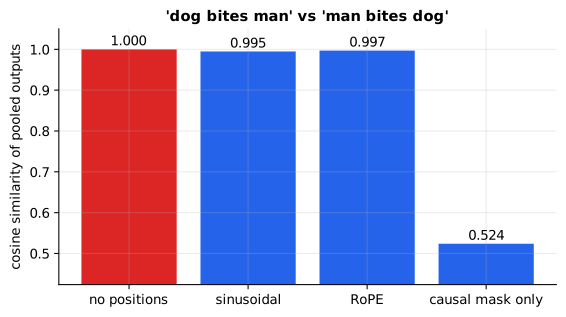
Reading it: each bar compares the pooled attention output of "dog bites man" with that of "man bites dog", as a cosine similarity (1.0 means identical). With no positions the bar reaches exactly 1: the model literally cannot tell the sentences apart. Adding sinusoidal codes or RoPE pulls the bar below 1: the sentences now look different. The causal-mask bar is below 1 too, because a mask that lets token i see only i+1 tokens already leaks some order.
In code: word_vector gives each word a fixed random embedding, and order_similarity pools each sentence's outputs and compares them, which gives the bars in the figure.
Why it matters. Almost all meaning in language is carried by order: negation scope, who did what to whom, code. So position must be injected. There are three families, below.
1. Sinusoidal codes (the original 2017 transformer)
Everyday picture. A clock with many hands. The second hand moves fast and tells nearby moments apart; the hour hand moves slowly and tells morning from evening. Read all the hands together and every moment has a unique fingerprint. Sinusoidal codes give every position such a set of "hands" and add them to the token's embedding.
Tiny worked example. With 4 dimensions there are two hands. The fast one turns 1 radian per position; the slow one turns 1/100 of a radian:
| position | sin(pos·1) | cos(pos·1) | sin(pos/100) | cos(pos/100) |
|---|---|---|---|---|
| 0 | 0.000 | 1.000 | 0.000 | 1.000 |
| 1 | 0.841 | 0.540 | 0.010 | 1.000 |
| 2 | 0.909 | −0.416 | 0.020 | 1.000 |
The fast pair already looks very different at positions 1 and 2; the slow pair barely moves, and it will only distinguish positions hundreds apart.
flowchart LR
  T["token id"] --> E["embedding lookup<br/>(what the word means)"]
  P["position 0,1,2..."] --> S["sin/cos at many frequencies<br/>(where the word is)"]
  E --> ADD(("+"))
  S --> ADD
  ADD --> B["transformer blocks"]
Reading it: two independent lookups meet at the plus sign. The top path says what the token is, the bottom path says where it is, and their sum is a single vector carrying both. Everything downstream sees only that sum, so position becomes part of the content attention compares.
The math and the code. Two functions do the work. Picture a point walking around a circle of radius 1. The angle it has turned is measured in radians (a full turn is 2π ≈ 6.28 radians). Cosine of the angle is how far right the point is, and sine is how far up; both always lie between −1 and +1, and both repeat every full turn.
Level 3: the formula and its symbols
$$ PE_{(pos,\,2i)} = \sin(pos\cdot\omega_i), \qquad PE_{(pos,\,2i+1)} = \cos(pos\cdot\omega_i), \qquad \omega_i = \frac{1}{10000^{2i/d}} $$
Symbols
| Symbol | Meaning here | In the example |
|---|---|---|
| $pos$ | the token's position, counting from 0 | 1 |
| $d$ | how many numbers each position code has | 4 |
| $i$ | which (sin, cos) pair, counting from 0 up to $d/2 - 1$ | 0 and 1 |
| $2i$, $2i+1$ | the two columns that pair $i$ fills: even column gets sine, odd gets cosine | pair 1 fills columns 2 and 3 |
| $\omega_i$ | pair $i$'s speed in radians per position (its frequency) | $\omega_0 = 1$, $\omega_1 = 1/100$ |
| $10000^{2i/d}$ | 10,000 raised to a fraction; makes each pair slower than the last | $10000^{2/4} = 100$ |
| $\sin$, $\cos$ | how far up / right a point is after turning by that many radians | $\sin 1 = 0.841$ |
| $PE_{(pos,\,c)}$ | the number in row $pos$, column $c$ of the code table |
In words: "for position pos, each pair of columns stores where a hand turning at that pair's speed points after pos steps: sine in the first column, cosine in the second."
With the numbers: d = 4, pos = 1. Pair 0 turns 1 radian: sin 1 = 0.841, cos 1 = 0.540. Pair 1 turns 1/100 radian: sin 0.01 = 0.010, cos 0.01 = 1.000. So position 1's code is (0.841, 0.540, 0.010, 1.000), the second row of the table above.
Level 3: in Python
In Python:
import math
d, pos = 4, 1
PE = []
# one (sin, cos) pair per i
for i in range(d // 2):
    # ω_i: pair i's speed
    omega_i = 1 / 10000 ** (2 * i / d)
    # columns 2i and 2i+1
    PE += [math.sin(pos * omega_i), math.cos(pos * omega_i)]
[f"{v:.3f}" for v in PE]  # → ['0.841', '0.540', '0.010', '1.000']
sinusoidal_encoding(n, d) builds the whole (n × d) table in four lines. A
shift of k positions rotates every (sin, cos) pair by the same angle k·ω_i
wherever you start, so the dot product of two position codes depends only
on their distance.
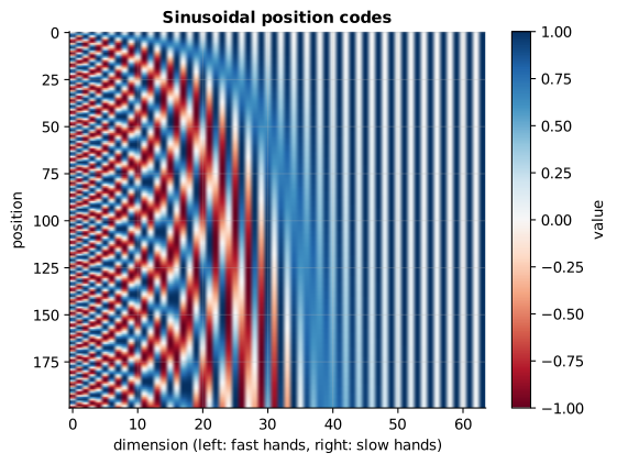
Reading it: each row is a position (0 at the top), each column one dimension, and colour is the value from −1 to +1. The left columns flip colour every few rows (fast hands); the right columns change slowly over hundreds of rows (slow hands). No two rows are identical, so every position has a unique fingerprint, and neighbouring rows look alike, so nearby positions get similar codes.
Why it matters. Fixed codes need no training and exist for any position, and the distance property lets the model learn "look 3 tokens back" once and use it everywhere. But the code is mixed into the content vector itself, which later methods avoid.
2. Learned absolute positions (GPT-2, BERT)
Everyday picture. Numbered theatre seats. Every seat has its own brass plate, and the theatre has a fixed number of seats.
Tiny worked example. GPT-2 has a table of 1,024 position vectors, each 768 numbers long: 786,432 extra parameters, learned like any other weight. Position 5 looks up row 5. Position 1,024 has no row at all.
flowchart LR
  T["token id 318"] --> TE["token table<br/>(vocab × d)"]
  P["position 5"] --> PE["position table<br/>(max_len × d)"]
  TE --> ADD(("+"))
  PE --> ADD
  ADD --> B["transformer blocks"]
  P2["position ≥ max_len"] -.-> X["no row: cannot be encoded"]
Reading it: identical to the sinusoidal picture except that the bottom path is a second trainable table instead of a formula. The dotted arrow is the catch: the table ends at max_len, so a longer input simply has nowhere to look.
The math and the code.
Level 3: the formula and its symbols
$$ x_{pos} = E_{token} + P_{pos} $$
Symbols
| Symbol | Meaning here | In the example (GPT-2) |
|---|---|---|
| $E_{token}$ | the token's row of the token table (what the word means) | 768 numbers |
| $P_{pos}$ | row $pos$ of the position table, learned during training (where it is) | 768 numbers; $pos$ from 0 to 1,023 |
| $+$ | add the two lists number by number | |
| $x_{pos}$ | the vector the first transformer block receives | 768 numbers |
In words: "the input vector is the word's meaning plus its seat number's learned vector."
With the numbers: with 2 dimensions, if $E_{dog}$ = (0.5, −0.2) and $P_{3}$ = (0.1, 0.3), then $x_3$ = (0.6, 0.1). $P_{1024}$ does not exist.
Level 3: in Python
In Python:
E_dog = [0.5, -0.2]
# a position table with rows 0 to 3
P = [[0.0, 0.0], [0.0, 0.0], [0.0, 0.0], [0.1, 0.3]]
# x_3 = E_dog + P_3
[round(e + p, 2) for e, p in zip(E_dog, P[3])]  # → [0.6, 0.1]
# no row 1024: it cannot be encoded
len(P) > 1024  # → False
primer.ml.transformer.TinyGPT uses exactly this.
Why it matters. It's simple and works well inside the trained length, but it cannot extrapolate. That limitation pushed the field to RoPE.
3. Rotary position embeddings, RoPE (Llama, Mistral, Qwen and most modern LLMs)
Everyday picture. Two people point at a clock face, one at 1 o'clock and one at 4 o'clock. The angle between their arms is 90°. Move both of them on to 8 and 11 o'clock and the angle is still 90°. RoPE turns each token's query and key like clock hands, by an amount proportional to its position. When a query meets a key, only the angle between them (the distance between the tokens) affects the score, not where on the clock they started.
Tiny worked example. Use 2 dimensions, so there is one pair turning 1 radian per position. Let q = k = (1, 0). Put the query at position 3 and the key at position 7:
- q turns by 3 rad: (cos 3, sin 3) = (−0.990, 0.141)
- k turns by 7 rad: (cos 7, sin 7) = (0.754, 0.657)
- score = −0.990·0.754 + 0.141·0.657 = −0.654 = cos(4)
Now move both 100 positions later, to 103 and 107. The score is still cos(107 − 103) = cos 4 = −0.654. Only the distance, 4, survived.
flowchart LR
  X[Token vector at position m] --> Q[q = x W_q]
  X --> K[k = x W_k]
  X --> V[v = x W_v]
  Q --> RQ["Rotate each pair of q<br/>by m·θ_i"]
  K --> RK["Rotate each pair of k<br/>by m·θ_i"]
  RQ --> S["Score = q'·k'<br/>depends only on distance"]
  RK --> S
  S --> SM[Softmax] --> W[Weighted sum of V<br/>V is NOT rotated]
  V --> W
Reading it: this is ordinary attention with one extra step on the query and key branches. After projection, each (even, odd) pair of numbers in q and k is spun like a clock hand by an angle that grows with the token's position: fast for the first pairs, slow for the last. In the dot product only the difference of the angles survives, so the score knows how far apart the tokens are but not where they sit in the document. The value branch is untouched, so what gets blended is plain content, and nothing is ever added to the embedding.
The math and the code. A rotation turns a point around the centre by some angle without changing its distance from the centre. Written as a 2 × 2 grid times a column of two numbers (a matrix-vector multiply: each output number is one row of the grid multiplied position-by-position with the input and added up):
Level 3: the formula and its symbols
$$ \begin{pmatrix} x'_{2i} \ x'_{2i+1} \end{pmatrix} = \begin{pmatrix} \cos m\theta_i & -\sin m\theta_i \ \sin m\theta_i & \cos m\theta_i \end{pmatrix} \begin{pmatrix} x_{2i} \ x_{2i+1} \end{pmatrix}, \qquad \theta_i = 10000^{-2i/d} $$
Symbols
| Symbol | Meaning here | In the example |
|---|---|---|
| $x_{2i}, x_{2i+1}$ | pair $i$ of a query or key vector, before rotating | (1, 0) |
| $x'_{2i}, x'_{2i+1}$ | the same pair after rotating | (−0.990, 0.141) |
| $m$ | the token's position | 3 |
| $i$ | which pair, from 0 to $d/2 - 1$ | 0 (the only pair when d = 2) |
| $\theta_i$ | pair $i$'s turning speed in radians per position; $10000^{-2i/d}$ means $1/10000^{2i/d}$ | $\theta_0 = 1$ |
| $m\theta_i$ | the total angle turned | 3 radians |
| the 2 × 2 grid | the rotation: row 1 gives the new first number, row 2 the new second |
In words: "new first number = cos(angle) × old first − sin(angle) × old second; new second number = sin(angle) × old first + cos(angle) × old second, where the angle is position times the pair's speed."
With the numbers: x = (1, 0) at m = 3, θ = 1: x′ = (cos 3 · 1 − sin 3 · 0, sin 3 · 1 + cos 3 · 0) = (−0.990, 0.141).
Level 3: in Python
In Python:
import math
def rotate(x, m, theta_i=1.0):
    # the angle m θ_i
    a = m * theta_i
    # row 1 of the grid
    return (math.cos(a) * x[0] - math.sin(a) * x[1],
            # row 2 of the grid
            math.sin(a) * x[0] + math.cos(a) * x[1])
[f"{v:.3f}" for v in rotate((1, 0), m=3)]  # → ['-0.990', '0.141']
d, i = 2, 0
# θ_0 = 10000^(-2i/d)
10000 ** (-2 * i / d)  # → 1.0
Why only the distance survives: turning q by angle a and k by angle b and then taking their dot product (multiply matching numbers, add them up; large when the vectors point the same way) gives the same answer as turning k alone by b − a. So
Level 3: the formula and its symbols
$$ \langle R_m q,\; R_n k\rangle = \langle q,\; R_{n-m}\, k\rangle $$
Symbols
| Symbol | Meaning here | In the example |
|---|---|---|
| $q$, $k$ | a query and a key vector, before rotating | (1, 0) and (1, 0) |
| $m$, $n$ | the query's and the key's positions | 3 and 7 |
| $R_m$ | "rotate every pair by its speed times $m$" | turn by 3 radians |
| $R_{n-m}$ | the rotation for the distance only | turn by 4 radians |
| $\langle a, b \rangle$ | the dot product of $a$ and $b$ (same as $a \cdot b$) |
In words: "the score between a query at m and a key at n equals the score you'd get by leaving the query alone and turning the key by the gap n − m."
With the numbers: left side (−0.990, 0.141) · (0.754, 0.657) = −0.654; right side (1, 0) · (cos 4, sin 4) = cos 4 = −0.654. Same number, and the same again at positions 103 and 107.
Level 3: in Python
In Python:
import math
# turn a pair by an angle (θ = 1, so the angle is the position)
def R(angle, x):
    return (math.cos(angle) * x[0] - math.sin(angle) * x[1],
            math.sin(angle) * x[0] + math.cos(angle) * x[1])
def dot(a, b): return sum(a_i * b_i for a_i, b_i in zip(a, b))
q = k = (1, 0)
# ⟨R_m q, R_n k⟩ with m = 3, n = 7
round(dot(R(3, q), R(7, k)), 3)  # → -0.654
# ⟨q, R_(n-m) k⟩: only the distance
round(dot(q, R(7 - 3, k)), 3)  # → -0.654
# 100 positions later, the same score
round(dot(R(103, q), R(107, k)), 3)  # → -0.654
apply_rope does this for a vector or a whole sequence with three
element-wise lines, and no matrix multiply.
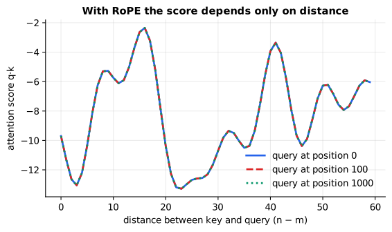
Reading it: the x-axis is the distance n − m between a query and a key; each line uses the same q and k but places the pair at a different absolute starting position (0, 100, 1,000). The lines lie exactly on top of each other: the score depends only on distance. That is the relative-position property in one picture.
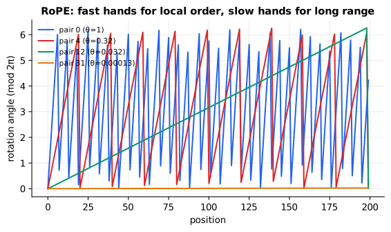
Reading it: each line is one pair of dimensions; the y-axis is how far that pair has turned (wrapped to one full turn, 2π) at each position on the x-axis. Pair 0 spins fastest and wraps every ~6 tokens, giving fine-grained local order. The last pairs barely turn across the whole range, giving coarse long-range position. It's the many-handed clock again, now applied inside attention.
In code: rope_frequencies returns each pair's turning speed θ_i, which apply_rope multiplies by the position to get every angle.
Why it matters. Relative distance is what language actually uses ("the word two back"), rotation keeps vector lengths unchanged, and because position lives in angles, you can stretch it after training. That last point is the next section.
4. Extending context after training
Everyday picture. A ruler marked from 0 to 4,000. To measure something 32,000 long you can shrink the object by 8× so it fits on the ruler (interpolation), or re-draw only the long-distance marks while keeping the fine millimetre marks (NTK-aware scaling).
Tiny worked example. A model trained on 4,096 tokens now reads 32,768. Interpolation multiplies every position by 4096/32768 = 1/8, so position 32,000 is treated as 4,000: an angle the model has seen. Neighbours are now 1/8 of a position apart, which a short fine-tune teaches it to resolve.
flowchart LR
  P["positions 0 ... 32k"] --> C{method}
  C -->|interpolation| PI["pos × 4k/32k<br/>all hands slowed 8×"]
  C -->|NTK-aware| NTK["raise the RoPE base<br/>slow hands slowed, fast hands kept"]
  PI --> R["RoPE with angles inside<br/>the trained range"]
  NTK --> R
  R --> F["short fine-tune on long text"]
Reading it: both paths solve the same problem: angles beyond what the model saw in training. Interpolation slows every hand equally, which also blurs the fast hands that encode local word order. NTK-aware scaling slows only the slow hands and leaves the fastest one untouched, so local order stays sharp. Both usually end with a brief fine-tune.
The math and the code. Position interpolation (interpolate_positions):
Level 3: the formula and its symbols
$$ pos' = pos \cdot \frac{L_{train}}{L_{new}} $$
Symbols
| Symbol | Meaning here | In the example |
|---|---|---|
| $pos$ | the real position in the long input | 32,000 |
| $L_{train}$ | the longest context seen in training | 4,096 |
| $L_{new}$ | the context we now want | 32,768 |
| $pos'$ | the position RoPE is actually given | 4,000 |
In words: "shrink every position by the ratio of old length to new length."
With the numbers: 32,000 × 4,096 / 32,768 = 32,000 / 8 = 4,000.
Level 3: in Python
In Python:
pos, L_train, L_new = 32_000, 4_096, 32_768
# pos' = pos · L_train / L_new
pos * L_train / L_new  # → 4000.0
NTK-aware scaling (ntk_scaled_base) changes the base instead:
Level 3: the formula and its symbols
$$ base' = base \cdot s^{\,d/(d-2)} $$
Symbols
| Symbol | Meaning here | In the example |
|---|---|---|
| $base$ | the 10,000 inside $\theta_i = base^{-2i/d}$ | 10,000 |
| $s$ | how many times longer the new context is | 8 |
| $d$ | the head width | 128 |
| $s^{d/(d-2)}$ | $s$ raised to a power just above 1 | $8^{1.016} ≈ 8.27$ |
| $base'$ | the new, larger base | ≈ 82,685 |
In words: "multiply the base by slightly more than the stretch factor."
With the numbers: the fastest pair keeps $\theta_0 = base'^{0} = 1$ radian per position. The slowest pair goes from $10000^{-126/128} = 1.15 \times 10^{-4}$ to $82685^{-126/128} = 1.44 \times 10^{-5}$: exactly 8× slower.
Level 3: in Python
In Python:
base, s, d = 10_000, 8, 128
# s^(d/(d-2)): just above 8
round(s ** (d / (d - 2)), 2)  # → 8.27
# base' = base · s^(d/(d-2))
base_new = base * s ** (d / (d - 2))
round(base_new)  # → 82685
# θ_i for the last pair, 2i = 126
slowest = lambda b: b ** (-126 / 128)
f"{slowest(base):.2e}", f"{slowest(base_new):.2e}"  # → ('1.15e-04', '1.44e-05')
# exactly 8× slower
round(slowest(base) / slowest(base_new), 6)  # → 8.0
YaRN refines this per frequency band and is used by many long-context models. ALiBi skips position vectors entirely and subtracts a penalty proportional to distance from each attention score.
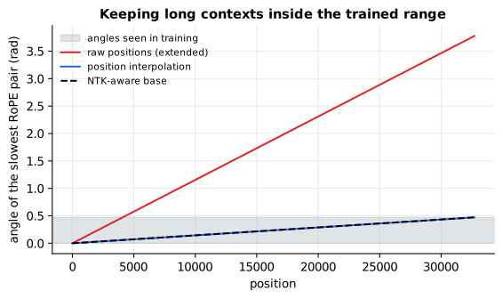
Reading it: the x-axis is position up to 32k and the y-axis is the angle of the slowest RoPE pair. The shaded band is the range of angles the model saw in training (positions up to 4k). The raw extended line leaves the band almost immediately after 4k: unfamiliar territory. The interpolated and NTK-scaled lines stay inside the band all the way to 32k.
Why it matters. It's how models trained on a few thousand tokens are cheaply stretched to 100k or more, instead of being pretrained again from scratch.
A subtlety: the causal mask leaks order
In a decoder, token i sees exactly i+1 tokens, so even with no position encoding ("NoPE") the model can partly infer where it is. Bidirectional attention (BERT-style) has no such crutch and is fully order-blind.
In code: encode_sentence with its causal flag set runs the same layer under primer.ml.attention.causal_mask; its pooled similarity is the "causal mask only" bar in the first figure.
In 20 seconds
- Attention is permutation-equivariant: shuffle the words and the outputs shuffle the same way, so without position information "dog bites man" pools to exactly the same vector as "man bites dog".
- The original transformer adds fixed sine/cosine codes; GPT-2 and BERT learn a position table that ends at max_len.
- Modern LLMs use RoPE: rotate q and k by a position-dependent angle so the score depends only on relative distance. It also makes context extension (interpolation, NTK/YaRN) practical.
Self-test questions
Why does a transformer need positional information at all? Attention compares tokens by content only, so it's permutation-equivariant: shuffling the input just shuffles the output. Without positions, word order is invisible.
How does RoPE encode position, and what property makes it attractive? It rotates each pair of dimensions in q and k by an angle proportional to position. The q·k score then depends only on the relative distance, and rotation preserves vector length.
Compute a RoPE score by hand: 2 dimensions, θ = 1, q = k = (1, 0), query at 3, key at 7. cos(7 − 3) = cos 4 ≈ −0.654, and the same at positions 103 and 107.
Why do sinusoidal codes use many frequencies? Fast frequencies distinguish neighbours; slow ones distinguish distant positions. Together every position gets a unique, smoothly varying code, and a shift by k is the same rotation everywhere.
What goes wrong beyond the trained context length, and how do you fix it? The model meets position angles or indices it never saw, and attention degrades. Position interpolation, NTK-aware scaling or YaRN rescale positions or frequencies into the trained range, usually followed by a short fine-tune.
Learned absolute position embeddings: pro and con? They are simple and effective within the trained length, but they cannot represent any position beyond the table size.
The papers behind this lesson
- Vaswani et al. (2017), Attention Is All You Need. https://arxiv.org/abs/1706.03762. Introduced the transformer and, in section 3.5, the sinusoidal position codes built here. annotated companion
- Su et al. (2021), RoFormer: Enhanced Transformer with Rotary Position Embedding. https://arxiv.org/abs/2104.09864. Introduced RoPE: rotate queries and keys so attention scores depend only on relative distance. annotated companion
- Chen et al. (2023), Extending Context Window of Large Language Models via Positional Interpolation. https://arxiv.org/abs/2306.15595. Showed that scaling positions down plus a short fine-tune extends RoPE models to much longer contexts.
- Peng et al. (2023), YaRN. https://arxiv.org/abs/2309.00071. Refined RoPE context extension by treating fast and slow frequencies differently.
- Press et al. (2021), ALiBi. https://arxiv.org/abs/2108.12409. Replaced position vectors with a distance penalty on attention scores that extrapolates to longer inputs.
Further reading
- Vaswani et al., Attention Is All You Need (sinusoidal codes, section 3.5): https://arxiv.org/abs/1706.03762
- Su et al., RoFormer: Enhanced Transformer with Rotary Position Embedding (2021): https://arxiv.org/abs/2104.09864
- EleutherAI, Rotary Embeddings: A Relative Revolution: https://blog.eleuther.ai/rotary-embeddings/
- Chen et al., Extending Context Window of Large Language Models via Positional Interpolation (2023): https://arxiv.org/abs/2306.15595
- Peng et al., YaRN: Efficient Context Window Extension of Large Language Models (2023): https://arxiv.org/abs/2309.00071
- Press et al., Train Short, Test Long: Attention with Linear Biases (ALiBi) (2021): https://arxiv.org/abs/2108.12409
- Kazemnejad et al., The Impact of Positional Encoding on Length Generalization in Transformers (NoPE, 2023): https://arxiv.org/abs/2305.19466
1r""" 2# Positional information: how a transformer knows word order 3 4Run: `python -m primer.ml.positional` 5 6New to the notation (vectors, dot products, sine and cosine)? Every symbol 7is decoded where it appears, and `primer.notation` teaches them all from zero. 8This lesson builds on `primer.ml.attention`. 9 10## Level 1: The practitioner's guide 11 12**In one sentence.** Positional encoding is how a transformer learns where 13each token sits, since attention on its own treats the input as an unordered 14bag; the scheme a model uses decides how long a context it can read, whether 15that length can be stretched after training, and what happens when you go 16past it. 17 18**When you need it.** You never add positions yourself; the model's authors 19chose a scheme before training and it is baked into the weights. You meet it 20the day a length matters: a model card says 128K tokens and you wonder how 21far to trust it, a self-hosted model produces nonsense past a certain prompt 22length, an embedding model rejects documents longer than its limit, or you 23want to fine-tune a model to read documents longer than it was trained on. 24The tell: quality that is fine at 4,000 tokens and falls off a cliff at 25some longer length, with nothing in the logs. The number behind the whole 26topic, from this lesson's `order_similarity`: with no positions, the pooled 27attention outputs for "dog bites man" and "man bites dog" have cosine 28similarity exactly 1.000. The model cannot tell them apart. Nothing about 29this concerns you when prompts stay well inside the length the model was 30trained at. 31 32**Your options.** The first four are choices the model's authors made; you 33choose among them by choosing a model. The last three are what you or the 34vendor can do about length afterwards. From the simplest to the most 35committed: 36 37| Option | What it does | What it gives you | What it costs | Where it lives | 38|---|---|---|---|---| 39| A learned position table (GPT-2, BERT) | One learned vector per seat, added to the token's vector | Simple and effective inside the trained length | A hard ceiling: no row exists past the table's end (1,024 rows for GPT-2, 512 for BERT) | The architecture; `max_position_embeddings` on the card | 40| Sinusoidal codes (the 2017 transformer) | A fixed sine and cosine fingerprint per position, added to the token | No parameters; a code exists for any position | Position is mixed into content; little used in new models | The architecture | 41| RoPE (Llama, Mistral, Qwen) | Rotates each query and key by an angle that grows with position, so scores depend on the distance between tokens | Relative distance for free, and a context that can be stretched after training | Angles past the trained range are unfamiliar; extension needs scaling | The architecture; `rope_theta` and `rope_parameters` on the card | 42| ALiBi | Subtracts a penalty proportional to distance from each score; no position vectors at all | Trained at 1,024 tokens, it extrapolates to 2,048; 11% faster and 11% less memory than sinusoidal in its paper | A built-in preference for nearby tokens; fewer models use it | The architecture | 43| Inference-time scaling (linear or dynamic NTK) | Rescales positions or the RoPE base: linear scaling at every length, dynamic scaling only once a prompt exceeds the trained length | A modest stretch with no training at all | Quality drops as the stretch grows | The serving engine's config: `rope_type` and `factor` | 44| Extension with a short fine-tune (PI, YaRN) | Scales positions into the trained range, then fine-tunes briefly on long text | 8× longer context: Llama to 32,768 tokens within 1,000 steps (PI); YaRN needs 10× fewer tokens than earlier methods | Long documents to train on, a training run, an evaluation at length | Your training stack | 45| Staged long-context pretraining | The vendor grows the window during pretraining, checking a needle-in-a-haystack test at each stage | The genuine article: Llama 3 went from 8K to 128K in six stages | About 800B training tokens for Llama 3 405B; reaches you as a number on the card | The vendor | 46 47**How to choose.** Start from the model in front of you. 48 49- A hosted API: nothing to choose, but the window on the card is the length 50 the vendor trained and tested, not a promise about your task. Measure at 51 the lengths you will use. 52- Picking an open model: read `max_position_embeddings` and 53 `rope_parameters`. An entry with a `factor` means the model was trained 54 shorter and stretched, so test it at the lengths you will use rather 55 than trusting the stretched number. 56- Serving a model beyond its trained length: do not raise the engine's 57 context limit on its own. Set the scaling the checkpoint expects (or a 58 dynamic scaling if none is given), and test before shipping. 59- Documents longer than the model's window, and you can train: position 60 interpolation or YaRN plus a fine-tune on long text, with a 61 needle-in-a-haystack check and your own task at the target length. 62- An encoder or embedding model with a learned table: the limit is hard. 63 Chunk documents to fit (`primer.agents.rag`). 64- Whatever you pick, evaluate at the length you will run, with the answer 65 placed at the start, the middle and the end of the prompt. 66 67**What it costs.** Positions are nearly free to compute; length is what 68costs. 69 70- Parameters and compute. GPT-2's table is 1,024 × 768 = 786,432 numbers, 71 under 1% of its 124 million parameters. RoPE and ALiBi add none, and RoPE 72 is a few element-wise multiplications per query and key, negligible next 73 to attention itself. 74- Stretching. Position interpolation for 4,096 to 32,768 tokens multiplies 75 every position by 1/8 (32,000 becomes 4,000); NTK-aware scaling instead 76 raises the RoPE base from 10,000 to 82,685 for a 128-wide head, leaving 77 the fastest pair untouched and slowing the slowest 8×. Both are followed 78 by a short fine-tune: within 1,000 steps in the PI paper. Llama 3's 79 authors set the base to 500,000 and spent about 800B tokens taking the 80 405B model from 8K to 128K. 81- Quality. RoPE gives nearby tokens a head start (the RoFormer companion's 82 long-term decay), and a long window is not used evenly: Liu et al. (*Lost 83 in the Middle*, 2023) found models use information best at the start or 84 the end of a long prompt and worst in the middle (`primer.agents.context`). 85 86**What breaks.** 87 88- **Past the table.** A learned-table model has no vector for position 89 1,024 if its table has 1,024 rows: the request fails or the library 90 truncates. Chunk the input. 91- **Past the trained angles.** RoPE degrades silently rather than failing: 92 this lesson's figure shows the slowest pair's angle leaving the trained 93 band right after 4K tokens and reaching 8× its top by 32K. The PI paper 94 reports that plain extrapolation can produce catastrophically large 95 attention scores. Scale, then fine-tune. 96- **A checkpoint served with the wrong scaling.** An extended model whose 97 `rope_parameters` are dropped or mistyped reads positions it never 98 learned. Copy the config with the weights. 99- **Interpolating too far.** Interpolation slows every frequency equally, 100 which also blurs the fast ones that carry local word order. NTK-aware 101 scaling and YaRN keep the fast frequencies, which is why they are 102 preferred for large stretches. 103- **Pooling that forgets order.** Average the token vectors of an 104 order-blind model and "dog bites man" equals "man bites dog" exactly. 105 Order survives only if positions are injected, or an encoding step that 106 is not permutation-blind comes first. 107- **Trusting the causal mask for order.** In a decoder the mask alone lets 108 the sentences differ (cosine 0.524 in this lesson's run), but it is a 109 weak signal, not a position encoding. 110 111**In the wild.** The original transformer (Vaswani et al., 2017) used 112sinusoidal codes; GPT-2 and BERT switched to learned tables, which is why 113each has a fixed maximum length. Llama, Mistral and Qwen use RoPE, and Llama 1143 raised its base to 500,000 with 8 key-value heads beside it. Hugging Face 115model configs carry the scheme as `rope_parameters` with a `rope_type` of 116`linear`, `dynamic`, `yarn`, `longrope` or `llama3`, a `factor` and an 117`original_max_position_embeddings`; vLLM's `--max-model-len` sets the 118served length and `--hf-overrides` changes that config at load time. YaRN 119(Peng et al., 2023) is the extension recipe behind many long-context 120checkpoints, ALiBi (Press et al., 2021) the alternative that extrapolates 121without vectors, and the NoPE study (Kazemnejad et al., 2023) found that a 122decoder can generalize to longer inputs with no explicit positions at all. 123The papers are linked at the end of the lesson. 124 125**Go deeper.** Level 2 shows the bag-of-words problem in three numbers, 126builds sinusoidal codes as a clock with many hands, checks RoPE's distance 127property by hand at positions 3 and 7 and again at 103 and 107, and stretches 128a 4K model to 32K by interpolation and by raising the base. If you only 129needed to read a model card or serve a model safely, you are done. 130 131## Level 2: How it works, from scratch 132 133Level 2 starts with the problem itself, a bag of Scrabble tiles, and adds 134each family of positions in turn. 135 136## The problem: attention reads a bag, not a sentence 137 138**Everyday picture.** Pour the words of a sentence into a bag of Scrabble 139tiles. The bag for "dog bites man" and the bag for "man bites dog" hold 140exactly the same tiles. Anyone who only gets the bag cannot tell a news 141story from a routine dog attack. Attention, on its own, only ever gets the bag. 142 143**Tiny worked example.** Give each word a 2-number embedding: dog = (1, 0), 144bites = (0, 1), man = (1, 1). Average the words of each sentence, which is 145the simplest possible "sentence vector": 146 147| sentence | sum of vectors | average | 148|---|---|---| 149| dog bites man | (1,0)+(0,1)+(1,1) = (2, 2) | (0.67, 0.67) | 150| man bites dog | (1,1)+(0,1)+(1,0) = (2, 2) | (0.67, 0.67) | 151 152Addition doesn't care about order, and neither does attention: every token 153compares itself with every other by dot product, and nothing in that 154computation says who came first. 155 156```mermaid 157flowchart LR 158 A["'dog bites man'"] --> E1[Embed each token] 159 B["'man bites dog'"] --> E2[Embed each token] 160 E1 --> S1["Set {dog, bites, man}"] 161 E2 --> S2["Set {man, bites, dog}"] 162 S1 --> ATT[Attention with no positions] 163 S2 --> ATT 164 ATT --> SAME[Same vectors, only reordered:<br/>the meaning difference is lost] 165``` 166 167**Reading it:** follow both sentences left to right. Embedding looks up each 168token independently, so both sentences produce the same three vectors. 169Attention only compares vectors with each other; it has no notion of slot 1 170versus slot 3. It sees the same *set* and produces the same output vectors, 171listed in a different order. Pool them into one sentence vector and the two 172sentences are identical. 173 174**The math.** A **permutation** is a reshuffle of an ordered list. Written as 175a matrix (a grid of numbers), a permutation matrix is all zeros except one 1 176in each row, and multiplying by it just reorders rows. Attention without 177positions is *permutation-equivariant*: 178 179$$ 180\text{Attn}(PX) = P\,\text{Attn}(X) 181$$ 182 183**Symbols** 184 185| Symbol | Meaning here | In the example | 186|---|---|---| 187| $X$ | the sentence's token vectors, one row per word | rows dog (1,0), bites (0,1), man (1,1): a 3 × 2 grid | 188| $P$ | a permutation matrix: reorders the rows of whatever it multiplies | swap rows 1 and 3 | 189| $PX$ | the same rows in the new order | man (1,1), bites (0,1), dog (1,0) | 190| $\text{Attn}(\cdot)$ | one attention layer with no position information (here with $W_q = W_k = W_v$ = identity, so q = k = v = the word vector) | 3 × 2 in, 3 × 2 out | 191| $=$ | both sides are exactly the same grid of numbers | | 192 193**In words:** "running attention on the shuffled sentence gives the same 194answer as running it on the original sentence and shuffling afterwards." 195 196**With the numbers:** in "dog bites man", dog's query (1,0) scores the three 197keys (1,0), (0,1), (1,1) as 1, 0, 1; divided by √2 that is 0.707, 0, 0.707. 198Softmax gives weights 0.401, 0.198, 0.401, so dog's output is 1990.401·(1,0) + 0.198·(0,1) + 0.401·(1,1) = **(0.802, 0.599)**. In "man bites 200dog" dog sits in row 3, but it scores the same three keys in a different 201order, gets the same weights, and outputs the same **(0.802, 0.599)**. 202 203**In Python:** 204 205```python 206import math 207# q = k = v = the word vector, no positions 208def Attn(X): 209 out = [] 210 for q in X: 211 scores = [sum(a * b for a, b in zip(q, k)) / math.sqrt(2) for k in X] 212 exps = [math.exp(s) for s in scores] 213 weights = [e / sum(exps) for e in exps] 214 out.append(tuple(round(sum(w * v[c] for w, v in zip(weights, X)), 3) for c in range(2))) 215 return out 216# dog, bites, man 217X = [(1, 0), (0, 1), (1, 1)] 218# P swaps rows 1 and 3: man, bites, dog 219PX = [X[2], X[1], X[0]] 220Attn(X) # → [(0.802, 0.599), (0.599, 0.802), (0.752, 0.752)] 221# the same rows, shuffled the same way 222Attn(PX) # → [(0.752, 0.752), (0.599, 0.802), (0.802, 0.599)] 223``` 224 225Shuffle the input and you get the same outputs, shuffled the same way. 226`encode_sentence(..., scheme="none")` runs a real attention layer and shows 227the "dog" row is the same vector whether "dog" comes first or last. 228 229 230 231**Reading it:** each bar compares the pooled attention output of "dog bites 232man" with that of "man bites dog", as a cosine similarity (1.0 means 233identical). With no positions the bar reaches exactly 1: the model literally 234cannot tell the sentences apart. Adding sinusoidal codes or RoPE pulls the 235bar below 1: the sentences now look different. The causal-mask bar is below 1 236too, because a mask that lets token i see only i+1 tokens already leaks some 237order. 238 239**In code:** `word_vector` gives each word a fixed random embedding, and `order_similarity` pools each sentence's outputs and compares them, which gives the bars in the figure. 240 241**Why it matters.** Almost all meaning in language is carried by order: 242negation scope, who did what to whom, code. So position must be **injected**. 243There are three families, below. 244 245## 1. Sinusoidal codes (the original 2017 transformer) 246 247**Everyday picture.** A clock with many hands. The second hand moves fast 248and tells nearby moments apart; the hour hand moves slowly and tells morning 249from evening. Read all the hands together and every moment has a unique 250fingerprint. Sinusoidal codes give every position such a set of "hands" and 251add them to the token's embedding. 252 253**Tiny worked example.** With 4 dimensions there are two hands. The fast one 254turns 1 radian per position; the slow one turns 1/100 of a radian: 255 256| position | sin(pos·1) | cos(pos·1) | sin(pos/100) | cos(pos/100) | 257|---|---|---|---|---| 258| 0 | 0.000 | 1.000 | 0.000 | 1.000 | 259| 1 | 0.841 | 0.540 | 0.010 | 1.000 | 260| 2 | 0.909 | −0.416 | 0.020 | 1.000 | 261 262The fast pair already looks very different at positions 1 and 2; the slow 263pair barely moves, and it will only distinguish positions hundreds apart. 264 265```mermaid 266flowchart LR 267 T["token id"] --> E["embedding lookup<br/>(what the word means)"] 268 P["position 0,1,2..."] --> S["sin/cos at many frequencies<br/>(where the word is)"] 269 E --> ADD(("+")) 270 S --> ADD 271 ADD --> B["transformer blocks"] 272``` 273 274**Reading it:** two independent lookups meet at the plus sign. The top path 275says *what* the token is, the bottom path says *where* it is, and their sum 276is a single vector carrying both. Everything downstream sees only that sum, 277so position becomes part of the content attention compares. 278 279**The math and the code.** Two functions do the work. Picture a point 280walking around a circle of radius 1. The angle it has turned is measured in 281**radians** (a full turn is 2π ≈ 6.28 radians). **Cosine** of the angle is 282how far right the point is, and **sine** is how far up; both always lie 283between −1 and +1, and both repeat every full turn. 284 285$$ 286PE_{(pos,\,2i)} = \sin(pos\cdot\omega_i), \qquad PE_{(pos,\,2i+1)} = \cos(pos\cdot\omega_i), 287\qquad \omega_i = \frac{1}{10000^{2i/d}} 288$$ 289 290**Symbols** 291 292| Symbol | Meaning here | In the example | 293|---|---|---| 294| $pos$ | the token's position, counting from 0 | 1 | 295| $d$ | how many numbers each position code has | 4 | 296| $i$ | which (sin, cos) pair, counting from 0 up to $d/2 - 1$ | 0 and 1 | 297| $2i$, $2i+1$ | the two columns that pair $i$ fills: even column gets sine, odd gets cosine | pair 1 fills columns 2 and 3 | 298| $\omega_i$ | pair $i$'s speed in radians per position (its **frequency**) | $\omega_0 = 1$, $\omega_1 = 1/100$ | 299| $10000^{2i/d}$ | 10,000 raised to a fraction; makes each pair slower than the last | $10000^{2/4} = 100$ | 300| $\sin$, $\cos$ | how far up / right a point is after turning by that many radians | $\sin 1 = 0.841$ | 301| $PE_{(pos,\,c)}$ | the number in row $pos$, column $c$ of the code table | | 302 303**In words:** "for position *pos*, each pair of columns stores where a hand 304turning at that pair's speed points after *pos* steps: sine in the first 305column, cosine in the second." 306 307**With the numbers:** d = 4, pos = 1. Pair 0 turns 1 radian: sin 1 = 0.841, 308cos 1 = 0.540. Pair 1 turns 1/100 radian: sin 0.01 = 0.010, cos 0.01 = 1.000. 309So position 1's code is **(0.841, 0.540, 0.010, 1.000)**, the second row of 310the table above. 311 312**In Python:** 313 314```python 315import math 316d, pos = 4, 1 317PE = [] 318# one (sin, cos) pair per i 319for i in range(d // 2): 320 # ω_i: pair i's speed 321 omega_i = 1 / 10000 ** (2 * i / d) 322 # columns 2i and 2i+1 323 PE += [math.sin(pos * omega_i), math.cos(pos * omega_i)] 324[f"{v:.3f}" for v in PE] # → ['0.841', '0.540', '0.010', '1.000'] 325``` 326 327`sinusoidal_encoding(n, d)` builds the whole (n × d) table in four lines. A 328shift of k positions rotates every (sin, cos) pair by the same angle k·ω_i 329wherever you start, so **the dot product of two position codes depends only 330on their distance**. 331 332 333 334**Reading it:** each row is a position (0 at the top), each column one 335dimension, and colour is the value from −1 to +1. The left columns flip 336colour every few rows (fast hands); the right columns change slowly over 337hundreds of rows (slow hands). No two rows are identical, so every position 338has a unique fingerprint, and neighbouring rows look alike, so nearby 339positions get similar codes. 340 341**Why it matters.** Fixed codes need no training and exist for any position, 342and the distance property lets the model learn "look 3 tokens back" once and 343use it everywhere. But the code is mixed into the content vector itself, 344which later methods avoid. 345 346## 2. Learned absolute positions (GPT-2, BERT) 347 348**Everyday picture.** Numbered theatre seats. Every seat has its own brass 349plate, and the theatre has a fixed number of seats. 350 351**Tiny worked example.** GPT-2 has a table of 1,024 position vectors, each 352768 numbers long: 786,432 extra parameters, learned like any other weight. 353Position 5 looks up row 5. Position 1,024 has no row at all. 354 355```mermaid 356flowchart LR 357 T["token id 318"] --> TE["token table<br/>(vocab × d)"] 358 P["position 5"] --> PE["position table<br/>(max_len × d)"] 359 TE --> ADD(("+")) 360 PE --> ADD 361 ADD --> B["transformer blocks"] 362 P2["position ≥ max_len"] -.-> X["no row: cannot be encoded"] 363``` 364 365**Reading it:** identical to the sinusoidal picture except that the bottom 366path is a second trainable table instead of a formula. The dotted arrow is 367the catch: the table ends at max_len, so a longer input simply has nowhere 368to look. 369 370**The math and the code.** 371 372$$ 373x_{pos} = E_{token} + P_{pos} 374$$ 375 376**Symbols** 377 378| Symbol | Meaning here | In the example (GPT-2) | 379|---|---|---| 380| $E_{token}$ | the token's row of the token table (what the word means) | 768 numbers | 381| $P_{pos}$ | row $pos$ of the position table, learned during training (where it is) | 768 numbers; $pos$ from 0 to 1,023 | 382| $+$ | add the two lists number by number | | 383| $x_{pos}$ | the vector the first transformer block receives | 768 numbers | 384 385**In words:** "the input vector is the word's meaning plus its seat number's 386learned vector." 387 388**With the numbers:** with 2 dimensions, if $E_{dog}$ = (0.5, −0.2) and 389$P_{3}$ = (0.1, 0.3), then $x_3$ = (0.6, 0.1). $P_{1024}$ does not exist. 390 391**In Python:** 392 393```python 394E_dog = [0.5, -0.2] 395# a position table with rows 0 to 3 396P = [[0.0, 0.0], [0.0, 0.0], [0.0, 0.0], [0.1, 0.3]] 397# x_3 = E_dog + P_3 398[round(e + p, 2) for e, p in zip(E_dog, P[3])] # → [0.6, 0.1] 399# no row 1024: it cannot be encoded 400len(P) > 1024 # → False 401``` 402 403`primer.ml.transformer.TinyGPT` uses exactly this. 404 405**Why it matters.** It's simple and works well inside the trained length, 406but it cannot extrapolate. That limitation pushed the field to RoPE. 407 408## 3. Rotary position embeddings, RoPE (Llama, Mistral, Qwen and most modern LLMs) 409 410**Everyday picture.** Two people point at a clock face, one at 1 o'clock and 411one at 4 o'clock. The angle between their arms is 90°. Move both of them on 412to 8 and 11 o'clock and the angle is still 90°. RoPE turns each token's 413query and key like clock hands, by an amount proportional to its position. 414When a query meets a key, only the **angle between them** (the distance 415between the tokens) affects the score, not where on the clock they started. 416 417**Tiny worked example.** Use 2 dimensions, so there is one pair turning 1 418radian per position. Let q = k = (1, 0). Put the query at position 3 and the 419key at position 7: 420 421* q turns by 3 rad: (cos 3, sin 3) = (−0.990, 0.141) 422* k turns by 7 rad: (cos 7, sin 7) = (0.754, 0.657) 423* score = −0.990·0.754 + 0.141·0.657 = −0.654 = cos(4) 424 425Now move both 100 positions later, to 103 and 107. The score is still 426cos(107 − 103) = cos 4 = −0.654. Only the distance, 4, survived. 427 428```mermaid 429flowchart LR 430 X[Token vector at position m] --> Q[q = x W_q] 431 X --> K[k = x W_k] 432 X --> V[v = x W_v] 433 Q --> RQ["Rotate each pair of q<br/>by m·θ_i"] 434 K --> RK["Rotate each pair of k<br/>by m·θ_i"] 435 RQ --> S["Score = q'·k'<br/>depends only on distance"] 436 RK --> S 437 S --> SM[Softmax] --> W[Weighted sum of V<br/>V is NOT rotated] 438 V --> W 439``` 440 441**Reading it:** this is ordinary attention with one extra step on the query 442and key branches. After projection, each (even, odd) pair of numbers in q 443and k is spun like a clock hand by an angle that grows with the token's 444position: fast for the first pairs, slow for the last. In the dot product 445only the *difference* of the angles survives, so the score knows how far 446apart the tokens are but not where they sit in the document. The value 447branch is untouched, so what gets blended is plain content, and nothing is 448ever added to the embedding. 449 450**The math and the code.** A **rotation** turns a point around the centre 451by some angle without changing its distance from the centre. Written as a 4522 × 2 grid times a column of two numbers (a **matrix-vector multiply**: 453each output number is one row of the grid multiplied position-by-position 454with the input and added up): 455 456$$ 457\begin{pmatrix} x'_{2i} \\ x'_{2i+1} \end{pmatrix} = 458\begin{pmatrix} \cos m\theta_i & -\sin m\theta_i \\ \sin m\theta_i & \cos m\theta_i \end{pmatrix} 459\begin{pmatrix} x_{2i} \\ x_{2i+1} \end{pmatrix}, 460\qquad \theta_i = 10000^{-2i/d} 461$$ 462 463**Symbols** 464 465| Symbol | Meaning here | In the example | 466|---|---|---| 467| $x_{2i}, x_{2i+1}$ | pair $i$ of a query or key vector, before rotating | (1, 0) | 468| $x'_{2i}, x'_{2i+1}$ | the same pair after rotating | (−0.990, 0.141) | 469| $m$ | the token's position | 3 | 470| $i$ | which pair, from 0 to $d/2 - 1$ | 0 (the only pair when d = 2) | 471| $\theta_i$ | pair $i$'s turning speed in radians per position; $10000^{-2i/d}$ means $1/10000^{2i/d}$ | $\theta_0 = 1$ | 472| $m\theta_i$ | the total angle turned | 3 radians | 473| the 2 × 2 grid | the rotation: row 1 gives the new first number, row 2 the new second | | 474 475**In words:** "new first number = cos(angle) × old first − sin(angle) × old 476second; new second number = sin(angle) × old first + cos(angle) × old second, 477where the angle is position times the pair's speed." 478 479**With the numbers:** x = (1, 0) at m = 3, θ = 1: x′ = (cos 3 · 1 − sin 3 · 0, 480sin 3 · 1 + cos 3 · 0) = (−0.990, 0.141). 481 482**In Python:** 483 484```python 485import math 486def rotate(x, m, theta_i=1.0): 487 # the angle m θ_i 488 a = m * theta_i 489 # row 1 of the grid 490 return (math.cos(a) * x[0] - math.sin(a) * x[1], 491 # row 2 of the grid 492 math.sin(a) * x[0] + math.cos(a) * x[1]) 493[f"{v:.3f}" for v in rotate((1, 0), m=3)] # → ['-0.990', '0.141'] 494d, i = 2, 0 495# θ_0 = 10000^(-2i/d) 49610000 ** (-2 * i / d) # → 1.0 497``` 498 499Why only the distance survives: turning q by angle a and k by angle b and 500then taking their **dot product** (multiply matching numbers, add them up; 501large when the vectors point the same way) gives the same answer as turning 502k alone by b − a. So 503 504$$ 505\langle R_m q,\; R_n k\rangle = \langle q,\; R_{n-m}\, k\rangle 506$$ 507 508**Symbols** 509 510| Symbol | Meaning here | In the example | 511|---|---|---| 512| $q$, $k$ | a query and a key vector, before rotating | (1, 0) and (1, 0) | 513| $m$, $n$ | the query's and the key's positions | 3 and 7 | 514| $R_m$ | "rotate every pair by its speed times $m$" | turn by 3 radians | 515| $R_{n-m}$ | the rotation for the *distance* only | turn by 4 radians | 516| $\langle a, b \rangle$ | the dot product of $a$ and $b$ (same as $a \cdot b$) | | 517 518**In words:** "the score between a query at *m* and a key at *n* equals the 519score you'd get by leaving the query alone and turning the key by the gap 520*n − m*." 521 522**With the numbers:** left side (−0.990, 0.141) · (0.754, 0.657) = −0.654; 523right side (1, 0) · (cos 4, sin 4) = cos 4 = −0.654. Same number, and the same 524again at positions 103 and 107. 525 526**In Python:** 527 528```python 529import math 530# turn a pair by an angle (θ = 1, so the angle is the position) 531def R(angle, x): 532 return (math.cos(angle) * x[0] - math.sin(angle) * x[1], 533 math.sin(angle) * x[0] + math.cos(angle) * x[1]) 534def dot(a, b): return sum(a_i * b_i for a_i, b_i in zip(a, b)) 535q = k = (1, 0) 536# ⟨R_m q, R_n k⟩ with m = 3, n = 7 537round(dot(R(3, q), R(7, k)), 3) # → -0.654 538# ⟨q, R_(n-m) k⟩: only the distance 539round(dot(q, R(7 - 3, k)), 3) # → -0.654 540# 100 positions later, the same score 541round(dot(R(103, q), R(107, k)), 3) # → -0.654 542``` 543 544`apply_rope` does this for a vector or a whole sequence with three 545element-wise lines, and no matrix multiply. 546 547 548 549**Reading it:** the x-axis is the distance n − m between a query and a key; 550each line uses the same q and k but places the pair at a different absolute 551starting position (0, 100, 1,000). The lines lie exactly on top of each 552other: the score depends only on distance. That is the relative-position 553property in one picture. 554 555 556 557**Reading it:** each line is one pair of dimensions; the y-axis is how far 558that pair has turned (wrapped to one full turn, 2π) at each position on the 559x-axis. Pair 0 spins fastest and wraps every ~6 tokens, giving fine-grained 560local order. The last pairs barely turn across the whole range, giving 561coarse long-range position. It's the many-handed clock again, now applied 562inside attention. 563 564**In code:** `rope_frequencies` returns each pair's turning speed θ_i, which `apply_rope` multiplies by the position to get every angle. 565 566**Why it matters.** Relative distance is what language actually uses ("the 567word two back"), rotation keeps vector lengths unchanged, and because 568position lives in angles, you can stretch it after training. That last 569point is the next section. 570 571## 4. Extending context after training 572 573**Everyday picture.** A ruler marked from 0 to 4,000. To measure something 57432,000 long you can shrink the object by 8× so it fits on the ruler 575(interpolation), or re-draw only the long-distance marks while keeping the 576fine millimetre marks (NTK-aware scaling). 577 578**Tiny worked example.** A model trained on 4,096 tokens now reads 32,768. 579Interpolation multiplies every position by 4096/32768 = 1/8, so position 58032,000 is treated as 4,000: an angle the model has seen. Neighbours are now 5811/8 of a position apart, which a short fine-tune teaches it to resolve. 582 583```mermaid 584flowchart LR 585 P["positions 0 ... 32k"] --> C{method} 586 C -->|interpolation| PI["pos × 4k/32k<br/>all hands slowed 8×"] 587 C -->|NTK-aware| NTK["raise the RoPE base<br/>slow hands slowed, fast hands kept"] 588 PI --> R["RoPE with angles inside<br/>the trained range"] 589 NTK --> R 590 R --> F["short fine-tune on long text"] 591``` 592 593**Reading it:** both paths solve the same problem: angles beyond what the 594model saw in training. Interpolation slows *every* hand equally, which also 595blurs the fast hands that encode local word order. NTK-aware scaling slows 596only the slow hands and leaves the fastest one untouched, so local order stays 597sharp. Both usually end with a brief fine-tune. 598 599**The math and the code.** Position interpolation (`interpolate_positions`): 600 601$$ 602pos' = pos \cdot \frac{L_{train}}{L_{new}} 603$$ 604 605**Symbols** 606 607| Symbol | Meaning here | In the example | 608|---|---|---| 609| $pos$ | the real position in the long input | 32,000 | 610| $L_{train}$ | the longest context seen in training | 4,096 | 611| $L_{new}$ | the context we now want | 32,768 | 612| $pos'$ | the position RoPE is actually given | 4,000 | 613 614**In words:** "shrink every position by the ratio of old length to new length." 615 616**With the numbers:** 32,000 × 4,096 / 32,768 = 32,000 / 8 = **4,000**. 617 618**In Python:** 619 620```python 621pos, L_train, L_new = 32_000, 4_096, 32_768 622# pos' = pos · L_train / L_new 623pos * L_train / L_new # → 4000.0 624``` 625 626NTK-aware scaling (`ntk_scaled_base`) changes the base instead: 627 628$$ 629base' = base \cdot s^{\,d/(d-2)} 630$$ 631 632**Symbols** 633 634| Symbol | Meaning here | In the example | 635|---|---|---| 636| $base$ | the 10,000 inside $\theta_i = base^{-2i/d}$ | 10,000 | 637| $s$ | how many times longer the new context is | 8 | 638| $d$ | the head width | 128 | 639| $s^{d/(d-2)}$ | $s$ raised to a power just above 1 | $8^{1.016} ≈ 8.27$ | 640| $base'$ | the new, larger base | ≈ 82,685 | 641 642**In words:** "multiply the base by slightly more than the stretch factor." 643 644**With the numbers:** the fastest pair keeps $\theta_0 = base'^{0} = 1$ 645radian per position. The slowest pair goes from $10000^{-126/128} = 1.15 646\times 10^{-4}$ to $82685^{-126/128} = 1.44 \times 10^{-5}$: exactly 8× slower. 647 648**In Python:** 649 650```python 651base, s, d = 10_000, 8, 128 652# s^(d/(d-2)): just above 8 653round(s ** (d / (d - 2)), 2) # → 8.27 654# base' = base · s^(d/(d-2)) 655base_new = base * s ** (d / (d - 2)) 656round(base_new) # → 82685 657# θ_i for the last pair, 2i = 126 658slowest = lambda b: b ** (-126 / 128) 659f"{slowest(base):.2e}", f"{slowest(base_new):.2e}" # → ('1.15e-04', '1.44e-05') 660# exactly 8× slower 661round(slowest(base) / slowest(base_new), 6) # → 8.0 662``` 663 664YaRN refines this per frequency band and is 665used by many long-context models. ALiBi skips position vectors entirely and 666subtracts a penalty proportional to distance from each attention score. 667 668 669 670**Reading it:** the x-axis is position up to 32k and the y-axis is the angle 671of the slowest RoPE pair. The shaded band is the range of angles the model 672saw in training (positions up to 4k). The raw extended line leaves the band 673almost immediately after 4k: unfamiliar territory. The interpolated and 674NTK-scaled lines stay inside the band all the way to 32k. 675 676**Why it matters.** It's how models trained on a few thousand tokens are 677cheaply stretched to 100k or more, instead of being pretrained again from 678scratch. 679 680## A subtlety: the causal mask leaks order 681 682In a decoder, token i sees exactly i+1 tokens, so even with no position 683encoding ("NoPE") the model can partly infer where it is. Bidirectional 684attention (BERT-style) has no such crutch and is fully order-blind. 685 686**In code:** `encode_sentence` with its causal flag set runs the same layer under `primer.ml.attention.causal_mask`; its pooled similarity is the "causal mask only" bar in the first figure. 687 688## In 20 seconds 689- Attention is permutation-equivariant: shuffle the words and the outputs 690 shuffle the same way, so without position information "dog bites man" 691 pools to exactly the same vector as "man bites dog". 692- The original transformer adds fixed sine/cosine codes; GPT-2 and BERT 693 learn a position table that ends at max_len. 694- Modern LLMs use RoPE: rotate q and k by a position-dependent angle so the 695 score depends only on relative distance. It also makes context extension 696 (interpolation, NTK/YaRN) practical. 697 698## Self-test questions 699 700**Why does a transformer need positional information at all?** 701Attention compares tokens by content only, so it's permutation-equivariant: 702shuffling the input just shuffles the output. Without positions, word order 703is invisible. 704 705**How does RoPE encode position, and what property makes it attractive?** 706It rotates each pair of dimensions in q and k by an angle proportional to 707position. The q·k score then depends only on the relative distance, and 708rotation preserves vector length. 709 710**Compute a RoPE score by hand: 2 dimensions, θ = 1, q = k = (1, 0), query at 3, key at 7.** 711cos(7 − 3) = cos 4 ≈ −0.654, and the same at positions 103 and 107. 712 713**Why do sinusoidal codes use many frequencies?** 714Fast frequencies distinguish neighbours; slow ones distinguish distant 715positions. Together every position gets a unique, smoothly varying code, and 716a shift by k is the same rotation everywhere. 717 718**What goes wrong beyond the trained context length, and how do you fix it?** 719The model meets position angles or indices it never saw, and attention 720degrades. Position interpolation, NTK-aware scaling or YaRN rescale positions 721or frequencies into the trained range, usually followed by a short fine-tune. 722 723**Learned absolute position embeddings: pro and con?** 724They are simple and effective within the trained length, but they cannot 725represent any position beyond the table size. 726 727## The papers behind this lesson 728 729- **Vaswani et al. (2017), *Attention Is All You Need*.** https://arxiv.org/abs/1706.03762. 730 Introduced the transformer and, in section 3.5, the sinusoidal position 731 codes built here. [annotated companion](../../papers/attention-is-all-you-need.html) 732- **Su et al. (2021), *RoFormer: Enhanced Transformer with Rotary Position Embedding*.** 733 https://arxiv.org/abs/2104.09864. Introduced RoPE: rotate queries and keys 734 so attention scores depend only on relative distance. 735 [annotated companion](../../papers/roformer.html) 736- **Chen et al. (2023), *Extending Context Window of Large Language Models via Positional Interpolation*.** 737 https://arxiv.org/abs/2306.15595. Showed that scaling positions down 738 plus a short fine-tune extends RoPE models to much longer contexts. 739- **Peng et al. (2023), *YaRN*.** https://arxiv.org/abs/2309.00071. Refined 740 RoPE context extension by treating fast and slow frequencies differently. 741- **Press et al. (2021), *ALiBi*.** https://arxiv.org/abs/2108.12409. 742 Replaced position vectors with a distance penalty on attention scores that 743 extrapolates to longer inputs. 744 745## Further reading 746- Vaswani et al., *Attention Is All You Need* (sinusoidal codes, section 3.5): https://arxiv.org/abs/1706.03762 747- Su et al., *RoFormer: Enhanced Transformer with Rotary Position Embedding* (2021): https://arxiv.org/abs/2104.09864 748- EleutherAI, *Rotary Embeddings: A Relative Revolution*: https://blog.eleuther.ai/rotary-embeddings/ 749- Chen et al., *Extending Context Window of Large Language Models via Positional Interpolation* (2023): https://arxiv.org/abs/2306.15595 750- Peng et al., *YaRN: Efficient Context Window Extension of Large Language Models* (2023): https://arxiv.org/abs/2309.00071 751- Press et al., *Train Short, Test Long: Attention with Linear Biases (ALiBi)* (2021): https://arxiv.org/abs/2108.12409 752- Kazemnejad et al., *The Impact of Positional Encoding on Length Generalization in Transformers* (NoPE, 2023): https://arxiv.org/abs/2305.19466 753""" 754 755from __future__ import annotations 756 757import numpy as np 758 759import hashlib 760 761from primer._show import banner, matrix, say, table, takeaway 762from primer.ml.attention import causal_mask, scaled_dot_product_attention 763 764# --------------------------------------------------------------------------- 765# 1. Sinusoidal encodings 766# --------------------------------------------------------------------------- 767 768 769def sinusoidal_encoding(n_positions: int, d: int, base: float = 10000.0) -> np.ndarray: 770 """(n_positions, d) matrix of the original transformer's position codes. 771 772 Column 2i holds sin(pos · ω_i), column 2i+1 holds cos(pos · ω_i), with 773 ω_i = 1 / base^(2i/d). Frequencies fall geometrically from 1 (a full cycle 774 every ~6 tokens) to 1/base (one cycle every ~60,000 tokens). 775 """ 776 assert d % 2 == 0, "dimensions come in (sin, cos) pairs" 777 pos = np.arange(n_positions)[:, None] # (n, 1) 778 omega = base ** (-np.arange(0, d, 2) / d) # (d/2,) frequencies 779 angles = pos * omega # (n, d/2) via broadcasting 780 pe = np.empty((n_positions, d)) 781 pe[:, 0::2] = np.sin(angles) 782 pe[:, 1::2] = np.cos(angles) 783 return pe 784 785 786# --------------------------------------------------------------------------- 787# 2. RoPE: rotary position embeddings 788# --------------------------------------------------------------------------- 789 790 791def rope_frequencies(d: int, base: float = 10000.0) -> np.ndarray: 792 """θ_i = base^(-2i/d) for each of the d/2 pairs: pair 0 turns fastest.""" 793 assert d % 2 == 0, "RoPE rotates dimensions in pairs" 794 return base ** (-np.arange(0, d, 2) / d) 795 796 797def apply_rope(x: np.ndarray, position: int | np.ndarray | None = None, base: float = 10000.0) -> np.ndarray: 798 """Rotate each (even, odd) pair of `x` by position · θ_i. 799 800 Args: 801 x: one vector (d,) or a sequence (seq, d). In a real model this is 802 applied to q and k (per head) right before the dot product. 803 position: the token's position (int) or one per row. Defaults to 804 0..seq-1 for a sequence. 805 base: 10000 in the RoPE paper; raising it (NTK-aware scaling) slows 806 every rotation, one way to stretch a model to longer contexts. 807 """ 808 x = np.asarray(x, dtype=float) 809 if position is None: 810 position = np.arange(x.shape[0]) if x.ndim == 2 else 0 811 pos = np.asarray(position, dtype=float) 812 # angles: (d/2,) for one vector, or (seq, d/2) for a sequence. 813 angles = pos[..., None] * rope_frequencies(x.shape[-1], base) 814 cos, sin = np.cos(angles), np.sin(angles) 815 even, odd = x[..., 0::2], x[..., 1::2] 816 out = np.empty_like(x) 817 # The 2x2 rotation [[cos, -sin], [sin, cos]] applied to every pair at once. 818 out[..., 0::2] = even * cos - odd * sin 819 out[..., 1::2] = even * sin + odd * cos 820 return out 821 822 823# --------------------------------------------------------------------------- 824# 3. Order blindness: attention without positions sees a set, not a sequence 825# --------------------------------------------------------------------------- 826 827D_DEMO = 16 828_rng = np.random.default_rng(7) 829# One fixed single-head attention layer for the demos (random, untrained). 830_W_Q, _W_K, _W_V = (_rng.normal(0, 1 / np.sqrt(D_DEMO), (D_DEMO, D_DEMO)) for _ in range(3)) 831 832 833def word_vector(word: str, d: int = D_DEMO) -> np.ndarray: 834 """A fixed random embedding per word (a stand-in for a learned embedding table).""" 835 seed = int(hashlib.md5(word.encode()).hexdigest()[:8], 16) # stable across runs, unlike hash() 836 return np.random.default_rng(seed).standard_normal(d) 837 838 839def encode_sentence(sentence: str, scheme: str = "none", causal: bool = False) -> np.ndarray: 840 """Run one attention layer over `sentence` with a given position scheme. 841 842 Args: 843 sentence: the words, separated by spaces. 844 scheme: how position gets in. "none": embeddings only, so attention 845 sees an unordered set. "sinusoidal": add the sinusoidal code to 846 each embedding (the 2017 transformer). "rope": rotate q and k by 847 position inside attention (modern LLMs). 848 causal: when True, each word attends only to itself and earlier words. 849 850 Returns: 851 The (n_words, d) output vectors. 852 """ 853 X = np.stack([word_vector(w) for w in sentence.split()]) # (n, d) 854 n = X.shape[0] 855 if scheme == "sinusoidal": 856 X = X + sinusoidal_encoding(n, D_DEMO) 857 Q, K, V = X @ _W_Q, X @ _W_K, X @ _W_V 858 if scheme == "rope": 859 Q, K = apply_rope(Q), apply_rope(K) # only q and k are rotated; v carries plain content 860 out, _ = scaled_dot_product_attention(Q, K, V, mask=causal_mask(n) if causal else None) 861 return out 862 863 864# --------------------------------------------------------------------------- 865# 4. Context extension: squeeze long contexts back into the trained range 866# --------------------------------------------------------------------------- 867 868 869def interpolate_positions(positions: np.ndarray, trained_len: int, new_len: int) -> np.ndarray: 870 """Position interpolation: scale positions by trained_len / new_len. 871 872 A 4k-trained model run at 32k sees position 32,000 as 4,000: an angle it 873 knows. The price is that neighbouring tokens are now only 1/8 of a 874 position apart, which a short fine-tune teaches the model to resolve. 875 """ 876 return np.asarray(positions, dtype=float) * (trained_len / new_len) 877 878 879def ntk_scaled_base(base: float, scale: float, d: int) -> float: 880 """NTK-aware RoPE scaling: raise the base instead of squeezing positions. 881 882 base' = base · scale^(d/(d-2)). The fastest pair (θ_0 = 1) is unchanged, 883 so local word order stays sharp, while the slowest pair slows by exactly 884 `scale`, so distant positions fit into the trained range of angles. 885 """ 886 return base * scale ** (d / (d - 2)) 887 888 889# --------------------------------------------------------------------------- 890# 5. Figures (rendered to docs/figures by `make figures`) 891# --------------------------------------------------------------------------- 892 893 894def _cos(a: np.ndarray, b: np.ndarray) -> float: 895 return float(a @ b / (np.linalg.norm(a) * np.linalg.norm(b))) 896 897 898def order_similarity() -> dict[str, float]: 899 """Cosine similarity of pooled 'dog bites man' vs 'man bites dog' per scheme.""" 900 out = {} 901 for label, scheme, causal in [ 902 ("no positions", "none", False), 903 ("sinusoidal", "sinusoidal", False), 904 ("RoPE", "rope", False), 905 ("causal mask only", "none", True), 906 ]: 907 a = encode_sentence("dog bites man", scheme, causal).mean(axis=0) 908 b = encode_sentence("man bites dog", scheme, causal).mean(axis=0) 909 out[label] = _cos(a, b) 910 return out 911 912 913def figures() -> dict: 914 """Plot this lesson's data. matplotlib is imported here, and only here.""" 915 import matplotlib 916 917 matplotlib.use("Agg") 918 import matplotlib.pyplot as plt 919 920 BLUE, RED, MUTED = "#2563eb", "#dc2626", "#9ca3af" 921 figs = {} 922 923 sims = order_similarity() 924 fig, ax = plt.subplots(figsize=(6, 3.4)) 925 colors = [RED] + [BLUE] * (len(sims) - 1) 926 ax.bar(list(sims), list(sims.values()), color=colors) 927 for i, v in enumerate(sims.values()): 928 ax.text(i, v + 0.01, f"{v:.3f}", ha="center") 929 ax.set_ylim(min(sims.values()) - 0.1, 1.05) 930 ax.set_ylabel("cosine similarity of pooled outputs") 931 ax.set_title("'dog bites man' vs 'man bites dog'") 932 fig.tight_layout() 933 figs["order_blindness"] = fig 934 935 fig, ax = plt.subplots(figsize=(6, 4.5)) 936 im = ax.imshow(sinusoidal_encoding(200, 64), aspect="auto", cmap="RdBu", vmin=-1, vmax=1) 937 ax.set_xlabel("dimension (left: fast hands, right: slow hands)") 938 ax.set_ylabel("position") 939 ax.set_title("Sinusoidal position codes") 940 fig.colorbar(im, ax=ax, label="value") 941 fig.tight_layout() 942 figs["sinusoidal_heatmap"] = fig 943 944 rng = np.random.default_rng(0) 945 q, k = rng.standard_normal(64), rng.standard_normal(64) 946 dist = np.arange(0, 60) 947 fig, ax = plt.subplots(figsize=(6, 3.6)) 948 for start, style in ((0, "-"), (100, "--"), (1000, ":")): 949 scores = [apply_rope(q, start) @ apply_rope(k, start + d) for d in dist] 950 ax.plot(dist, scores, style, lw=2, label=f"query at position {start}") 951 ax.set_xlabel("distance between key and query (n − m)") 952 ax.set_ylabel("attention score q·k") 953 ax.set_title("With RoPE the score depends only on distance") 954 ax.legend(frameon=False) 955 fig.tight_layout() 956 figs["rope_relative"] = fig 957 958 pos = np.arange(0, 200) 959 theta = rope_frequencies(64) 960 fig, ax = plt.subplots(figsize=(6, 3.6)) 961 for i in (0, 4, 12, 31): 962 ax.plot(pos, np.mod(pos * theta[i], 2 * np.pi), lw=1.5, label=f"pair {i} (θ={theta[i]:.2g})") 963 ax.set_xlabel("position") 964 ax.set_ylabel("rotation angle (mod 2π)") 965 ax.set_title("RoPE: fast hands for local order, slow hands for long range") 966 ax.legend(frameon=False, fontsize=8) 967 fig.tight_layout() 968 figs["rope_frequencies"] = fig 969 970 d, trained, new = 128, 4096, 32768 971 positions = np.arange(0, new, 64) 972 slow = rope_frequencies(d)[-1] 973 slow_ntk = rope_frequencies(d, ntk_scaled_base(10000, new / trained, d))[-1] 974 fig, ax = plt.subplots(figsize=(6, 3.6)) 975 ax.axhspan(0, trained * slow, color=MUTED, alpha=0.3, label="angles seen in training") 976 ax.plot(positions, positions * slow, color=RED, label="raw positions (extended)") 977 ax.plot(positions, interpolate_positions(positions, trained, new) * slow, color=BLUE, label="position interpolation") 978 ax.plot(positions, positions * slow_ntk, "--", color="black", label="NTK-aware base") 979 ax.set_xlabel("position") 980 ax.set_ylabel("angle of the slowest RoPE pair (rad)") 981 ax.set_title("Keeping long contexts inside the trained range") 982 ax.legend(frameon=False, fontsize=8) 983 fig.tight_layout() 984 figs["context_extension"] = fig 985 return figs 986 987 988# --------------------------------------------------------------------------- 989# 6. Narrated walkthrough 990# --------------------------------------------------------------------------- 991 992 993def demo() -> None: 994 banner("1. Attention without positions reads a bag of words") 995 a = encode_sentence("dog bites man", "none") 996 b = encode_sentence("man bites dog", "none") 997 say( 998 f""" 999 One attention layer, no position information. The output for 'dog' is 1000 the same vector whether it comes first or last (max difference 1001 {np.abs(a[0] - b[2]).max():.1e}), and the pooled sentence vectors are 1002 identical (cosine {_cos(a.mean(0), b.mean(0)):.3f}). 1003 """ 1004 ) 1005 table(["scheme", "cosine(dog bites man, man bites dog)"], list(order_similarity().items()), floatfmt=".3f") 1006 takeaway("Without positions, attention sees a set: shuffle the input and the outputs just shuffle.") 1007 1008 banner("2. Sinusoidal codes: a clock with many hands") 1009 matrix("positions 0..2, d=4 (fast pair, then slow pair)", sinusoidal_encoding(3, 4)) 1010 pe = sinusoidal_encoding(100, 32) 1011 say( 1012 f""" 1013 Similarity depends only on distance: PE(10)·PE(13) = {pe[10] @ pe[13]:.4f} 1014 and PE(70)·PE(73) = {pe[70] @ pe[73]:.4f}. 1015 """ 1016 ) 1017 1018 banner("3. RoPE by hand: q = k = (1, 0), one pair turning 1 rad per position") 1019 q = k = np.array([1.0, 0.0]) 1020 rows = [(m, n, apply_rope(q, m) @ apply_rope(k, n)) for m, n in ((3, 7), (103, 107), (3, 8))] 1021 table(["query pos", "key pos", "score"], rows, floatfmt=".3f") 1022 say("Positions 3/7 and 103/107 give the same score, cos 4 = -0.654; moving the key one step changes it.") 1023 takeaway("RoPE rotates q and k by position, so attention scores depend only on relative distance.") 1024 1025 banner("4. Stretching a 4k model to 32k") 1026 say( 1027 f""" 1028 Position interpolation maps 32,000 to 1029 {interpolate_positions(np.array([32000]), 4096, 32768)[0]:.0f}. NTK-aware 1030 scaling raises the RoPE base from 10,000 to 1031 {ntk_scaled_base(10000, 8, 128):,.0f} for d=128: the fastest pair still turns 1032 1 rad per token, the slowest turns 8x slower. 1033 """ 1034 ) 1035 1036 1037if __name__ == "__main__": 1038 demo()
770def sinusoidal_encoding(n_positions: int, d: int, base: float = 10000.0) -> np.ndarray:
771    """(n_positions, d) matrix of the original transformer's position codes.
772
773    Column 2i holds sin(pos · ω_i), column 2i+1 holds cos(pos · ω_i), with
774    ω_i = 1 / base^(2i/d). Frequencies fall geometrically from 1 (a full cycle
775    every ~6 tokens) to 1/base (one cycle every ~60,000 tokens).
776    """
777    assert d % 2 == 0, "dimensions come in (sin, cos) pairs"
778    pos = np.arange(n_positions)[:, None]  # (n, 1)
779    omega = base ** (-np.arange(0, d, 2) / d)  # (d/2,) frequencies
780    angles = pos * omega  # (n, d/2) via broadcasting
781    pe = np.empty((n_positions, d))
782    pe[:, 0::2] = np.sin(angles)
783    pe[:, 1::2] = np.cos(angles)
784    return pe
(n_positions, d) matrix of the original transformer's position codes.
Column 2i holds sin(pos · ω_i), column 2i+1 holds cos(pos · ω_i), with ω_i = 1 / base^(2i/d). Frequencies fall geometrically from 1 (a full cycle every ~6 tokens) to 1/base (one cycle every ~60,000 tokens).
792def rope_frequencies(d: int, base: float = 10000.0) -> np.ndarray:
793    """θ_i = base^(-2i/d) for each of the d/2 pairs: pair 0 turns fastest."""
794    assert d % 2 == 0, "RoPE rotates dimensions in pairs"
795    return base ** (-np.arange(0, d, 2) / d)
θ_i = base^(-2i/d) for each of the d/2 pairs: pair 0 turns fastest.
798def apply_rope(x: np.ndarray, position: int | np.ndarray | None = None, base: float = 10000.0) -> np.ndarray:
799    """Rotate each (even, odd) pair of `x` by position · θ_i.
800
801    Args:
802        x: one vector (d,) or a sequence (seq, d). In a real model this is
803            applied to q and k (per head) right before the dot product.
804        position: the token's position (int) or one per row. Defaults to
805            0..seq-1 for a sequence.
806        base: 10000 in the RoPE paper; raising it (NTK-aware scaling) slows
807            every rotation, one way to stretch a model to longer contexts.
808    """
809    x = np.asarray(x, dtype=float)
810    if position is None:
811        position = np.arange(x.shape[0]) if x.ndim == 2 else 0
812    pos = np.asarray(position, dtype=float)
813    # angles: (d/2,) for one vector, or (seq, d/2) for a sequence.
814    angles = pos[..., None] * rope_frequencies(x.shape[-1], base)
815    cos, sin = np.cos(angles), np.sin(angles)
816    even, odd = x[..., 0::2], x[..., 1::2]
817    out = np.empty_like(x)
818    # The 2x2 rotation [[cos, -sin], [sin, cos]] applied to every pair at once.
819    out[..., 0::2] = even * cos - odd * sin
820    out[..., 1::2] = even * sin + odd * cos
821    return out
Rotate each (even, odd) pair of x by position · θ_i.
Arguments:
- x: one vector (d,) or a sequence (seq, d). In a real model this is applied to q and k (per head) right before the dot product.
- position: the token's position (int) or one per row. Defaults to 0..seq-1 for a sequence.
- base: 10000 in the RoPE paper; raising it (NTK-aware scaling) slows every rotation, one way to stretch a model to longer contexts.
834def word_vector(word: str, d: int = D_DEMO) -> np.ndarray:
835    """A fixed random embedding per word (a stand-in for a learned embedding table)."""
836    seed = int(hashlib.md5(word.encode()).hexdigest()[:8], 16)  # stable across runs, unlike hash()
837    return np.random.default_rng(seed).standard_normal(d)
A fixed random embedding per word (a stand-in for a learned embedding table).
840def encode_sentence(sentence: str, scheme: str = "none", causal: bool = False) -> np.ndarray:
841    """Run one attention layer over `sentence` with a given position scheme.
842
843    Args:
844        sentence: the words, separated by spaces.
845        scheme: how position gets in. "none": embeddings only, so attention
846            sees an unordered set. "sinusoidal": add the sinusoidal code to
847            each embedding (the 2017 transformer). "rope": rotate q and k by
848            position inside attention (modern LLMs).
849        causal: when True, each word attends only to itself and earlier words.
850
851    Returns:
852        The (n_words, d) output vectors.
853    """
854    X = np.stack([word_vector(w) for w in sentence.split()])  # (n, d)
855    n = X.shape[0]
856    if scheme == "sinusoidal":
857        X = X + sinusoidal_encoding(n, D_DEMO)
858    Q, K, V = X @ _W_Q, X @ _W_K, X @ _W_V
859    if scheme == "rope":
860        Q, K = apply_rope(Q), apply_rope(K)  # only q and k are rotated; v carries plain content
861    out, _ = scaled_dot_product_attention(Q, K, V, mask=causal_mask(n) if causal else None)
862    return out
Run one attention layer over sentence with a given position scheme.
Arguments:
- sentence: the words, separated by spaces.
- scheme: how position gets in. "none": embeddings only, so attention sees an unordered set. "sinusoidal": add the sinusoidal code to each embedding (the 2017 transformer). "rope": rotate q and k by position inside attention (modern LLMs).
- causal: when True, each word attends only to itself and earlier words.
Returns:
The (n_words, d) output vectors.
870def interpolate_positions(positions: np.ndarray, trained_len: int, new_len: int) -> np.ndarray:
871    """Position interpolation: scale positions by trained_len / new_len.
872
873    A 4k-trained model run at 32k sees position 32,000 as 4,000: an angle it
874    knows. The price is that neighbouring tokens are now only 1/8 of a
875    position apart, which a short fine-tune teaches the model to resolve.
876    """
877    return np.asarray(positions, dtype=float) * (trained_len / new_len)
Position interpolation: scale positions by trained_len / new_len.
A 4k-trained model run at 32k sees position 32,000 as 4,000: an angle it knows. The price is that neighbouring tokens are now only 1/8 of a position apart, which a short fine-tune teaches the model to resolve.
880def ntk_scaled_base(base: float, scale: float, d: int) -> float:
881    """NTK-aware RoPE scaling: raise the base instead of squeezing positions.
882
883    base' = base · scale^(d/(d-2)). The fastest pair (θ_0 = 1) is unchanged,
884    so local word order stays sharp, while the slowest pair slows by exactly
885    `scale`, so distant positions fit into the trained range of angles.
886    """
887    return base * scale ** (d / (d - 2))
NTK-aware RoPE scaling: raise the base instead of squeezing positions.
base' = base · scale^(d/(d-2)). The fastest pair (θ_0 = 1) is unchanged,
so local word order stays sharp, while the slowest pair slows by exactly
scale, so distant positions fit into the trained range of angles.
899def order_similarity() -> dict[str, float]:
900    """Cosine similarity of pooled 'dog bites man' vs 'man bites dog' per scheme."""
901    out = {}
902    for label, scheme, causal in [
903        ("no positions", "none", False),
904        ("sinusoidal", "sinusoidal", False),
905        ("RoPE", "rope", False),
906        ("causal mask only", "none", True),
907    ]:
908        a = encode_sentence("dog bites man", scheme, causal).mean(axis=0)
909        b = encode_sentence("man bites dog", scheme, causal).mean(axis=0)
910        out[label] = _cos(a, b)
911    return out
Cosine similarity of pooled 'dog bites man' vs 'man bites dog' per scheme.
914def figures() -> dict:
915    """Plot this lesson's data. matplotlib is imported here, and only here."""
916    import matplotlib
917
918    matplotlib.use("Agg")
919    import matplotlib.pyplot as plt
920
921    BLUE, RED, MUTED = "#2563eb", "#dc2626", "#9ca3af"
922    figs = {}
923
924    sims = order_similarity()
925    fig, ax = plt.subplots(figsize=(6, 3.4))
926    colors = [RED] + [BLUE] * (len(sims) - 1)
927    ax.bar(list(sims), list(sims.values()), color=colors)
928    for i, v in enumerate(sims.values()):
929        ax.text(i, v + 0.01, f"{v:.3f}", ha="center")
930    ax.set_ylim(min(sims.values()) - 0.1, 1.05)
931    ax.set_ylabel("cosine similarity of pooled outputs")
932    ax.set_title("'dog bites man' vs 'man bites dog'")
933    fig.tight_layout()
934    figs["order_blindness"] = fig
935
936    fig, ax = plt.subplots(figsize=(6, 4.5))
937    im = ax.imshow(sinusoidal_encoding(200, 64), aspect="auto", cmap="RdBu", vmin=-1, vmax=1)
938    ax.set_xlabel("dimension (left: fast hands, right: slow hands)")
939    ax.set_ylabel("position")
940    ax.set_title("Sinusoidal position codes")
941    fig.colorbar(im, ax=ax, label="value")
942    fig.tight_layout()
943    figs["sinusoidal_heatmap"] = fig
944
945    rng = np.random.default_rng(0)
946    q, k = rng.standard_normal(64), rng.standard_normal(64)
947    dist = np.arange(0, 60)
948    fig, ax = plt.subplots(figsize=(6, 3.6))
949    for start, style in ((0, "-"), (100, "--"), (1000, ":")):
950        scores = [apply_rope(q, start) @ apply_rope(k, start + d) for d in dist]
951        ax.plot(dist, scores, style, lw=2, label=f"query at position {start}")
952    ax.set_xlabel("distance between key and query (n − m)")
953    ax.set_ylabel("attention score q·k")
954    ax.set_title("With RoPE the score depends only on distance")
955    ax.legend(frameon=False)
956    fig.tight_layout()
957    figs["rope_relative"] = fig
958
959    pos = np.arange(0, 200)
960    theta = rope_frequencies(64)
961    fig, ax = plt.subplots(figsize=(6, 3.6))
962    for i in (0, 4, 12, 31):
963        ax.plot(pos, np.mod(pos * theta[i], 2 * np.pi), lw=1.5, label=f"pair {i} (θ={theta[i]:.2g})")
964    ax.set_xlabel("position")
965    ax.set_ylabel("rotation angle (mod 2π)")
966    ax.set_title("RoPE: fast hands for local order, slow hands for long range")
967    ax.legend(frameon=False, fontsize=8)
968    fig.tight_layout()
969    figs["rope_frequencies"] = fig
970
971    d, trained, new = 128, 4096, 32768
972    positions = np.arange(0, new, 64)
973    slow = rope_frequencies(d)[-1]
974    slow_ntk = rope_frequencies(d, ntk_scaled_base(10000, new / trained, d))[-1]
975    fig, ax = plt.subplots(figsize=(6, 3.6))
976    ax.axhspan(0, trained * slow, color=MUTED, alpha=0.3, label="angles seen in training")
977    ax.plot(positions, positions * slow, color=RED, label="raw positions (extended)")
978    ax.plot(positions, interpolate_positions(positions, trained, new) * slow, color=BLUE, label="position interpolation")
979    ax.plot(positions, positions * slow_ntk, "--", color="black", label="NTK-aware base")
980    ax.set_xlabel("position")
981    ax.set_ylabel("angle of the slowest RoPE pair (rad)")
982    ax.set_title("Keeping long contexts inside the trained range")
983    ax.legend(frameon=False, fontsize=8)
984    fig.tight_layout()
985    figs["context_extension"] = fig
986    return figs
Plot this lesson's data. matplotlib is imported here, and only here.
 994def demo() -> None:
 995    banner("1. Attention without positions reads a bag of words")
 996    a = encode_sentence("dog bites man", "none")
 997    b = encode_sentence("man bites dog", "none")
 998    say(
 999        f"""
1000        One attention layer, no position information. The output for 'dog' is
1001        the same vector whether it comes first or last (max difference
1002        {np.abs(a[0] - b[2]).max():.1e}), and the pooled sentence vectors are
1003        identical (cosine {_cos(a.mean(0), b.mean(0)):.3f}).
1004        """
1005    )
1006    table(["scheme", "cosine(dog bites man, man bites dog)"], list(order_similarity().items()), floatfmt=".3f")
1007    takeaway("Without positions, attention sees a set: shuffle the input and the outputs just shuffle.")
1008
1009    banner("2. Sinusoidal codes: a clock with many hands")
1010    matrix("positions 0..2, d=4 (fast pair, then slow pair)", sinusoidal_encoding(3, 4))
1011    pe = sinusoidal_encoding(100, 32)
1012    say(
1013        f"""
1014        Similarity depends only on distance: PE(10)·PE(13) = {pe[10] @ pe[13]:.4f}
1015        and PE(70)·PE(73) = {pe[70] @ pe[73]:.4f}.
1016        """
1017    )
1018
1019    banner("3. RoPE by hand: q = k = (1, 0), one pair turning 1 rad per position")
1020    q = k = np.array([1.0, 0.0])
1021    rows = [(m, n, apply_rope(q, m) @ apply_rope(k, n)) for m, n in ((3, 7), (103, 107), (3, 8))]
1022    table(["query pos", "key pos", "score"], rows, floatfmt=".3f")
1023    say("Positions 3/7 and 103/107 give the same score, cos 4 = -0.654; moving the key one step changes it.")
1024    takeaway("RoPE rotates q and k by position, so attention scores depend only on relative distance.")
1025
1026    banner("4. Stretching a 4k model to 32k")
1027    say(
1028        f"""
1029        Position interpolation maps 32,000 to
1030        {interpolate_positions(np.array([32000]), 4096, 32768)[0]:.0f}. NTK-aware
1031        scaling raises the RoPE base from 10,000 to
1032        {ntk_scaled_base(10000, 8, 128):,.0f} for d=128: the fastest pair still turns
1033        1 rad per token, the slowest turns 8x slower.
1034        """
1035    )