primer.ml.cnn_rnn
CNNs and RNNs: how networks see images and read sequences
Run: python -m primer.ml.cnn_rnn
New to the notation? primer.notation explains every symbol used here
(Σ, ⊙, subscripts, ∂, and so on) from zero. This lesson builds on
primer.ml.neural_net and primer.ml.attention.
Level 1: The practitioner's guide
In one sentence. Convolutional networks see images by sliding small learned pattern detectors across them, recurrent networks read sequences one step at a time with a running memory, and knowing what each does well and where each breaks tells you when to reach for one, when to reach for a transformer instead, and why images cost what they cost in a multimodal model.
When you need it. Not for a chat product on a hosted model: there the
transformer has already won and this lesson is background. You need it when
you have an image or signal problem of your own to solve: a defect detector
for a production line, a model that must run on a phone or a camera, a time
series or sensor stream, a legacy system built on LSTMs that you now
maintain, or a bill for image inputs that you want to predict. The tell: a
dataset that is not text, or a device that is not a GPU. The number behind
the first choice, from this lesson's conv_params and dense_params: 64
filters of 3 × 3 over a colour image need 1,792 parameters, at any image
size, while a dense layer mapping a 224 × 224 colour image to an output of
the same size needs about 483 billion. Built-in assumptions (patterns are
local, the same pattern matters anywhere) are what make vision affordable
from little data.
Your options. Two families for images, three for sequences, and the transformer that now spans both. From the most specialised to the most general:
| Option | What it does | What it gives you | What it costs | Where it lives |
|---|---|---|---|---|
| A convolutional network (ResNet family) | Slides learned filters over the image, pools, stacks edges into parts into objects | Strong results from modest data and modest hardware; 1,792 parameters for 64 filters | Its locality assumption caps it at the largest scales | Vision libraries and on-device runtimes |
| A vision transformer (ViT) | Cuts the image into patches, treats each as a token, runs ordinary attention | The best accuracy at scale, on the same stack as text; its paper reports better results than the leading CNNs with substantially less training compute | Needs large pretraining data; 196 tokens for a 224 × 224 image at 16-pixel patches | Vision backbones and multimodal models |
| An image sent to a multimodal LLM | Patches become tokens beside your text | No model to train; you ask questions about the picture | Billed per patch: Claude counts one visual token per 28 × 28 block, so a 1000 × 1000 image is 1,296 tokens | Hosted APIs |
| A plain recurrent network | Rewrites one summary vector after every step | The smallest possible state; runs on anything | Forgets: the start's influence is 0.5¹⁰, about a thousandth, ten steps back in this lesson's example | Legacy and tiny embedded models |
| An LSTM or GRU | Keeps a gated cell state that is edited, not rewritten | Memory across hundreds of steps: the gradient stays near 1 after 50 steps where the plain RNN's is around 10⁻¹⁶ | Sequential training, one step per token; superseded for language | Legacy NLP, time series, small sequence models |
| A transformer | Compares every token with every other in one parallel step | Parallel training and a one-hop path between any two tokens | Cost that grows with the square of the length (primer.ml.attention) |
Every modern language model |
| A state-space model (Mamba) | A selective recurrence that trains in parallel and runs in linear time | 5× the inference throughput of a transformer in its paper, with a fixed-size state | Fewer mature models; some hybrids mix it with attention | Long-stream and hybrid models |
How to choose. Start from the data, then the device.
- Images, limited data or a small device: a convolutional network, pretrained if you can get one. Weight sharing and locality mean it learns from less and runs in a fixed budget of parameters.
- Images at scale, or images beside text: a vision transformer or a multimodal model. Count the tokens an image will cost before you build the pipeline.
- Sequences of any kind today: a transformer by default. Keep an LSTM or GRU only for tiny streaming models, or where a legacy system already works.
- Very long streams where throughput matters more than exact recall: a state-space model or a hybrid, measured against a transformer on your data.
- Anything deep, of any family: residual connections. A 34-layer plain network scored worse than an 18-layer one on ImageNet (28.54% against 27.94% top-1 error) until shortcuts took it to 25.03%.
- Whatever you pick, benchmark at your own scale: the crossover between built-in assumptions and raw data is different for every dataset.
What it costs. Parameters, compute, and the sequential steps that nobody can parallelize.
- Parameters. A convolution's cost depends on the filter and the channel counts, never on the image size: 1,792 for the 64 filters above. A dense layer on raw pixels is out of the question at 483 billion.
- Compute. ResNet-152 runs in 11.3 billion operations per image against
VGG-16's 15.3 billion, deeper and cheaper at once (the ResNet companion).
A 224 × 224 image is 196 tokens of 768 numbers to a vision transformer
(
patchify), and attention over those tokens is the same n² as for text. - Sequential steps. An RNN reading 1,000 tokens takes 1,000 steps one after
another, and information from the first token reaches the last through
999 hand-offs; a transformer layer does it in one step and one hop
(
sequential_steps,path_length). That difference is why transformers could train on vastly more data. - Memory. An RNN's state is one vector however long the input; a
transformer keeps keys and values for every token (
primer.ml.inference). That is the trade state-space models revisit.
What breaks.
- A summary that forgets the start. Reading "not very good" one word at a time, this lesson's one-number RNN ends at 0.785, strongly positive, because "not" was rewritten away two steps later. Gates or attention are the fixes.
- Gradients that vanish or explode. Each step back multiplies the training signal by a factor: 0.5 gives 0.00098 after ten steps, 1.5 gives 57.7 and diverges. Clip gradients (Pascanu et al., 2012) and use gated cells.
- Depth that makes things worse. Without shortcuts a deeper network can score lower even on its training data; residual connections reverse it and are inside every transformer block.
- A view too narrow for the object. One 3 × 3 layer sees 3 pixels;
conv, pool, conv sees 8 (
receptive_field). A shallow network without pooling never sees a whole object, however many filters it has. - Image bills that scale with pixels. Every patch is a token: on Anthropic's API an image costs ⌈width / 28⌉ × ⌈height / 28⌉ visual tokens, so a 200 × 200 image is 64 tokens and a 1000 × 1000 image is 1,296, about \$1.30 per thousand images at \$1 per million tokens. Resize before you send.
- Patches with no positions. A vision transformer reads a bag of
patches unless positions are added, exactly as text does
(
primer.ml.positional).
In the wild. AlexNet won ImageNet in 2012 by training a deep CNN on GPUs; VGG showed that stacks of 3 × 3 filters work; ResNet's 152-layer network reached 3.57% top-5 error in an ensemble and put the shortcut connection into every architecture since. Vision transformers took over large-scale vision, and multimodal language models read images the same way, as patch tokens. On the sequence side, the LSTM (Hochreiter and Schmidhuber, 1997) and the GRU (Cho et al., 2014) carried language modelling until attention, and Mamba (Gu and Dao, 2023) reports a 3-billion-parameter model matching transformers twice its size at linear cost in length. The papers are linked at the end of the lesson.
Go deeper. Level 2 runs a 3 × 3 edge filter over a 5 × 5 image by hand, pools a 4 × 4 map, counts receptive fields, cuts an image into patch tokens, reads "not very good" with a one-number RNN, multiplies out the vanishing gradient, pins an LSTM's gates to keep, erase, overwrite and hide a note, and counts the steps that decided the contest. If you only needed to choose a family, you are done.
Level 2: How it works, from scratch
Before transformers, two designs dominated deep learning, and both still matter. Convolutional networks (CNNs) see images by sliding small pattern detectors across them. Recurrent networks (RNNs) read sequences one item at a time, carrying a running memory. Each builds in an assumption about its data (patterns in images are local; sequences unfold in order), and each has a limit that the transformer removed. Knowing both stories explains why modern models look the way they do.
Part A: convolutional networks
A1. A convolution is a flashlight looking for one pattern
Everyday picture. You are in a dark room with a large photograph and a small flashlight. You're looking for one thing, say a place where dark turns to bright from left to right. You sweep the flashlight across the photo, one step at a time, and at every spot you jot down a score: high if the lit patch matches what you're looking for, near zero if it doesn't. When you finish, your notes form a new, smaller picture: a map of where the pattern appears. That map is called a feature map, and the pattern you were looking for, written as a small grid of numbers, is the filter (or kernel).
Tiny worked example. A 5×5 image: two dark columns (0) then three bright columns (1), so there is a vertical edge between columns 2 and 3. The filter is a 3×3 "vertical edge" detector: −1 on the left column, 0 in the middle, +1 on the right. It rewards "bright on the right, dark on the left".
image X                 filter K
0 0 1 1 1               -1 0 1
0 0 1 1 1               -1 0 1
0 0 1 1 1               -1 0 1
0 0 1 1 1
0 0 1 1 1
Put the filter on the top-left 3×3 patch of the image. Multiply each image number by the filter number on top of it, and add all nine products:
patch      × filter    = products
0 0 1      -1 0 1        0 0 1
0 0 1      -1 0 1        0 0 1      sum = 1 + 1 + 1 = 3
0 0 1      -1 0 1        0 0 1
So the top-left cell of the feature map is 3. Slide one step right: the
patch is 0 1 1 in every row; products 0 0 1 per row; sum again 3
(the edge is still under the flashlight). One more step: the patch is
1 1 1, products −1 0 1, sum 0 (flat bright area, no edge). Doing the
same for every row gives the full 3×3 feature map:
3 3 0
3 3 0
3 3 0
The high numbers sit exactly where the edge is. Run a horizontal edge filter over the same image and every cell is 0: this image has no top-to-bottom change. Each filter answers one question.
flowchart LR
  W[Take the next k×k patch<br/>of the image] --> M[Multiply each pixel by the<br/>filter weight on top of it]
  M --> S[Add all the products<br/>into one number]
  S --> C[Write it into the<br/>feature map]
  C --> N{More positions?}
  N -->|slide by the stride| W
  N -->|no| F[Feature map complete]
Reading it: this loop is a convolution. The only arithmetic is multiply-and-add, repeated at every position. The stride is how far the flashlight jumps each time (1 pixel, or 2 to shrink the output faster). Padding adds a border of zeros so the filter can also centre on edge pixels and the output keeps the input's size.
Level 3: the formula and its symbols
$$ Y[i, j] = \sum_{c}\sum_{u=0}^{k-1}\sum_{v=0}^{k-1} K[c, u, v]\; X[c,\; i\,s + u,\; j\,s + v] \qquad \text{out} = \left\lfloor \frac{n + 2p - k}{s} \right\rfloor + 1 $$
Symbols
| Symbol | Meaning here | Shape / range |
|---|---|---|
| $X$ | the input image; $X[c, a, b]$ is channel c (red, green or blue) at row a, column b | (channels, height, width) |
| $K$ | the filter (kernel): a small grid of learned weights, one slice per channel | (channels, k, k) |
| $Y[i, j]$ | the feature-map value at output row i, column j | one number |
| $\sum_c \sum_u \sum_v$ | add up over every channel c and every filter row u and column v | |
| $k$ | filter size (3 for a 3×3 filter) | small integer |
| $s$ | stride: how many pixels the filter jumps between positions | 1 or 2 |
| $n$ | input size along one side | e.g. 5 or 224 |
| $p$ | padding: zeros added around each side | 0, 1, 2… |
| $\lfloor \cdot \rfloor$ | floor: round down to a whole number |
In words: each output number is the sum, over the filter's footprint and all colour channels, of filter weight times the pixel under it; the output has one number per place the filter can stand.
On the worked example: one channel, k = 3, s = 1, p = 0. Y[0, 0] = (−1)·0 + 0·0 + 1·1 for each of the 3 rows = 3. Output size ⌊(5 + 0 − 3)/1⌋ + 1 = 3. For a 224-pixel image, a 7×7 filter, stride 2 and padding 3: ⌊(224 + 6 − 7)/2⌋ + 1 = 112.
Level 3: in Python
In Python:
# the 5×5 image: one channel, so Σ_c has one term
X = [[0, 0, 1, 1, 1] for _ in range(5)]
# the vertical-edge filter
K = [[-1, 0, 1] for _ in range(3)]
n, k, s, p = 5, 3, 1, 0
# ⌊(n + 2p - k) / s⌋ + 1
out = (n + 2 * p - k) // s + 1
out  # → 3
# Σ_u Σ_v K[u, v] X[i s + u, j s + v]
Y = [[sum(K[u][v] * X[i * s + u][j * s + v]
          for u in range(k) for v in range(k))
      for j in range(out)]
     for i in range(out)]
Y  # → [[3, 3, 0], [3, 3, 0], [3, 3, 0]]
# 224 pixels, 7×7 filter, stride 2, padding 3
(224 + 2 * 3 - 7) // 2 + 1  # → 112
In code: conv2d is the loop in the diagram, one multiply-and-add per
position, and conv_output_size is the output-size formula.
A2. Pooling: summarise each neighbourhood by its loudest voice
Everyday picture. A manager asks each of four teams for one number: the strongest signal anyone on the team saw. The report is four times shorter and still says where something important happened.
Tiny worked example. 2×2 max pooling on a 4×4 map keeps the largest value in each quarter:
1 3 | 0 0
2 4 | 0 1        ->   4 1
----+----             1 6
0 0 | 5 2
1 0 | 1 6
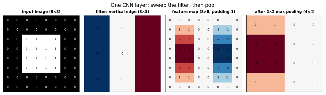
Reading it: left to right, one pass of a CNN layer. The input is an 8×8 image of a bright square on a dark background. The filter is the vertical edge detector from the worked example. The feature map (with padding, so still 8×8) is bright red down the square's left side (dark to bright, the pattern it looks for) and blue down the right side (bright to dark, the opposite pattern); everywhere flat is zero. After 2×2 max pooling the map is 4×4: a quarter of the numbers, but the left edge is still clearly marked. The right edge's negative responses become 0, because max pooling keeps the largest value in each block. Real networks pass maps through ReLU (which zeroes negatives) before pooling anyway, and detect the bright-to-dark edge with a second, mirror-image filter. Numbers in the cells are the actual values.
In code: max_pool2d keeps the largest value in each non-overlapping
block.
A3. Weight sharing and the receptive field
Everyday picture. A rubber stamp: you carve the pattern once and use it everywhere on the page. A CNN uses the same filter at every position, so a cat detector works in any corner of the photo and costs the same number of weights however large the photo is.
Tiny worked example. 64 filters of size 3×3 over a colour image need 3·3·3·64 + 64 = 1,792 parameters, for any image size. A fully connected layer mapping a 224×224×3 image to an output of the same size as those 64 feature maps would need 150,528 × 3,211,264 ≈ 483 billion weights.
As layers stack, each neuron sees more of the original image: its receptive field. One 3×3 layer sees 3×3 pixels; two see 5×5; three see 7×7. Pooling between layers speeds this up: conv 3×3, pool 2×2, conv 3×3 already sees 8×8. That's why two stacked 3×3 filters (18 weights, and two nonlinearities) replaced single 5×5 filters (25 weights) in VGG.
Level 3: the formula and its symbols
$$ r_{\ell} = r_{\ell-1} + (k_\ell - 1)\, j_{\ell-1} \qquad j_\ell = j_{\ell-1}\, s_\ell \qquad r_0 = j_0 = 1 $$
Symbols
| Symbol | Meaning here | Shape / range |
|---|---|---|
| $\ell$ | layer number, counting from the input | 1, 2, 3… |
| $r_\ell$ | receptive field after layer ℓ: input pixels (along one side) one neuron sees | ≥ 1 |
| $k_\ell$ | kernel (filter or pool window) size of layer ℓ | |
| $s_\ell$ | stride of layer ℓ | |
| $j_\ell$ | jump: input pixels between neighbouring neurons at layer ℓ | ≥ 1 |
In words: every layer widens the view by (kernel − 1) steps, and a step at depth ℓ is as many input pixels as all earlier strides multiplied together.
On the worked example: conv 3 (r = 1 + 2·1 = 3, j = 1), pool 2 stride 2 (r = 3 + 1·1 = 4, j = 2), conv 3 (r = 4 + 2·2 = 8).
Level 3: in Python
In Python:
# (k_ℓ, s_ℓ): conv 3, pool 2 with stride 2, conv 3
layers = [(3, 1), (2, 2), (3, 1)]
# r_0 = j_0 = 1
r, j = 1, 1
for k_l, s_l in layers:
    # r_ℓ = r_{ℓ-1} + (k_ℓ - 1) j_{ℓ-1}
    r = r + (k_l - 1) * j
    # j_ℓ = j_{ℓ-1} s_ℓ
    j = j * s_l
    print(r, j)  # → 3 1 4 2 8 2
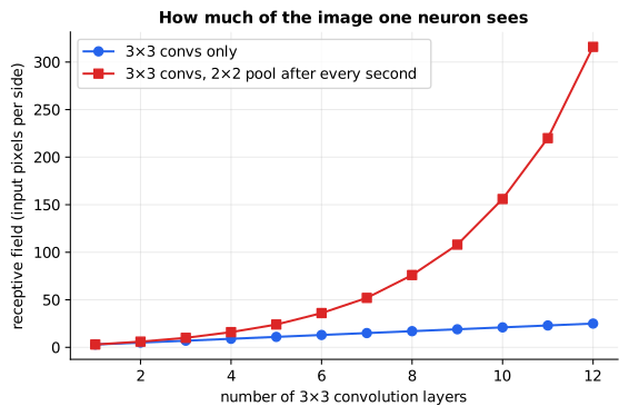
Reading it: the x-axis is the number of 3×3 convolution layers; the y-axis is how many input pixels (along one side) one neuron at that depth can see. Without pooling (lower line) the view grows by 2 pixels per layer, slowly. With a 2×2 pool after every second layer (upper line) the jumps double each time, so a dozen layers already see most of a 224-pixel image. That growth is what lets deep layers recognise whole objects.
In code: conv_params and dense_params count the two layers'
parameters, and receptive_field applies the recurrence to a stack of
(kernel, stride) layers.
A4. From edges to parts to objects
Everyday picture. Reading starts with strokes, then letters, then words, then sentences. A CNN's first layer learns strokes (edges and colour blobs), the next combines them into textures and corners, deeper layers into parts (eyes, wheels), and the last into whole objects.
flowchart LR
  I[Image pixels] --> C1[Conv layer<br/>edges]
  C1 --> P1[Pool]
  P1 --> C2[Conv layer<br/>textures, parts]
  C2 --> P2[Pool]
  P2 --> C3[Conv layer<br/>whole objects]
  C3 --> FC[Dense layer]
  FC --> O[Prediction<br/>cat 94%]
Reading it: each conv layer applies many filters to the feature maps below it, so its patterns are combinations of the patterns below. Each pool halves the resolution, which widens what the next layer sees (section A3). By the end, a small grid of very abstract features feeds an ordinary dense layer that outputs class probabilities. Nobody hand-designs these filters; training discovers them, and first-layer filters in trained networks look remarkably like the edge detectors in this lesson.
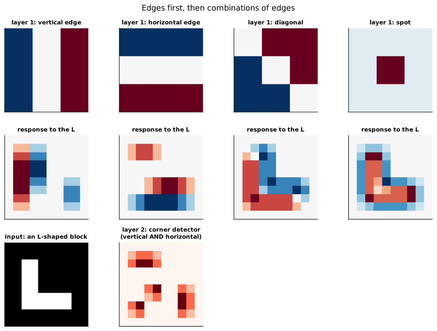
Reading it: the top row shows four 3×3 filters of the kind a first layer learns (red = positive weight, blue = negative): vertical edge, horizontal edge, diagonal, and a centre-surround "spot". The middle row shows each one's response to the same small image of an L-shaped block. The vertical-edge filter fires only on the L's left and right sides (red where dark turns bright, blue where bright turns dark) and the horizontal-edge filter only on its top and bottom. The diagonal filter is not so choosy: its weights lean both ways at once, so it answers about ±2 on every straight side of the L (two thirds of an edge filter's 3) and ±3 at some corners. The spot filter answers faintly (at most about 0.6) all around the outline. One first-layer filter is a weak witness on its own, which is why the next layer combines several. The last panel is a second-layer detector built from first-layer outputs: the vertical-edge strength times the horizontal-edge strength, which is large only where a vertical and a horizontal edge meet, at the L's corners. Combining simple detectors into more specific ones is the whole hierarchy in miniature.
In code: the figure runs each first-layer filter over the L with
conv2d, and the corner detector multiplies two of those feature maps
entry by entry.
A5. Landmarks, and patches as tokens
- AlexNet (2012) won the ImageNet competition by a wide margin by training a deep CNN on GPUs, which started the deep-learning boom.
- VGG (2014) showed that deep stacks of small 3×3 filters work well.
- ResNet (2015) added residual (skip) connections, letting gradients
bypass layers, and made networks of 100+ layers trainable. The same idea
sits inside every transformer (see
primer.ml.deep_nets). - Vision Transformers (2020) cut an image into patches and treat each patch as a token, then apply ordinary attention.
Everyday picture for patches. Cut a photo into a grid of jigsaw pieces, lay them out in a row, and read them like the words of a sentence.
Tiny worked example. A 224×224 colour image cut into 16×16 patches gives (224/16)² = 196 patches, each flattened to 16·16·3 = 768 numbers: 196 tokens of 768 values.
flowchart LR
  IMG[224×224×3 image] --> CUT[Cut into 16×16 patches<br/>14 × 14 = 196 pieces]
  CUT --> FLAT[Flatten each patch<br/>768 numbers]
  FLAT --> PROJ[Linear projection<br/>to model width]
  PROJ --> POS[Add position<br/>embeddings]
  POS --> TF[Transformer blocks<br/>attention across patches]
Reading it: after the cut-and-flatten step, an image is just a sequence of 196 tokens, and everything downstream is the same transformer used for text. Multimodal language models read images mostly this way.
In code: patchify does the cut-and-flatten step, turning an image into
one row of numbers per patch.
Why it matters in practice. CNNs remain efficient and strong for small vision tasks, on-device models and limited data, because their built-in assumptions (locality, weight sharing) mean they learn from less. At large scale, Vision Transformers dominate.
Part B: recurrent networks
B1. An RNN reads with a one-page summary
Everyday picture. You read a book one word at a time, and you are allowed to keep only a single page of notes. After every word you rewrite the page: blend what the page said with the new word. At the end, the page is all you have. That page is the hidden state.
Tiny worked example. The sentence "not very good", with each word turned into one number: not = −1, very = 0.5, good = 1. The summary is a single number h, starting at 0. The rule: new h = tanh(0.5 × old h + 1 × word). (tanh squashes any number into the range −1 to 1: tanh(0) = 0, tanh(1) = 0.76, tanh(−1) = −0.76.)
| step | word | 0.5 × old h + word | new h = tanh(…) |
|---|---|---|---|
| 1 | not (−1) | 0.5 × 0 + (−1) = −1 | −0.762 |
| 2 | very (0.5) | 0.5 × (−0.762) + 0.5 = 0.119 | 0.119 |
| 3 | good (1) | 0.5 × 0.119 + 1 = 1.059 | 0.785 |
The final summary is strongly positive: the "not" at the start has been almost washed out, because the page was rewritten twice since. This is the central weakness of RNNs, in three lines of arithmetic.
flowchart LR
  H0[h0 = 0] --> C1[RNN cell]
  X1[x1: not] --> C1
  C1 --> H1[h1 = −0.762]
  H1 --> C2[RNN cell<br/>same weights]
  X2[x2: very] --> C2
  C2 --> H2[h2 = 0.119]
  H2 --> C3[RNN cell<br/>same weights]
  X3[x3: good] --> C3
  C3 --> H3[h3 = 0.785<br/>final summary]
Reading it: this is one RNN "unrolled in time": the three cells are the same cell with the same weights, drawn once per step. Each step takes the previous summary (arrow from the left) and the next word (arrow from below) and produces the new summary. Everything the network knows about "not" must survive two more rewrites to reach the end.
Level 3: the formula and its symbols
$$ h_t = \tanh\big(W_h\, h_{t-1} + W_x\, x_t + b\big) $$
Symbols
| Symbol | Meaning here | Shape / range |
|---|---|---|
| $t$ | the time step (word position) | 1, 2, 3… |
| $x_t$ | the input at step t (a word's vector) | (inputs,) |
| $h_t$ | the hidden state (the summary page) after step t | (hidden,), each entry in −1…1 |
| $h_{t-1}$ | the summary before this word | (hidden,) |
| $W_h$ | recurrent weights: how the old summary feeds the new one | (hidden, hidden) |
| $W_x$ | input weights: how the word feeds the new summary | (hidden, inputs) |
| $b$ | bias | (hidden,) |
| $\tanh$ | hyperbolic tangent: squashes each number into −1…1 |
In words: the new summary is the squashed sum of the old summary times its weights, the new word times its weights, and a bias.
On the worked example: one-number summary, W_h = 0.5, W_x = 1, b = 0: h₁ = tanh(0.5·0 − 1) = −0.762; h₂ = tanh(0.5·(−0.762) + 0.5) = 0.119; h₃ = tanh(0.5·0.119 + 1) = 0.785.
Level 3: in Python
In Python:
import math
W_h, W_x, b = 0.5, 1, 0
# not, very, good
x = [-1, 0.5, 1]
# h_0: a blank page
h = 0
for x_t in x:
    # h_t = tanh(W_h h_{t-1} + W_x x_t + b)
    h = math.tanh(W_h * h + W_x * x_t + b)
    print(round(h, 3))  # → -0.762 0.119 0.785
In code: RNNCell holds W_h, W_x and b; RNNCell.step is the formula
once, RNNCell.run applies it along a sequence, and RNNCell.scalar builds
the one-number cell of the worked example.
B2. Why RNNs forget: the vanishing gradient
Everyday picture. A photocopy of a photocopy of a photocopy. Each copy loses a little; after twenty copies the original is unreadable. Training an RNN sends a correction signal backwards through every step, and each step multiplies it by a factor. Factors below 1 fade the signal to nothing (vanishing gradient); factors above 1 blow it up (exploding gradient).
Tiny worked example. With a recurrent weight of 0.5 and zero inputs, each step back multiplies the signal by exactly 0.5. Ten steps back: 0.5¹⁰ = 0.00098, about a thousandth. With a weight of 1.5 instead: 1.5¹⁰ = 57.7, and training diverges.
Level 3: the formula and its symbols
$$ \frac{\partial h_T}{\partial h_0} = \prod_{t=1}^{T} \operatorname{diag}!\big(1 - h_t^2\big)\, W_h $$
Symbols
| Symbol | Meaning here | Shape / range |
|---|---|---|
| $\partial h_T / \partial h_0$ | "how much does the final summary change if the starting summary changes a little?" (a derivative, one per pair of entries) | (hidden, hidden) |
| $\prod_{t=1}^{T}$ | multiply the factors for every step from 1 to T | |
| $1 - h_t^2$ | the slope of tanh at step t: 1 near zero, near 0 when tanh saturates | 0…1 |
| $\operatorname{diag}(\cdot)$ | a matrix with these values on the diagonal and zeros elsewhere | (hidden, hidden) |
| $W_h$ | the recurrent weights, as above | (hidden, hidden) |
In words: the influence of the start on the end is the product, over every step, of tanh's slope times the recurrent weights, so it shrinks or grows geometrically with the number of steps.
On the worked example: h stays 0, so every slope is 1, and the product is 0.5 × 0.5 × … (ten times) = 0.00098.
Level 3: in Python
In Python:
W_h = 0.5
# zero inputs keep every h_t at 0
h = [0.0] * 10
influence = 1
for h_t in h:
    # Π over t of tanh's slope times W_h
    influence *= (1 - h_t ** 2) * W_h
round(influence, 5)  # → 0.00098
# the same product with a weight of 1.5
round(1.5 ** 10, 1)  # → 57.7
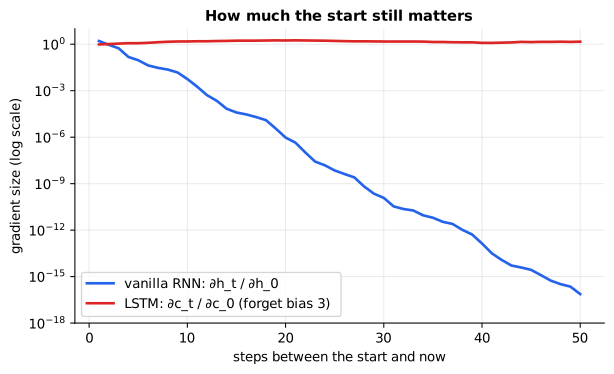
Reading it: the x-axis is how many steps separate the start of the sequence from the current step; the y-axis (log scale) is how strongly the current memory still responds to a nudge in the starting memory. The plain RNN's line plunges: after 20 steps the start has almost no influence, and by 50 it's around 10⁻¹⁶, which means it cannot learn anything about the start. The LSTM's line stays near 1 across all 50 steps. That flat line is the reason LSTMs replaced plain RNNs.
In code: RNNCell.influence_of_start multiplies out the product above
for one sequence, and gradient_through_time measures both lines of the
figure.
B3. LSTM: a notebook with an eraser, a pen and a highlighter
Everyday picture. Instead of rewriting the whole page after every word, keep a notebook (the cell state) and three tools, each controlled by a dial from 0 to 1 that the network sets for itself at every step:
- the eraser (forget gate f): how much of each line to keep;
- the pen (input gate i): how much of the new note to write in;
- the highlighter (output gate o): how much of the notebook to show the outside world right now.
Because the notebook is edited rather than rewritten, information can pass through many steps untouched: eraser off, pen off, and the line survives.
Tiny worked example. One-line notebook holding 0.8.
| eraser keeps f | pen writes i | new note g | highlighter o | new notebook c = f·0.8 + i·g | shown h = o·tanh(c) |
|---|---|---|---|---|---|
| 1 | 0 | – | 1 | 0.8 (kept, even after 100 steps) | 0.664 |
| 0 | 0 | – | 1 | 0 (wiped) | 0 |
| 0 | 1 | 0.5 | 1 | 0.5 (overwritten) | tanh(0.5) = 0.462 |
| 1 | 0 | – | 0 | 0.8 (kept) | 0 (hidden) |
flowchart LR
  CP[notebook c_prev] --> FX((× f<br/>eraser))
  FX --> ADD((+))
  G[new note g] --> IX((× i<br/>pen))
  IX --> ADD
  ADD --> C[notebook c]
  C --> T[tanh]
  T --> OX((× o<br/>highlighter))
  OX --> H[shown h]
  XH[input x and previous h] -.-> FX & IX & OX & G
Reading it: follow the top line: the old notebook is multiplied by the eraser setting, the pen's contribution is added, and the result is the new notebook. There is no squashing on that line, only a multiply and an add, so when the eraser is near 1 the notebook (and the training signal flowing back along it) passes through almost unchanged. The dotted arrows show that all four dials are computed from the current input and the previous shown state, so the network decides at each step what to forget, write and show.
Level 3: the formula and its symbols
$$ \begin{aligned} f_t &= \sigma(W_f [x_t, h_{t-1}] + b_f) &\quad i_t &= \sigma(W_i [x_t, h_{t-1}] + b_i) \ o_t &= \sigma(W_o [x_t, h_{t-1}] + b_o) &\quad g_t &= \tanh(W_g [x_t, h_{t-1}] + b_g) \ c_t &= f_t \odot c_{t-1} + i_t \odot g_t &\quad h_t &= o_t \odot \tanh(c_t) \end{aligned} $$
Symbols
| Symbol | Meaning here | Shape / range |
|---|---|---|
| $f_t, i_t, o_t$ | forget (eraser), input (pen) and output (highlighter) gates | (hidden,), each 0…1 |
| $g_t$ | the candidate note to write | (hidden,), −1…1 |
| $c_t$ | the cell state: the notebook | (hidden,) |
| $h_t$ | the hidden state: what the cell shows | (hidden,) |
| $[x_t, h_{t-1}]$ | the input and previous shown state, stacked into one vector | (inputs + hidden,) |
| $W_f, W_i, W_o, W_g$ | learned weights for each gate | (hidden, inputs + hidden) |
| $\sigma$ | sigmoid, 1/(1 + e⁻ᶻ): squashes to 0…1, so it works as a dial | |
| $\odot$ | multiply element by element (entry 1 with entry 1, and so on) |
In words: three sigmoid dials and one candidate are computed from the input and the previous state; the notebook keeps f of itself and adds i of the candidate; the cell shows o of the squashed notebook.
On the worked example: third row: f = 0, i = 1, g = 0.5, o = 1, so c = 0·0.8 + 1·0.5 = 0.5 and h = 1·tanh(0.5) = 0.462.
Level 3: in Python
In Python:
import math
def sigma(z):
    # σ: any score becomes a dial between 0 and 1
    return 1 / (1 + math.exp(-z))
[round(sigma(z), 3) for z in (-4, 0, 4)]  # → [0.018, 0.5, 0.982]
def lstm_step(f, i, g, o, c_prev=0.8):
    # c_t = f ⊙ c_{t-1} + i ⊙ g
    c = f * c_prev + i * g
    # h_t = o ⊙ tanh(c_t)
    h = o * math.tanh(c)
    return c, h
for f, i, g, o in [(1, 0, 0, 1), (0, 0, 0, 1), (0, 1, 0.5, 1), (1, 0, 0, 0)]:
    # the four rows of the table, dials pinned by hand
    c, h = lstm_step(f, i, g, o)
    print(c, round(h, 3))  # → 0.8 0.664 0.0 0.0 0.5 0.462 0.8 0.0
GRUs simplify this to two dials and no separate notebook: an update gate z chooses between keeping the old state (z = 1) and taking a new candidate (z = 0), and a reset gate decides how much old state feeds that candidate: h = (1 − z) ⊙ n + z ⊙ h_prev, where n is the candidate. Similar performance, fewer parameters.
In code: LSTMCell holds the four gates' stacked weights;
LSTMCell.step computes the dials and updates the notebook,
LSTMCell.run carries it along a sequence, and
LSTMCell.fixed_gates pins the dials to replay the table above;
GRUCell.step is the two-dial version.
B4. Why transformers won
Everyday picture. An RNN is a line of people passing a note: the last person hears about the first only through everyone in between, and nobody can start until the person before them finishes. A transformer is a meeting where everyone can speak to everyone directly, all at once.
Tiny worked example. 1,000 tokens. An RNN needs 1,000 steps one after another, and information from token 1 reaches token 1,000 through 999 hand-offs. A transformer layer processes all 1,000 in 1 parallel step, and any token reaches any other in 1 hop of attention.
flowchart LR
  subgraph RNN["RNN: one step at a time"]
    r1[The] --> r2[cat] --> r3[sat] --> r4[down]
  end
  subgraph TF["Transformer: all at once"]
    t1[The] & t2[cat] & t3[sat] & t4[down] --> A[Attention<br/>every pair compared]
  end
Reading it: in the RNN, information about "The" must survive three
hand-offs to reach "down", and the four steps cannot run at the same time. In
the transformer, all four positions go into attention together and every
pair is compared directly. Parallel training is what made it practical to
train on vastly more data, and that is what led to modern language models.
The price is attention's cost growing with the square of the sequence length
(see primer.ml.attention).
In code: sequential_steps and path_length return the two counts in
the worked example for an RNN or a transformer.
State-space models such as Mamba revisit recurrence with a design that trains in parallel and runs in time linear in sequence length. They carry a compressed state like an RNN but avoid its training bottleneck, and some hybrid models mix them with attention.
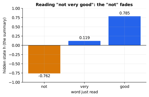
Reading it: the worked example as a picture. Each bar is the one-number summary after reading a word. "not" drives it negative; "very" pulls it back near zero; "good" pushes it strongly positive. The final summary would read as positive sentiment, which is wrong: the negation had to survive two rewrites and didn't. Gates (LSTM) and direct connections (attention) are the two historical fixes.
In 20 seconds
- A convolution slides a small filter across an image, multiplying and adding at each position; the output map shows where the filter's pattern appears.
- Weight sharing (one filter everywhere) and local receptive fields make CNNs efficient; pooling downsamples; depth builds edges → parts → objects.
- An RNN reads one step at a time, carrying a hidden state; backpropagating through many steps multiplies gradients until they vanish or explode.
- LSTMs add a cell state edited by forget, input and output gates, so information and gradients survive many steps.
- Transformers won through parallel training and one-hop paths between any two tokens; Vision Transformers treat image patches as tokens.
Self-test questions
Q: What does one number in a feature map mean? A: How strongly the filter's pattern matches the image patch at that position: the sum of filter weights times the pixels under them.
Q: Why does a CNN need far fewer parameters than a dense layer on images? A: Weight sharing: one small filter is reused at every position, so the parameter count depends on filter size and number of filters, not on image size.
Q: What does pooling buy you? A: Smaller maps (less computation), a faster-growing receptive field, and tolerance to small shifts, since the strongest response in a neighbourhood survives wherever exactly it was.
Q: Why did VGG use stacks of 3×3 filters instead of larger ones? A: Two 3×3 layers see a 5×5 region with 18 weights instead of 25, and add an extra nonlinearity between them.
Q: How does a Vision Transformer turn an image into tokens? A: It cuts the image into fixed-size patches (e.g. 16×16), flattens each into a vector, projects it to the model width and adds a position embedding; the patches are then processed like words.
Q: Why do plain RNNs struggle with long-range dependencies? A: Backpropagation through time multiplies the gradient by the recurrent weights and tanh slopes at every step, so it shrinks geometrically (or explodes) and early inputs stop influencing learning.
Q: How do LSTM gates fix that? A: The cell state is updated additively, c = f ⊙ c_prev + i ⊙ g, so with the forget gate near 1 information and gradients flow through many steps almost unchanged.
Q: Why did transformers replace RNNs? A: RNNs process tokens sequentially, which prevents parallel training, and force all history through one fixed-size state. Attention connects any two tokens in one step and trains all positions in parallel.
Q: What did CNNs contribute that still matters? A: Residual connections (from ResNet), which make very deep networks trainable and are in every transformer block, plus the general lesson that built-in assumptions help when data is limited.
The papers behind this lesson
- He, Zhang, Ren & Sun, Deep Residual Learning for Image Recognition (2015): https://arxiv.org/abs/1512.03385. Introduced residual connections, making networks of 100+ layers trainable. annotated companion
- Vaswani et al., Attention Is All You Need (2017): https://arxiv.org/abs/1706.03762. Replaced recurrence with attention, enabling parallel training and one-hop paths between tokens. annotated companion
- Krizhevsky, Sutskever & Hinton, ImageNet Classification with Deep Convolutional Neural Networks (NeurIPS 2012). Trained a deep CNN on GPUs and won ImageNet by a wide margin, starting the deep-learning boom.
- Simonyan & Zisserman, Very Deep Convolutional Networks for Large-Scale Image Recognition (VGG, 2014): https://arxiv.org/abs/1409.1556. Showed deep stacks of 3×3 filters work well.
- Dosovitskiy et al., An Image is Worth 16x16 Words (ViT, 2020): https://arxiv.org/abs/2010.11929. Applied a plain transformer to image patches as tokens.
- Hochreiter & Schmidhuber, Long Short-Term Memory (1997): https://doi.org/10.1162/neco.1997.9.8.1735. Introduced the gated cell state that carries information across long sequences.
- Cho et al., Learning Phrase Representations using RNN Encoder-Decoder (2014): https://arxiv.org/abs/1406.1078. Introduced the GRU.
- Pascanu, Mikolov & Bengio, On the difficulty of training Recurrent Neural Networks (2012): https://arxiv.org/abs/1211.5063. Analysed vanishing and exploding gradients and proposed gradient clipping.
- Gu & Dao, Mamba: Linear-Time Sequence Modeling with Selective State Spaces (2023): https://arxiv.org/abs/2312.00752. A recurrent-style model that trains in parallel and scales linearly with length.
Further reading
- Stanford CS231n, Convolutional Neural Networks: https://cs231n.github.io/convolutional-networks/
- Christopher Olah, Understanding LSTM Networks: https://colah.github.io/posts/2015-08-Understanding-LSTMs/
- Andrej Karpathy, The Unreasonable Effectiveness of Recurrent Neural Networks: http://karpathy.github.io/2015/05/21/rnn-effectiveness/
- Olah, Mordvintsev & Schubert, Feature Visualization (Distill): https://distill.pub/2017/feature-visualization/
1r""" 2# CNNs and RNNs: how networks see images and read sequences 3 4Run: `python -m primer.ml.cnn_rnn` 5 6New to the notation? `primer.notation` explains every symbol used here 7(Σ, ⊙, subscripts, ∂, and so on) from zero. This lesson builds on 8`primer.ml.neural_net` and `primer.ml.attention`. 9 10## Level 1: The practitioner's guide 11 12**In one sentence.** Convolutional networks see images by sliding small 13learned pattern detectors across them, recurrent networks read sequences one 14step at a time with a running memory, and knowing what each does well and 15where each breaks tells you when to reach for one, when to reach for a 16transformer instead, and why images cost what they cost in a multimodal 17model. 18 19**When you need it.** Not for a chat product on a hosted model: there the 20transformer has already won and this lesson is background. You need it when 21you have an image or signal problem of your own to solve: a defect detector 22for a production line, a model that must run on a phone or a camera, a time 23series or sensor stream, a legacy system built on LSTMs that you now 24maintain, or a bill for image inputs that you want to predict. The tell: a 25dataset that is not text, or a device that is not a GPU. The number behind 26the first choice, from this lesson's `conv_params` and `dense_params`: 64 27filters of 3 × 3 over a colour image need 1,792 parameters, at any image 28size, while a dense layer mapping a 224 × 224 colour image to an output of 29the same size needs about 483 billion. Built-in assumptions (patterns are 30local, the same pattern matters anywhere) are what make vision affordable 31from little data. 32 33**Your options.** Two families for images, three for sequences, and the 34transformer that now spans both. From the most specialised to the most 35general: 36 37| Option | What it does | What it gives you | What it costs | Where it lives | 38|---|---|---|---|---| 39| A convolutional network (ResNet family) | Slides learned filters over the image, pools, stacks edges into parts into objects | Strong results from modest data and modest hardware; 1,792 parameters for 64 filters | Its locality assumption caps it at the largest scales | Vision libraries and on-device runtimes | 40| A vision transformer (ViT) | Cuts the image into patches, treats each as a token, runs ordinary attention | The best accuracy at scale, on the same stack as text; its paper reports better results than the leading CNNs with substantially less training compute | Needs large pretraining data; 196 tokens for a 224 × 224 image at 16-pixel patches | Vision backbones and multimodal models | 41| An image sent to a multimodal LLM | Patches become tokens beside your text | No model to train; you ask questions about the picture | Billed per patch: Claude counts one visual token per 28 × 28 block, so a 1000 × 1000 image is 1,296 tokens | Hosted APIs | 42| A plain recurrent network | Rewrites one summary vector after every step | The smallest possible state; runs on anything | Forgets: the start's influence is 0.5¹⁰, about a thousandth, ten steps back in this lesson's example | Legacy and tiny embedded models | 43| An LSTM or GRU | Keeps a gated cell state that is edited, not rewritten | Memory across hundreds of steps: the gradient stays near 1 after 50 steps where the plain RNN's is around 10⁻¹⁶ | Sequential training, one step per token; superseded for language | Legacy NLP, time series, small sequence models | 44| A transformer | Compares every token with every other in one parallel step | Parallel training and a one-hop path between any two tokens | Cost that grows with the square of the length (`primer.ml.attention`) | Every modern language model | 45| A state-space model (Mamba) | A selective recurrence that trains in parallel and runs in linear time | 5× the inference throughput of a transformer in its paper, with a fixed-size state | Fewer mature models; some hybrids mix it with attention | Long-stream and hybrid models | 46 47**How to choose.** Start from the data, then the device. 48 49- Images, limited data or a small device: a convolutional network, 50 pretrained if you can get one. Weight sharing and locality mean it learns 51 from less and runs in a fixed budget of parameters. 52- Images at scale, or images beside text: a vision transformer or a 53 multimodal model. Count the tokens an image will cost before you build 54 the pipeline. 55- Sequences of any kind today: a transformer by default. Keep an LSTM or 56 GRU only for tiny streaming models, or where a legacy system already 57 works. 58- Very long streams where throughput matters more than exact recall: a 59 state-space model or a hybrid, measured against a transformer on your 60 data. 61- Anything deep, of any family: residual connections. A 34-layer plain 62 network scored worse than an 18-layer one on ImageNet (28.54% against 63 27.94% top-1 error) until shortcuts took it to 25.03%. 64- Whatever you pick, benchmark at your own scale: the crossover between 65 built-in assumptions and raw data is different for every dataset. 66 67**What it costs.** Parameters, compute, and the sequential steps that 68nobody can parallelize. 69 70- Parameters. A convolution's cost depends on the filter and the channel 71 counts, never on the image size: 1,792 for the 64 filters above. A dense 72 layer on raw pixels is out of the question at 483 billion. 73- Compute. ResNet-152 runs in 11.3 billion operations per image against 74 VGG-16's 15.3 billion, deeper and cheaper at once (the ResNet companion). 75 A 224 × 224 image is 196 tokens of 768 numbers to a vision transformer 76 (`patchify`), and attention over those tokens is the same n² as for text. 77- Sequential steps. An RNN reading 1,000 tokens takes 1,000 steps one after 78 another, and information from the first token reaches the last through 79 999 hand-offs; a transformer layer does it in one step and one hop 80 (`sequential_steps`, `path_length`). That difference is why transformers 81 could train on vastly more data. 82- Memory. An RNN's state is one vector however long the input; a 83 transformer keeps keys and values for every token (`primer.ml.inference`). 84 That is the trade state-space models revisit. 85 86**What breaks.** 87 88- **A summary that forgets the start.** Reading "not very good" one word at 89 a time, this lesson's one-number RNN ends at 0.785, strongly positive, 90 because "not" was rewritten away two steps later. Gates or attention are 91 the fixes. 92- **Gradients that vanish or explode.** Each step back multiplies the 93 training signal by a factor: 0.5 gives 0.00098 after ten steps, 1.5 gives 94 57.7 and diverges. Clip gradients (Pascanu et al., 2012) and use gated 95 cells. 96- **Depth that makes things worse.** Without shortcuts a deeper network can 97 score lower even on its training data; residual connections reverse it 98 and are inside every transformer block. 99- **A view too narrow for the object.** One 3 × 3 layer sees 3 pixels; 100 conv, pool, conv sees 8 (`receptive_field`). A shallow network without 101 pooling never sees a whole object, however many filters it has. 102- **Image bills that scale with pixels.** Every patch is a token: on 103 Anthropic's API an image costs ⌈width / 28⌉ × ⌈height / 28⌉ visual tokens, 104 so a 200 × 200 image is 64 tokens and a 1000 × 1000 image is 1,296, about 105 \$1.30 per thousand images at \$1 per million tokens. Resize before you 106 send. 107- **Patches with no positions.** A vision transformer reads a bag of 108 patches unless positions are added, exactly as text does 109 (`primer.ml.positional`). 110 111**In the wild.** AlexNet won ImageNet in 2012 by training a deep CNN on 112GPUs; VGG showed that stacks of 3 × 3 filters work; ResNet's 152-layer 113network reached 3.57% top-5 error in an ensemble and put the shortcut 114connection into every architecture since. Vision transformers took over 115large-scale vision, and multimodal language models read images the same 116way, as patch tokens. On the sequence side, the LSTM (Hochreiter and 117Schmidhuber, 1997) and the GRU (Cho et al., 2014) carried language modelling 118until attention, and Mamba (Gu and Dao, 2023) reports a 3-billion-parameter 119model matching transformers twice its size at linear cost in length. The 120papers are linked at the end of the lesson. 121 122**Go deeper.** Level 2 runs a 3 × 3 edge filter over a 5 × 5 image by hand, 123pools a 4 × 4 map, counts receptive fields, cuts an image into patch tokens, 124reads "not very good" with a one-number RNN, multiplies out the vanishing 125gradient, pins an LSTM's gates to keep, erase, overwrite and hide a note, 126and counts the steps that decided the contest. If you only needed to choose 127a family, you are done. 128 129## Level 2: How it works, from scratch 130 131Before transformers, two designs dominated deep learning, and both still 132matter. **Convolutional networks (CNNs)** see images by sliding small 133pattern detectors across them. **Recurrent networks (RNNs)** read sequences 134one item at a time, carrying a running memory. Each builds in an assumption 135about its data (patterns in images are local; sequences unfold in order), 136and each has a limit that the transformer removed. Knowing both stories 137explains why modern models look the way they do. 138 139# Part A: convolutional networks 140 141## A1. A convolution is a flashlight looking for one pattern 142 143**Everyday picture.** You are in a dark room with a large photograph and a 144small flashlight. You're looking for one thing, say a place where dark turns 145to bright from left to right. You sweep the flashlight across the photo, one 146step at a time, and at every spot you jot down a score: high if the lit 147patch matches what you're looking for, near zero if it doesn't. When you 148finish, your notes form a new, smaller picture: a map of *where* the pattern 149appears. That map is called a **feature map**, and the pattern you were 150looking for, written as a small grid of numbers, is the **filter** (or 151kernel). 152 153**Tiny worked example.** A 5×5 image: two dark columns (0) then three bright 154columns (1), so there is a vertical edge between columns 2 and 3. The filter 155is a 3×3 "vertical edge" detector: −1 on the left column, 0 in the middle, 156+1 on the right. It rewards "bright on the right, dark on the left". 157 158``` 159image X filter K 1600 0 1 1 1 -1 0 1 1610 0 1 1 1 -1 0 1 1620 0 1 1 1 -1 0 1 1630 0 1 1 1 1640 0 1 1 1 165``` 166 167Put the filter on the top-left 3×3 patch of the image. Multiply each image 168number by the filter number on top of it, and add all nine products: 169 170``` 171patch × filter = products 1720 0 1 -1 0 1 0 0 1 1730 0 1 -1 0 1 0 0 1 sum = 1 + 1 + 1 = 3 1740 0 1 -1 0 1 0 0 1 175``` 176 177So the top-left cell of the feature map is **3**. Slide one step right: the 178patch is `0 1 1` in every row; products `0 0 1` per row; sum again **3** 179(the edge is still under the flashlight). One more step: the patch is 180`1 1 1`, products `−1 0 1`, sum **0** (flat bright area, no edge). Doing the 181same for every row gives the full 3×3 feature map: 182 183``` 1843 3 0 1853 3 0 1863 3 0 187``` 188 189The high numbers sit exactly where the edge is. Run a *horizontal* edge 190filter over the same image and every cell is 0: this image has no 191top-to-bottom change. Each filter answers one question. 192 193```mermaid 194flowchart LR 195 W[Take the next k×k patch<br/>of the image] --> M[Multiply each pixel by the<br/>filter weight on top of it] 196 M --> S[Add all the products<br/>into one number] 197 S --> C[Write it into the<br/>feature map] 198 C --> N{More positions?} 199 N -->|slide by the stride| W 200 N -->|no| F[Feature map complete] 201``` 202 203**Reading it:** this loop *is* a convolution. The only arithmetic is 204multiply-and-add, repeated at every position. The stride is how far the 205flashlight jumps each time (1 pixel, or 2 to shrink the output faster). 206Padding adds a border of zeros so the filter can also centre on edge pixels 207and the output keeps the input's size. 208 209$$ 210Y[i, j] = \sum_{c}\sum_{u=0}^{k-1}\sum_{v=0}^{k-1} K[c, u, v]\; X[c,\; i\,s + u,\; j\,s + v] 211\qquad 212\text{out} = \left\lfloor \frac{n + 2p - k}{s} \right\rfloor + 1 213$$ 214 215**Symbols** 216 217| Symbol | Meaning here | Shape / range | 218|---|---|---| 219| $X$ | the input image; $X[c, a, b]$ is channel c (red, green or blue) at row a, column b | (channels, height, width) | 220| $K$ | the filter (kernel): a small grid of learned weights, one slice per channel | (channels, k, k) | 221| $Y[i, j]$ | the feature-map value at output row i, column j | one number | 222| $\sum_c \sum_u \sum_v$ | add up over every channel c and every filter row u and column v | | 223| $k$ | filter size (3 for a 3×3 filter) | small integer | 224| $s$ | stride: how many pixels the filter jumps between positions | 1 or 2 | 225| $n$ | input size along one side | e.g. 5 or 224 | 226| $p$ | padding: zeros added around each side | 0, 1, 2… | 227| $\lfloor \cdot \rfloor$ | floor: round down to a whole number | | 228 229**In words:** each output number is the sum, over the filter's footprint and 230all colour channels, of filter weight times the pixel under it; the output 231has one number per place the filter can stand. 232 233**On the worked example:** one channel, k = 3, s = 1, p = 0. Y[0, 0] = 234(−1)·0 + 0·0 + 1·1 for each of the 3 rows = 3. Output size 235⌊(5 + 0 − 3)/1⌋ + 1 = 3. For a 224-pixel image, a 7×7 filter, stride 2 and 236padding 3: ⌊(224 + 6 − 7)/2⌋ + 1 = 112. 237 238**In Python:** 239 240```python 241# the 5×5 image: one channel, so Σ_c has one term 242X = [[0, 0, 1, 1, 1] for _ in range(5)] 243# the vertical-edge filter 244K = [[-1, 0, 1] for _ in range(3)] 245n, k, s, p = 5, 3, 1, 0 246# ⌊(n + 2p - k) / s⌋ + 1 247out = (n + 2 * p - k) // s + 1 248out # → 3 249# Σ_u Σ_v K[u, v] X[i s + u, j s + v] 250Y = [[sum(K[u][v] * X[i * s + u][j * s + v] 251 for u in range(k) for v in range(k)) 252 for j in range(out)] 253 for i in range(out)] 254Y # → [[3, 3, 0], [3, 3, 0], [3, 3, 0]] 255# 224 pixels, 7×7 filter, stride 2, padding 3 256(224 + 2 * 3 - 7) // 2 + 1 # → 112 257``` 258 259**In code:** `conv2d` is the loop in the diagram, one multiply-and-add per 260position, and `conv_output_size` is the output-size formula. 261 262## A2. Pooling: summarise each neighbourhood by its loudest voice 263 264**Everyday picture.** A manager asks each of four teams for one number: the 265strongest signal anyone on the team saw. The report is four times shorter 266and still says where something important happened. 267 268**Tiny worked example.** 2×2 max pooling on a 4×4 map keeps the largest 269value in each quarter: 270 271``` 2721 3 | 0 0 2732 4 | 0 1 -> 4 1 274----+---- 1 6 2750 0 | 5 2 2761 0 | 1 6 277``` 278 279 280 281**Reading it:** left to right, one pass of a CNN layer. The input is an 8×8 282image of a bright square on a dark background. The filter is the vertical 283edge detector from the worked example. The feature map (with padding, so 284still 8×8) is bright red down the square's left side (dark to bright, the 285pattern it looks for) and blue down the right side (bright to dark, the 286opposite pattern); everywhere flat is zero. After 2×2 max pooling the map 287is 4×4: a quarter of the numbers, but the left edge is still clearly marked. 288The right edge's negative responses become 0, because max pooling keeps the 289*largest* value in each block. Real networks pass maps through ReLU (which 290zeroes negatives) before pooling anyway, and detect the bright-to-dark edge 291with a second, mirror-image filter. Numbers in the cells are the actual 292values. 293 294**In code:** `max_pool2d` keeps the largest value in each non-overlapping 295block. 296 297## A3. Weight sharing and the receptive field 298 299**Everyday picture.** A rubber stamp: you carve the pattern once and use it 300everywhere on the page. A CNN uses the *same* filter at every position, 301so a cat detector works in any corner of the photo and costs the same 302number of weights however large the photo is. 303 304**Tiny worked example.** 64 filters of size 3×3 over a colour image need 3053·3·3·64 + 64 = **1,792** parameters, for any image size. A fully connected 306layer mapping a 224×224×3 image to an output of the same size as those 64 307feature maps would need 150,528 × 3,211,264 ≈ **483 billion** weights. 308 309As layers stack, each neuron sees more of the original image: its 310**receptive field**. One 3×3 layer sees 3×3 pixels; two see 5×5; three see 3117×7. Pooling between layers speeds this up: conv 3×3, pool 2×2, conv 3×3 312already sees 8×8. That's why two stacked 3×3 filters (18 weights, and two 313nonlinearities) replaced single 5×5 filters (25 weights) in VGG. 314 315$$ 316r_{\ell} = r_{\ell-1} + (k_\ell - 1)\, j_{\ell-1} \qquad j_\ell = j_{\ell-1}\, s_\ell \qquad r_0 = j_0 = 1 317$$ 318 319**Symbols** 320 321| Symbol | Meaning here | Shape / range | 322|---|---|---| 323| $\ell$ | layer number, counting from the input | 1, 2, 3… | 324| $r_\ell$ | receptive field after layer ℓ: input pixels (along one side) one neuron sees | ≥ 1 | 325| $k_\ell$ | kernel (filter or pool window) size of layer ℓ | | 326| $s_\ell$ | stride of layer ℓ | | 327| $j_\ell$ | jump: input pixels between neighbouring neurons at layer ℓ | ≥ 1 | 328 329**In words:** every layer widens the view by (kernel − 1) steps, and a step 330at depth ℓ is as many input pixels as all earlier strides multiplied 331together. 332 333**On the worked example:** conv 3 (r = 1 + 2·1 = 3, j = 1), pool 2 stride 2 334(r = 3 + 1·1 = 4, j = 2), conv 3 (r = 4 + 2·2 = 8). 335 336**In Python:** 337 338```python 339# (k_ℓ, s_ℓ): conv 3, pool 2 with stride 2, conv 3 340layers = [(3, 1), (2, 2), (3, 1)] 341# r_0 = j_0 = 1 342r, j = 1, 1 343for k_l, s_l in layers: 344 # r_ℓ = r_{ℓ-1} + (k_ℓ - 1) j_{ℓ-1} 345 r = r + (k_l - 1) * j 346 # j_ℓ = j_{ℓ-1} s_ℓ 347 j = j * s_l 348 print(r, j) # → 3 1 4 2 8 2 349``` 350 351 352 353**Reading it:** the x-axis is the number of 3×3 convolution layers; the 354y-axis is how many input pixels (along one side) one neuron at that depth 355can see. Without pooling (lower line) the view grows by 2 pixels per layer, 356slowly. With a 2×2 pool after every second layer (upper line) the jumps 357double each time, so a dozen layers already see most of a 224-pixel image. 358That growth is what lets deep layers recognise whole objects. 359 360**In code:** `conv_params` and `dense_params` count the two layers' 361parameters, and `receptive_field` applies the recurrence to a stack of 362(kernel, stride) layers. 363 364## A4. From edges to parts to objects 365 366**Everyday picture.** Reading starts with strokes, then letters, then words, 367then sentences. A CNN's first layer learns strokes (edges and colour 368blobs), the next combines them into textures and corners, deeper layers 369into parts (eyes, wheels), and the last into whole objects. 370 371```mermaid 372flowchart LR 373 I[Image pixels] --> C1[Conv layer<br/>edges] 374 C1 --> P1[Pool] 375 P1 --> C2[Conv layer<br/>textures, parts] 376 C2 --> P2[Pool] 377 P2 --> C3[Conv layer<br/>whole objects] 378 C3 --> FC[Dense layer] 379 FC --> O[Prediction<br/>cat 94%] 380``` 381 382**Reading it:** each conv layer applies many filters to the feature maps 383below it, so its patterns are combinations of the patterns below. Each pool 384halves the resolution, which widens what the next layer sees (section A3). 385By the end, a small grid of very abstract features feeds an ordinary dense 386layer that outputs class probabilities. Nobody hand-designs these filters; 387training discovers them, and first-layer filters in trained networks look 388remarkably like the edge detectors in this lesson. 389 390 391 392**Reading it:** the top row shows four 3×3 filters of the kind a first 393layer learns (red = positive weight, blue = negative): vertical edge, 394horizontal edge, diagonal, and a centre-surround "spot". The middle row 395shows each one's response to the same small image of an L-shaped block. 396The vertical-edge filter fires only on the L's left and right sides (red 397where dark turns bright, blue where bright turns dark) and the 398horizontal-edge filter only on its top and bottom. The diagonal filter is 399not so choosy: its weights lean both ways at once, so it answers about ±2 on 400*every* straight side of the L (two thirds of an edge filter's 3) and ±3 at 401some corners. The spot filter answers faintly (at most about 0.6) all around 402the outline. One first-layer filter is a weak witness on its own, which is 403why the next layer combines several. The last panel is a second-layer 404detector built from first-layer outputs: the vertical-edge strength times 405the horizontal-edge strength, which is large only where a vertical *and* a 406horizontal edge meet, at the L's corners. Combining simple detectors into 407more specific ones is the whole hierarchy in miniature. 408 409**In code:** the figure runs each first-layer filter over the L with 410`conv2d`, and the corner detector multiplies two of those feature maps 411entry by entry. 412 413## A5. Landmarks, and patches as tokens 414 415- **AlexNet (2012)** won the ImageNet competition by a wide margin by training 416 a deep CNN on GPUs, which started the deep-learning boom. 417- **VGG (2014)** showed that deep stacks of small 3×3 filters work well. 418- **ResNet (2015)** added residual (skip) connections, letting gradients 419 bypass layers, and made networks of 100+ layers trainable. The same idea 420 sits inside every transformer (see `primer.ml.deep_nets`). 421- **Vision Transformers (2020)** cut an image into patches and treat each 422 patch as a token, then apply ordinary attention. 423 424**Everyday picture for patches.** Cut a photo into a grid of jigsaw pieces, 425lay them out in a row, and read them like the words of a sentence. 426 427**Tiny worked example.** A 224×224 colour image cut into 16×16 patches gives 428(224/16)² = **196** patches, each flattened to 16·16·3 = **768** numbers: 429196 tokens of 768 values. 430 431```mermaid 432flowchart LR 433 IMG[224×224×3 image] --> CUT[Cut into 16×16 patches<br/>14 × 14 = 196 pieces] 434 CUT --> FLAT[Flatten each patch<br/>768 numbers] 435 FLAT --> PROJ[Linear projection<br/>to model width] 436 PROJ --> POS[Add position<br/>embeddings] 437 POS --> TF[Transformer blocks<br/>attention across patches] 438``` 439 440**Reading it:** after the cut-and-flatten step, an image is just a sequence 441of 196 tokens, and everything downstream is the same transformer used for 442text. Multimodal language models read images mostly this way. 443 444**In code:** `patchify` does the cut-and-flatten step, turning an image into 445one row of numbers per patch. 446 447**Why it matters in practice.** CNNs remain efficient and strong for small 448vision tasks, on-device models and limited data, because their built-in 449assumptions (locality, weight sharing) mean they learn from less. At large 450scale, Vision Transformers dominate. 451 452# Part B: recurrent networks 453 454## B1. An RNN reads with a one-page summary 455 456**Everyday picture.** You read a book one word at a time, and you are 457allowed to keep only a single page of notes. After every word you rewrite 458the page: blend what the page said with the new word. At the end, the page 459is all you have. That page is the **hidden state**. 460 461**Tiny worked example.** The sentence "not very good", with each word turned 462into one number: not = −1, very = 0.5, good = 1. The summary is a single 463number h, starting at 0. The rule: new h = tanh(0.5 × old h + 1 × word). 464(tanh squashes any number into the range −1 to 1: tanh(0) = 0, 465tanh(1) = 0.76, tanh(−1) = −0.76.) 466 467| step | word | 0.5 × old h + word | new h = tanh(…) | 468|---|---|---|---| 469| 1 | not (−1) | 0.5 × 0 + (−1) = −1 | **−0.762** | 470| 2 | very (0.5) | 0.5 × (−0.762) + 0.5 = 0.119 | **0.119** | 471| 3 | good (1) | 0.5 × 0.119 + 1 = 1.059 | **0.785** | 472 473The final summary is strongly positive: the "not" at the start has been 474almost washed out, because the page was rewritten twice since. This is the 475central weakness of RNNs, in three lines of arithmetic. 476 477```mermaid 478flowchart LR 479 H0[h0 = 0] --> C1[RNN cell] 480 X1[x1: not] --> C1 481 C1 --> H1[h1 = −0.762] 482 H1 --> C2[RNN cell<br/>same weights] 483 X2[x2: very] --> C2 484 C2 --> H2[h2 = 0.119] 485 H2 --> C3[RNN cell<br/>same weights] 486 X3[x3: good] --> C3 487 C3 --> H3[h3 = 0.785<br/>final summary] 488``` 489 490**Reading it:** this is one RNN "unrolled in time": the three cells are the 491*same* cell with the *same* weights, drawn once per step. Each step takes the 492previous summary (arrow from the left) and the next word (arrow from below) 493and produces the new summary. Everything the network knows about "not" must 494survive two more rewrites to reach the end. 495 496$$ 497h_t = \tanh\big(W_h\, h_{t-1} + W_x\, x_t + b\big) 498$$ 499 500**Symbols** 501 502| Symbol | Meaning here | Shape / range | 503|---|---|---| 504| $t$ | the time step (word position) | 1, 2, 3… | 505| $x_t$ | the input at step t (a word's vector) | (inputs,) | 506| $h_t$ | the hidden state (the summary page) after step t | (hidden,), each entry in −1…1 | 507| $h_{t-1}$ | the summary before this word | (hidden,) | 508| $W_h$ | recurrent weights: how the old summary feeds the new one | (hidden, hidden) | 509| $W_x$ | input weights: how the word feeds the new summary | (hidden, inputs) | 510| $b$ | bias | (hidden,) | 511| $\tanh$ | hyperbolic tangent: squashes each number into −1…1 | | 512 513**In words:** the new summary is the squashed sum of the old summary times 514its weights, the new word times its weights, and a bias. 515 516**On the worked example:** one-number summary, W_h = 0.5, W_x = 1, b = 0: 517h₁ = tanh(0.5·0 − 1) = −0.762; h₂ = tanh(0.5·(−0.762) + 0.5) = 0.119; 518h₃ = tanh(0.5·0.119 + 1) = 0.785. 519 520**In Python:** 521 522```python 523import math 524W_h, W_x, b = 0.5, 1, 0 525# not, very, good 526x = [-1, 0.5, 1] 527# h_0: a blank page 528h = 0 529for x_t in x: 530 # h_t = tanh(W_h h_{t-1} + W_x x_t + b) 531 h = math.tanh(W_h * h + W_x * x_t + b) 532 print(round(h, 3)) # → -0.762 0.119 0.785 533``` 534 535**In code:** `RNNCell` holds W_h, W_x and b; `RNNCell.step` is the formula 536once, `RNNCell.run` applies it along a sequence, and `RNNCell.scalar` builds 537the one-number cell of the worked example. 538 539## B2. Why RNNs forget: the vanishing gradient 540 541**Everyday picture.** A photocopy of a photocopy of a photocopy. Each copy 542loses a little; after twenty copies the original is unreadable. Training an 543RNN sends a correction signal *backwards* through every step, and each step 544multiplies it by a factor. Factors below 1 fade the signal to nothing 545(**vanishing gradient**); factors above 1 blow it up (**exploding 546gradient**). 547 548**Tiny worked example.** With a recurrent weight of 0.5 and zero inputs, each 549step back multiplies the signal by exactly 0.5. Ten steps back: 0.5¹⁰ = 550**0.00098**, about a thousandth. With a weight of 1.5 instead: 1.5¹⁰ = 551**57.7**, and training diverges. 552 553$$ 554\frac{\partial h_T}{\partial h_0} = \prod_{t=1}^{T} \operatorname{diag}\!\big(1 - h_t^2\big)\, W_h 555$$ 556 557**Symbols** 558 559| Symbol | Meaning here | Shape / range | 560|---|---|---| 561| $\partial h_T / \partial h_0$ | "how much does the final summary change if the starting summary changes a little?" (a derivative, one per pair of entries) | (hidden, hidden) | 562| $\prod_{t=1}^{T}$ | multiply the factors for every step from 1 to T | | 563| $1 - h_t^2$ | the slope of tanh at step t: 1 near zero, near 0 when tanh saturates | 0…1 | 564| $\operatorname{diag}(\cdot)$ | a matrix with these values on the diagonal and zeros elsewhere | (hidden, hidden) | 565| $W_h$ | the recurrent weights, as above | (hidden, hidden) | 566 567**In words:** the influence of the start on the end is the product, over 568every step, of tanh's slope times the recurrent weights, so it shrinks or 569grows geometrically with the number of steps. 570 571**On the worked example:** h stays 0, so every slope is 1, and the product 572is 0.5 × 0.5 × … (ten times) = 0.00098. 573 574**In Python:** 575 576```python 577W_h = 0.5 578# zero inputs keep every h_t at 0 579h = [0.0] * 10 580influence = 1 581for h_t in h: 582 # Π over t of tanh's slope times W_h 583 influence *= (1 - h_t ** 2) * W_h 584round(influence, 5) # → 0.00098 585# the same product with a weight of 1.5 586round(1.5 ** 10, 1) # → 57.7 587``` 588 589 590 591**Reading it:** the x-axis is how many steps separate the start of the 592sequence from the current step; the y-axis (log scale) is how strongly the 593current memory still responds to a nudge in the starting memory. The plain 594RNN's line plunges: after 20 steps the start has almost no influence, and by 59550 it's around 10⁻¹⁶, which means it cannot learn anything about the start. 596The LSTM's line stays near 1 across all 50 steps. That flat line is the 597reason LSTMs replaced plain RNNs. 598 599**In code:** `RNNCell.influence_of_start` multiplies out the product above 600for one sequence, and `gradient_through_time` measures both lines of the 601figure. 602 603## B3. LSTM: a notebook with an eraser, a pen and a highlighter 604 605**Everyday picture.** Instead of rewriting the whole page after every word, 606keep a notebook (the **cell state**) and three tools, each controlled by a 607dial from 0 to 1 that the network sets for itself at every step: 608 609- the **eraser** (forget gate f): how much of each line to keep; 610- the **pen** (input gate i): how much of the new note to write in; 611- the **highlighter** (output gate o): how much of the notebook to show the 612 outside world right now. 613 614Because the notebook is *edited* rather than rewritten, information can pass 615through many steps untouched: eraser off, pen off, and the line survives. 616 617**Tiny worked example.** One-line notebook holding 0.8. 618 619| eraser keeps f | pen writes i | new note g | highlighter o | new notebook c = f·0.8 + i·g | shown h = o·tanh(c) | 620|---|---|---|---|---|---| 621| 1 | 0 | – | 1 | 0.8 (kept, even after 100 steps) | 0.664 | 622| 0 | 0 | – | 1 | 0 (wiped) | 0 | 623| 0 | 1 | 0.5 | 1 | 0.5 (overwritten) | tanh(0.5) = 0.462 | 624| 1 | 0 | – | 0 | 0.8 (kept) | 0 (hidden) | 625 626```mermaid 627flowchart LR 628 CP[notebook c_prev] --> FX((× f<br/>eraser)) 629 FX --> ADD((+)) 630 G[new note g] --> IX((× i<br/>pen)) 631 IX --> ADD 632 ADD --> C[notebook c] 633 C --> T[tanh] 634 T --> OX((× o<br/>highlighter)) 635 OX --> H[shown h] 636 XH[input x and previous h] -.-> FX & IX & OX & G 637``` 638 639**Reading it:** follow the top line: the old notebook is multiplied by the 640eraser setting, the pen's contribution is *added*, and the result is the new 641notebook. There is no squashing on that line, only a multiply and an add, 642so when the eraser is near 1 the notebook (and the training signal flowing 643back along it) passes through almost unchanged. The dotted arrows show that 644all four dials are computed from the current input and the previous shown 645state, so the network decides at each step what to forget, write and show. 646 647$$ 648\begin{aligned} 649f_t &= \sigma(W_f [x_t, h_{t-1}] + b_f) &\quad i_t &= \sigma(W_i [x_t, h_{t-1}] + b_i) \\ 650o_t &= \sigma(W_o [x_t, h_{t-1}] + b_o) &\quad g_t &= \tanh(W_g [x_t, h_{t-1}] + b_g) \\ 651c_t &= f_t \odot c_{t-1} + i_t \odot g_t &\quad h_t &= o_t \odot \tanh(c_t) 652\end{aligned} 653$$ 654 655**Symbols** 656 657| Symbol | Meaning here | Shape / range | 658|---|---|---| 659| $f_t, i_t, o_t$ | forget (eraser), input (pen) and output (highlighter) gates | (hidden,), each 0…1 | 660| $g_t$ | the candidate note to write | (hidden,), −1…1 | 661| $c_t$ | the cell state: the notebook | (hidden,) | 662| $h_t$ | the hidden state: what the cell shows | (hidden,) | 663| $[x_t, h_{t-1}]$ | the input and previous shown state, stacked into one vector | (inputs + hidden,) | 664| $W_f, W_i, W_o, W_g$ | learned weights for each gate | (hidden, inputs + hidden) | 665| $\sigma$ | sigmoid, 1/(1 + e⁻ᶻ): squashes to 0…1, so it works as a dial | | 666| $\odot$ | multiply element by element (entry 1 with entry 1, and so on) | | 667 668**In words:** three sigmoid dials and one candidate are computed from the 669input and the previous state; the notebook keeps f of itself and adds i of 670the candidate; the cell shows o of the squashed notebook. 671 672**On the worked example:** third row: f = 0, i = 1, g = 0.5, o = 1, so 673c = 0·0.8 + 1·0.5 = 0.5 and h = 1·tanh(0.5) = 0.462. 674 675**In Python:** 676 677```python 678import math 679def sigma(z): 680 # σ: any score becomes a dial between 0 and 1 681 return 1 / (1 + math.exp(-z)) 682[round(sigma(z), 3) for z in (-4, 0, 4)] # → [0.018, 0.5, 0.982] 683def lstm_step(f, i, g, o, c_prev=0.8): 684 # c_t = f ⊙ c_{t-1} + i ⊙ g 685 c = f * c_prev + i * g 686 # h_t = o ⊙ tanh(c_t) 687 h = o * math.tanh(c) 688 return c, h 689for f, i, g, o in [(1, 0, 0, 1), (0, 0, 0, 1), (0, 1, 0.5, 1), (1, 0, 0, 0)]: 690 # the four rows of the table, dials pinned by hand 691 c, h = lstm_step(f, i, g, o) 692 print(c, round(h, 3)) # → 0.8 0.664 0.0 0.0 0.5 0.462 0.8 0.0 693``` 694 695**GRUs** simplify this to two dials and no separate notebook: an *update* 696gate z chooses between keeping the old state (z = 1) and taking a new 697candidate (z = 0), and a *reset* gate decides how much old state feeds that 698candidate: h = (1 − z) ⊙ n + z ⊙ h_prev, where n is the candidate. 699Similar performance, fewer parameters. 700 701**In code:** `LSTMCell` holds the four gates' stacked weights; 702`LSTMCell.step` computes the dials and updates the notebook, 703`LSTMCell.run` carries it along a sequence, and 704`LSTMCell.fixed_gates` pins the dials to replay the table above; 705`GRUCell.step` is the two-dial version. 706 707## B4. Why transformers won 708 709**Everyday picture.** An RNN is a line of people passing a note: the last 710person hears about the first only through everyone in between, and nobody 711can start until the person before them finishes. A transformer is a meeting 712where everyone can speak to everyone directly, all at once. 713 714**Tiny worked example.** 1,000 tokens. An RNN needs **1,000** steps one after 715another, and information from token 1 reaches token 1,000 through **999** 716hand-offs. A transformer layer processes all 1,000 in **1** parallel step, 717and any token reaches any other in **1** hop of attention. 718 719```mermaid 720flowchart LR 721 subgraph RNN["RNN: one step at a time"] 722 r1[The] --> r2[cat] --> r3[sat] --> r4[down] 723 end 724 subgraph TF["Transformer: all at once"] 725 t1[The] & t2[cat] & t3[sat] & t4[down] --> A[Attention<br/>every pair compared] 726 end 727``` 728 729**Reading it:** in the RNN, information about "The" must survive three 730hand-offs to reach "down", and the four steps cannot run at the same time. In 731the transformer, all four positions go into attention together and every 732pair is compared directly. Parallel training is what made it practical to 733train on vastly more data, and that is what led to modern language models. 734The price is attention's cost growing with the square of the sequence length 735(see `primer.ml.attention`). 736 737**In code:** `sequential_steps` and `path_length` return the two counts in 738the worked example for an RNN or a transformer. 739 740**State-space models** such as Mamba revisit recurrence with a design that 741trains in parallel and runs in time linear in sequence length. They carry a 742compressed state like an RNN but avoid its training bottleneck, and some 743hybrid models mix them with attention. 744 745 746 747**Reading it:** the worked example as a picture. Each bar is the one-number 748summary after reading a word. "not" drives it negative; "very" pulls it back 749near zero; "good" pushes it strongly positive. The final summary would read 750as positive sentiment, which is wrong: the negation had to survive two 751rewrites and didn't. Gates (LSTM) and direct connections (attention) are the 752two historical fixes. 753 754## In 20 seconds 755- A convolution slides a small filter across an image, multiplying and adding 756 at each position; the output map shows where the filter's pattern appears. 757- Weight sharing (one filter everywhere) and local receptive fields make CNNs 758 efficient; pooling downsamples; depth builds edges → parts → objects. 759- An RNN reads one step at a time, carrying a hidden state; backpropagating 760 through many steps multiplies gradients until they vanish or explode. 761- LSTMs add a cell state edited by forget, input and output gates, so 762 information and gradients survive many steps. 763- Transformers won through parallel training and one-hop paths between any 764 two tokens; Vision Transformers treat image patches as tokens. 765 766## Self-test questions 767 768**Q: What does one number in a feature map mean?** 769A: How strongly the filter's pattern matches the image patch at that 770position: the sum of filter weights times the pixels under them. 771 772**Q: Why does a CNN need far fewer parameters than a dense layer on images?** 773A: Weight sharing: one small filter is reused at every position, so the 774parameter count depends on filter size and number of filters, not on image 775size. 776 777**Q: What does pooling buy you?** 778A: Smaller maps (less computation), a faster-growing receptive field, and 779tolerance to small shifts, since the strongest response in a neighbourhood 780survives wherever exactly it was. 781 782**Q: Why did VGG use stacks of 3×3 filters instead of larger ones?** 783A: Two 3×3 layers see a 5×5 region with 18 weights instead of 25, and add an 784extra nonlinearity between them. 785 786**Q: How does a Vision Transformer turn an image into tokens?** 787A: It cuts the image into fixed-size patches (e.g. 16×16), flattens each 788into a vector, projects it to the model width and adds a position 789embedding; the patches are then processed like words. 790 791**Q: Why do plain RNNs struggle with long-range dependencies?** 792A: Backpropagation through time multiplies the gradient by the recurrent 793weights and tanh slopes at every step, so it shrinks geometrically (or 794explodes) and early inputs stop influencing learning. 795 796**Q: How do LSTM gates fix that?** 797A: The cell state is updated additively, c = f ⊙ c_prev + i ⊙ g, so with the 798forget gate near 1 information and gradients flow through many steps almost 799unchanged. 800 801**Q: Why did transformers replace RNNs?** 802A: RNNs process tokens sequentially, which prevents parallel training, and 803force all history through one fixed-size state. Attention connects any two 804tokens in one step and trains all positions in parallel. 805 806**Q: What did CNNs contribute that still matters?** 807A: Residual connections (from ResNet), which make very deep networks 808trainable and are in every transformer block, plus the general lesson that 809built-in assumptions help when data is limited. 810 811## The papers behind this lesson 812 813- He, Zhang, Ren & Sun, *Deep Residual Learning for Image Recognition* 814 (2015): https://arxiv.org/abs/1512.03385. Introduced residual connections, 815 making networks of 100+ layers trainable. 816 [annotated companion](../../papers/resnet.html) 817- Vaswani et al., *Attention Is All You Need* (2017): 818 https://arxiv.org/abs/1706.03762. Replaced recurrence with attention, 819 enabling parallel training and one-hop paths between tokens. 820 [annotated companion](../../papers/attention-is-all-you-need.html) 821- Krizhevsky, Sutskever & Hinton, *ImageNet Classification with Deep 822 Convolutional Neural Networks* (NeurIPS 2012). Trained a deep CNN on GPUs 823 and won ImageNet by a wide margin, starting the deep-learning boom. 824- Simonyan & Zisserman, *Very Deep Convolutional Networks for Large-Scale 825 Image Recognition* (VGG, 2014): https://arxiv.org/abs/1409.1556. Showed 826 deep stacks of 3×3 filters work well. 827- Dosovitskiy et al., *An Image is Worth 16x16 Words* (ViT, 2020): 828 https://arxiv.org/abs/2010.11929. Applied a plain transformer to image 829 patches as tokens. 830- Hochreiter & Schmidhuber, *Long Short-Term Memory* (1997): 831 https://doi.org/10.1162/neco.1997.9.8.1735. Introduced the gated cell 832 state that carries information across long sequences. 833- Cho et al., *Learning Phrase Representations using RNN Encoder-Decoder* 834 (2014): https://arxiv.org/abs/1406.1078. Introduced the GRU. 835- Pascanu, Mikolov & Bengio, *On the difficulty of training Recurrent Neural 836 Networks* (2012): https://arxiv.org/abs/1211.5063. Analysed vanishing and 837 exploding gradients and proposed gradient clipping. 838- Gu & Dao, *Mamba: Linear-Time Sequence Modeling with Selective State 839 Spaces* (2023): https://arxiv.org/abs/2312.00752. A recurrent-style model 840 that trains in parallel and scales linearly with length. 841 842## Further reading 843- Stanford CS231n, *Convolutional Neural Networks*: https://cs231n.github.io/convolutional-networks/ 844- Christopher Olah, *Understanding LSTM Networks*: https://colah.github.io/posts/2015-08-Understanding-LSTMs/ 845- Andrej Karpathy, *The Unreasonable Effectiveness of Recurrent Neural Networks*: http://karpathy.github.io/2015/05/21/rnn-effectiveness/ 846- Olah, Mordvintsev & Schubert, *Feature Visualization* (Distill): https://distill.pub/2017/feature-visualization/ 847""" 848 849from __future__ import annotations 850 851import numpy as np 852 853from primer._show import banner, matrix, say, table, takeaway 854 855# --------------------------------------------------------------------------- 856# 1. Convolution: slide a small pattern detector across the image 857# --------------------------------------------------------------------------- 858 859# Hand-made 3×3 filters. Learned filters in a trained CNN's first layer look 860# very much like these. 861VERTICAL_EDGE = np.array([[-1, 0, 1], [-1, 0, 1], [-1, 0, 1]], dtype=float) # dark-left, bright-right 862HORIZONTAL_EDGE = np.array([[-1, -1, -1], [0, 0, 0], [1, 1, 1]], dtype=float) # dark-top, bright-bottom 863 864 865def conv_output_size(size: int, kernel: int, stride: int = 1, padding: int = 0) -> int: 866 """How many positions the filter visits along one side: (size + 2·padding − kernel) / stride + 1.""" 867 return (size + 2 * padding - kernel) // stride + 1 868 869 870def conv2d(image: np.ndarray, kernel: np.ndarray, stride: int = 1, padding: int = 0) -> np.ndarray: 871 """One filter swept over an image; returns the feature map. 872 873 Shapes: `image` is (H, W) or (C, H, W); `kernel` is (k, k) or (C, k, k) 874 with the same C. At each position we multiply the k×k (×C) window by the 875 kernel element by element and add everything up: one number per 876 position. (Deep-learning libraries call this "convolution" although, 877 strictly, it is cross-correlation: the kernel is not flipped.) 878 """ 879 if image.ndim == 2: 880 image, kernel = image[None], kernel[None] # treat as one channel 881 c, h, w = image.shape 882 k = kernel.shape[-1] 883 padded = np.pad(image, ((0, 0), (padding, padding), (padding, padding))) # zeros around the border 884 out_h, out_w = conv_output_size(h, k, stride, padding), conv_output_size(w, k, stride, padding) 885 out = np.zeros((out_h, out_w)) 886 for i in range(out_h): 887 for j in range(out_w): 888 window = padded[:, i * stride : i * stride + k, j * stride : j * stride + k] 889 out[i, j] = np.sum(window * kernel) # multiply-and-add: the whole operation 890 return out 891 892 893def max_pool2d(fmap: np.ndarray, size: int = 2) -> np.ndarray: 894 """Keep the largest value in each non-overlapping size×size block.""" 895 h, w = fmap.shape[0] // size, fmap.shape[1] // size 896 return fmap[: h * size, : w * size].reshape(h, size, w, size).max(axis=(1, 3)) 897 898 899def conv_params(in_channels: int, out_channels: int, kernel: int) -> int: 900 """Weights plus one bias per filter. Independent of image size: that's weight sharing.""" 901 return kernel * kernel * in_channels * out_channels + out_channels 902 903 904def dense_params(inputs: int, outputs: int) -> int: 905 """A fully connected layer has a separate weight for every input-output pair.""" 906 return inputs * outputs 907 908 909def receptive_field(layers: list[tuple[int, int]]) -> int: 910 """Pixels (along one side) that one output neuron can see after a stack of layers. 911 912 `layers` is a list of (kernel size, stride). Each layer widens the view by 913 (kernel − 1) × jump, where jump is how many input pixels separate 914 neighbouring neurons at that depth (strides multiply it). 915 """ 916 r, jump = 1, 1 917 for k, s in layers: 918 r += (k - 1) * jump 919 jump *= s 920 return r 921 922 923def patchify(image: np.ndarray, patch: int) -> np.ndarray: 924 """Cut an (H, W, C) image into non-overlapping patch×patch squares, each flattened. 925 926 A Vision Transformer treats each flattened patch as one token. 927 Returns (number of patches, patch·patch·C), row by row from the top left. 928 """ 929 h, w, c = image.shape 930 grid = image.reshape(h // patch, patch, w // patch, patch, c).transpose(0, 2, 1, 3, 4) 931 return grid.reshape(-1, patch * patch * c) 932 933 934# --------------------------------------------------------------------------- 935# 2. Recurrent networks: a running summary rewritten after every word 936# --------------------------------------------------------------------------- 937 938 939def _sigmoid(x: np.ndarray) -> np.ndarray: 940 return 1 / (1 + np.exp(-x)) 941 942 943def _logit(p: float) -> float: 944 # The bias that makes a sigmoid gate output p when its weights are zero (p = 0 or 1 become ±30). 945 p = min(max(p, 1e-13), 1 - 1e-13) 946 return float(np.log(p / (1 - p))) 947 948 949class RNNCell: 950 """A vanilla recurrent cell: h_t = tanh(W_h h_{t-1} + W_x x_t + b). 951 952 Shapes: h is (hidden,), x is (inputs,), W_h is (hidden, hidden), 953 W_x is (hidden, inputs). The same weights are reused at every step. 954 """ 955 956 def __init__(self, W_h: np.ndarray, W_x: np.ndarray, b: np.ndarray | None = None): 957 self.W_h, self.W_x = W_h, W_x 958 self.b = np.zeros(W_h.shape[0]) if b is None else b 959 960 @classmethod 961 def scalar(cls, w_h: float, w_x: float) -> "RNNCell": 962 """A one-number summary, small enough to trace by hand.""" 963 return cls(np.array([[w_h]]), np.array([[w_x]])) 964 965 @classmethod 966 def random(cls, hidden: int, inputs: int, seed: int = 0, scale: float = 1.0) -> "RNNCell": 967 rng = np.random.default_rng(seed) 968 return cls(rng.normal(0, scale / np.sqrt(hidden), (hidden, hidden)), rng.normal(0, 1 / np.sqrt(inputs), (hidden, inputs))) 969 970 def step(self, h: np.ndarray, x: np.ndarray) -> np.ndarray: 971 return np.tanh(self.W_h @ h + self.W_x @ x + self.b) 972 973 def run(self, xs, h0: np.ndarray | None = None) -> list[np.ndarray]: 974 """All hidden states h_1..h_T for the input sequence `xs`.""" 975 h = np.zeros(self.W_h.shape[0]) if h0 is None else h0 976 states = [] 977 for x in xs: 978 h = self.step(h, np.asarray(x, dtype=float)) 979 states.append(h) 980 return states 981 982 def influence_of_start(self, xs) -> float: 983 """Size of ∂h_T / ∂h_0: how much the final summary still depends on the start. 984 985 By the chain rule it is the product over steps of diag(1 − h_t²) · W_h 986 (tanh's slope times the recurrent weights). Many factors below 1 987 shrink it towards zero (vanishing); above 1 blow it up (exploding). 988 """ 989 J = np.eye(self.W_h.shape[0]) 990 for h in self.run(xs): 991 J = np.diag(1 - h**2) @ self.W_h @ J 992 return float(np.linalg.norm(J, 2)) 993 994 995class LSTMCell: 996 """Long short-term memory: a notebook (cell state c) with three tools. 997 998 * forget gate f (the eraser): how much of each line of the notebook to keep. 999 * input gate i (the pen): how much of the new candidate g to write. 1000 * output gate o (the highlighter): how much of the notebook to show as h. 1001 1002 f, i, o = sigmoid(...); g = tanh(...) each from [x, h_prev] 1003 c = f ⊙ c_prev + i ⊙ g the notebook update 1004 h = o ⊙ tanh(c) what the cell reveals 1005 1006 ⊙ means multiply element by element. W stacks the four weight blocks and 1007 has shape (4·hidden, inputs + hidden). 1008 """ 1009 1010 def __init__(self, W: np.ndarray, b: np.ndarray): 1011 self.W, self.b = W, b 1012 self.hidden = b.shape[0] // 4 1013 1014 @classmethod 1015 def random(cls, hidden: int, inputs: int, seed: int = 0, forget_bias: float = 1.0) -> "LSTMCell": 1016 rng = np.random.default_rng(seed) 1017 W = rng.normal(0, 1 / np.sqrt(inputs + hidden), (4 * hidden, inputs + hidden)) 1018 b = np.zeros(4 * hidden) 1019 b[:hidden] = forget_bias # a positive forget bias starts the eraser mostly off: remember by default 1020 return cls(W, b) 1021 1022 @classmethod 1023 def fixed_gates(cls, size: int, forget: float, input: float, output: float, candidate: float) -> "LSTMCell": 1024 """A cell whose gates ignore the input and hold fixed values, to see each tool in isolation.""" 1025 b = np.concatenate([np.full(size, _logit(forget)), np.full(size, _logit(input)), 1026 np.full(size, _logit(output)), np.full(size, np.arctanh(candidate))]) 1027 return cls(np.zeros((4 * size, 2 * size)), b) 1028 1029 def step(self, x: np.ndarray, h: np.ndarray, c: np.ndarray) -> tuple[np.ndarray, np.ndarray]: 1030 z = self.W @ np.concatenate([x, h]) + self.b 1031 H = self.hidden 1032 f, i, o = _sigmoid(z[:H]), _sigmoid(z[H : 2 * H]), _sigmoid(z[2 * H : 3 * H]) 1033 g = np.tanh(z[3 * H :]) 1034 c = f * c + i * g # additive update: the gradient path through c is just multiplication by f 1035 return o * np.tanh(c), c 1036 1037 def run(self, xs, h0: np.ndarray | None = None, c0: np.ndarray | None = None, keep_all: bool = False): 1038 h = np.zeros(self.hidden) if h0 is None else h0 1039 c = np.zeros(self.hidden) if c0 is None else c0 1040 cs = [] 1041 for x in xs: 1042 h, c = self.step(np.asarray(x, dtype=float), h, c) 1043 cs.append(c) 1044 return (h, c, cs) if keep_all else (h, c) 1045 1046 1047class GRUCell: 1048 """Gated recurrent unit: an LSTM simplified to two gates and no separate notebook. 1049 1050 z = sigmoid(...) update gate: keep the old state (z → 1) or take the new one (z → 0) 1051 r = sigmoid(...) reset gate: how much old state feeds the candidate 1052 n = tanh(W_n x + r ⊙ (U_n h) + b_n) 1053 h = (1 − z) ⊙ n + z ⊙ h_prev (the PyTorch convention) 1054 """ 1055 1056 def __init__(self, W: np.ndarray, U: np.ndarray, b: np.ndarray): 1057 self.W, self.U, self.b = W, U, b 1058 self.hidden = b.shape[0] // 3 1059 1060 @classmethod 1061 def fixed_gates(cls, size: int, update: float, reset: float, candidate: float) -> "GRUCell": 1062 b = np.concatenate([np.full(size, _logit(update)), np.full(size, _logit(reset)), np.full(size, np.arctanh(candidate))]) 1063 return cls(np.zeros((3 * size, size)), np.zeros((3 * size, size)), b) 1064 1065 def step(self, x: np.ndarray, h: np.ndarray) -> np.ndarray: 1066 H = self.hidden 1067 wx, uh = self.W @ x, self.U @ h 1068 z = _sigmoid(wx[:H] + uh[:H] + self.b[:H]) 1069 r = _sigmoid(wx[H : 2 * H] + uh[H : 2 * H] + self.b[H : 2 * H]) 1070 n = np.tanh(wx[2 * H :] + r * uh[2 * H :] + self.b[2 * H :]) 1071 return (1 - z) * n + z * h 1072 1073 def run(self, xs, h0: np.ndarray | None = None) -> np.ndarray: 1074 h = np.zeros(self.hidden) if h0 is None else h0 1075 for x in xs: 1076 h = self.step(np.asarray(x, dtype=float), h) 1077 return h 1078 1079 1080def gradient_through_time(steps: int = 50, hidden: int = 8, seed: int = 0, eps: float = 1e-6) -> tuple[list[float], list[float]]: 1081 """How much the state after t steps still depends on the starting memory, for t = 1..steps. 1082 1083 Measured by finite differences: nudge each coordinate of the starting 1084 memory (h_0 for the RNN, the cell state c_0 for the LSTM), rerun, and 1085 see how much the later memory moves. Returns (rnn_norms, lstm_norms). 1086 """ 1087 rng = np.random.default_rng(seed) 1088 xs = rng.standard_normal((steps, 4)) 1089 rnn = RNNCell.random(hidden, 4, seed=seed) 1090 lstm = LSTMCell.random(hidden, 4, seed=seed, forget_bias=3.0) 1091 1092 start = rng.normal(0, 0.1, hidden) 1093 1094 # RNN: exact chain rule, J_t = diag(1 − h_t²) · W_h · J_{t−1}. (Finite differences 1095 # can't resolve values this small: they bottom out around 1e-10.) 1096 rnn_norms, J = [], np.eye(hidden) 1097 for h in rnn.run(xs, h0=start): 1098 J = np.diag(1 - h**2) @ rnn.W_h @ J 1099 rnn_norms.append(float(np.linalg.norm(J, 2))) 1100 1101 # LSTM: nudge each coordinate of the starting cell state and watch every later cell state move. 1102 base = np.array(lstm.run(xs, c0=start, keep_all=True)[2]) # (steps, hidden) 1103 cols = [] 1104 for k in range(hidden): 1105 nudged = start.copy() 1106 nudged[k] += eps 1107 cols.append((np.array(lstm.run(xs, c0=nudged, keep_all=True)[2]) - base) / eps) 1108 Jc = np.stack(cols, axis=-1) # (steps, hidden, hidden): ∂c_t/∂c_0 for every t 1109 lstm_norms = [float(np.linalg.norm(Jc[t], 2)) for t in range(steps)] 1110 return rnn_norms, lstm_norms 1111 1112 1113# --------------------------------------------------------------------------- 1114# 3. Why transformers won 1115# --------------------------------------------------------------------------- 1116 1117 1118def sequential_steps(model: str, n_tokens: int) -> int: 1119 """Steps that must happen one after another to process n tokens (per layer).""" 1120 return n_tokens if model == "rnn" else 1 1121 1122 1123def path_length(model: str, n_tokens: int) -> int: 1124 """Hops for information to travel from the first token to the last.""" 1125 return n_tokens - 1 if model == "rnn" else 1 1126 1127 1128# --------------------------------------------------------------------------- 1129# 4. Figures (rendered into docs/figures by `make figures`) 1130# --------------------------------------------------------------------------- 1131 1132# The worked-example image: dark left two columns, bright right three. 1133EDGE_IMAGE = np.array([[0, 0, 1, 1, 1]] * 5, dtype=float) 1134 1135# An 8×8 bright square on a dark background, for the pipeline figure. 1136SQUARE_IMAGE = np.zeros((8, 8)) 1137SQUARE_IMAGE[2:6, 2:6] = 1.0 1138 1139DIAGONAL_EDGE = np.array([[0, 1, 1], [-1, 0, 1], [-1, -1, 0]], dtype=float) 1140SPOT = np.array([[-1, -1, -1], [-1, 8, -1], [-1, -1, -1]], dtype=float) / 8 1141 1142# "not very good" as one number per word, for the RNN trace. 1143SENTENCE = [("not", -1.0), ("very", 0.5), ("good", 1.0)] 1144 1145 1146def _l_shape() -> np.ndarray: 1147 img = np.zeros((10, 10)) 1148 img[2:8, 2:4] = 1.0 # vertical bar 1149 img[6:8, 2:8] = 1.0 # horizontal bar: together an L with corners 1150 return img 1151 1152 1153def figures() -> dict: 1154 """Data figures for this lesson, keyed by the name used in the docstring.""" 1155 import matplotlib 1156 1157 matplotlib.use("Agg") 1158 import matplotlib.pyplot as plt 1159 1160 figs = {} 1161 1162 def show(ax, m, title, cmap="gray", signed=False, annotate=True): 1163 lim = np.abs(m).max() or 1 1164 ax.imshow(m, cmap="RdBu_r" if signed else cmap, vmin=-lim if signed else 0, vmax=lim) 1165 if annotate: 1166 for (i, j), v in np.ndenumerate(m): 1167 ax.text(j, i, f"{v:g}", ha="center", va="center", fontsize=7, 1168 color="black" if signed or v > lim / 2 else "white") 1169 ax.set_title(title, fontsize=9) 1170 ax.set_xticks([]) 1171 ax.set_yticks([]) 1172 1173 # Input, filter, feature map, pooled map. 1174 fmap = conv2d(SQUARE_IMAGE, VERTICAL_EDGE, padding=1) 1175 fig, axes = plt.subplots(1, 4, figsize=(11, 3.2)) 1176 show(axes[0], SQUARE_IMAGE, "input image (8×8)") 1177 show(axes[1], VERTICAL_EDGE, "filter: vertical edge (3×3)", signed=True) 1178 show(axes[2], fmap, "feature map (8×8, padding 1)", signed=True) 1179 show(axes[3], max_pool2d(fmap, 2), "after 2×2 max pooling (4×4)", signed=True) 1180 fig.suptitle("One CNN layer: sweep the filter, then pool") 1181 figs["cnn_pipeline"] = fig 1182 1183 # Filters -> responses -> a corner detector. 1184 img = _l_shape() 1185 filters = [("vertical edge", VERTICAL_EDGE), ("horizontal edge", HORIZONTAL_EDGE), ("diagonal", DIAGONAL_EDGE), ("spot", SPOT)] 1186 fig = plt.figure(figsize=(10, 7.2)) 1187 for k, (name, f) in enumerate(filters): 1188 show(fig.add_subplot(3, 4, k + 1), f, f"layer 1: {name}", signed=True, annotate=False) 1189 show(fig.add_subplot(3, 4, k + 5), conv2d(img, f, padding=1), f"response to the L", signed=True, annotate=False) 1190 v = np.abs(conv2d(img, VERTICAL_EDGE, padding=1)) 1191 h = np.abs(conv2d(img, HORIZONTAL_EDGE, padding=1)) 1192 corner = v * h # a product is large only where BOTH edge detectors fire: an AND 1193 show(fig.add_subplot(3, 4, 9), img, "input: an L-shaped block", annotate=False) 1194 show(fig.add_subplot(3, 4, 10), corner, "layer 2: corner detector\n(vertical AND horizontal)", cmap="Reds", annotate=False) 1195 fig.suptitle("Edges first, then combinations of edges") 1196 figs["filter_hierarchy"] = fig 1197 1198 # Receptive field growth. 1199 depth = np.arange(1, 13) 1200 plain = [receptive_field([(3, 1)] * d) for d in depth] 1201 pooled = [] 1202 for d in depth: 1203 layers = [] 1204 for n in range(1, d + 1): 1205 layers.append((3, 1)) 1206 if n % 2 == 0: 1207 layers.append((2, 2)) 1208 pooled.append(receptive_field(layers)) 1209 fig, ax = plt.subplots(figsize=(6, 4)) 1210 ax.plot(depth, plain, "o-", label="3×3 convs only") 1211 ax.plot(depth, pooled, "s-", label="3×3 convs, 2×2 pool after every second") 1212 ax.set(xlabel="number of 3×3 convolution layers", ylabel="receptive field (input pixels per side)", 1213 title="How much of the image one neuron sees") 1214 ax.legend() 1215 figs["receptive_field"] = fig 1216 1217 # RNN trace. 1218 states = RNNCell.scalar(0.5, 1.0).run([[x] for _, x in SENTENCE]) 1219 fig, ax = plt.subplots(figsize=(5.5, 3.6)) 1220 vals = [s[0] for s in states] 1221 ax.bar([w for w, _ in SENTENCE], vals, color=["C3" if v < 0 else "C0" for v in vals]) 1222 for i, v in enumerate(vals): 1223 ax.text(i, v + (0.05 if v >= 0 else -0.1), f"{v:.3f}", ha="center") 1224 ax.axhline(0, color="black", lw=0.8) 1225 ax.set(ylim=(-1, 1), xlabel="word just read", ylabel="hidden state h (the summary)", 1226 title='Reading "not very good": the "not" fades') 1227 figs["rnn_trace"] = fig 1228 1229 # Gradient through time. 1230 rnn, lstm = gradient_through_time(steps=50) 1231 fig, ax = plt.subplots(figsize=(6.5, 4)) 1232 t = np.arange(1, 51) 1233 ax.semilogy(t, rnn, lw=2, label="vanilla RNN: ∂h_t / ∂h_0") 1234 ax.semilogy(t, lstm, lw=2, label="LSTM: ∂c_t / ∂c_0 (forget bias 3)") 1235 ax.set(xlabel="steps between the start and now", ylabel="gradient size (log scale)", 1236 title="How much the start still matters", ylim=(1e-18, 10)) 1237 ax.legend() 1238 figs["rnn_gradient"] = fig 1239 1240 for f in figs.values(): 1241 f.tight_layout() 1242 return figs 1243 1244 1245# --------------------------------------------------------------------------- 1246# 5. Narrated walkthrough 1247# --------------------------------------------------------------------------- 1248 1249 1250def demo() -> None: 1251 banner("1. A convolution by hand: vertical edge filter on a 5×5 image") 1252 matrix("image (dark left, bright right)", EDGE_IMAGE, precision=0) 1253 matrix("filter", VERTICAL_EDGE, precision=0) 1254 patch = EDGE_IMAGE[:3, :3] 1255 say(f"Top-left patch rows are {patch[0].tolist()}; times the filter row [-1, 0, 1] gives 1 per row, 3 in total.") 1256 matrix("feature map", conv2d(EDGE_IMAGE, VERTICAL_EDGE), precision=0) 1257 matrix("horizontal-edge filter on the same image", conv2d(EDGE_IMAGE, HORIZONTAL_EDGE), precision=0) 1258 takeaway("A filter scores every position for one pattern; the map shows where the pattern is.") 1259 1260 banner("2. Pooling, weight sharing, receptive field, patches") 1261 fmap = np.array([[1, 3, 0, 0], [2, 4, 0, 1], [0, 0, 5, 2], [1, 0, 1, 6]], dtype=float) 1262 matrix("2×2 max pool of a 4×4 map", max_pool2d(fmap), precision=0) 1263 table( 1264 ["layer", "parameters"], 1265 [("64 conv filters, 3×3, colour input", f"{conv_params(3, 64, 3):,}"), 1266 ("dense layer, same input and output size", f"{dense_params(224 * 224 * 3, 224 * 224 * 64):,}")], 1267 ) 1268 say(f"Receptive field: 1 conv {receptive_field([(3, 1)])}, 2 convs {receptive_field([(3, 1)] * 2)}, conv-pool-conv {receptive_field([(3, 1), (2, 2), (3, 1)])} pixels.") 1269 say(f"A 224×224×3 image in 16-pixel patches becomes {patchify(np.zeros((224, 224, 3)), 16).shape} (tokens, values per token).") 1270 1271 banner('3. An RNN reads "not very good"') 1272 states = RNNCell.scalar(0.5, 1.0).run([[x] for _, x in SENTENCE]) 1273 h_prev = 0.0 1274 rows = [] 1275 for (word, x), h in zip(SENTENCE, states): 1276 rows.append((word, x, f"0.5 × {h_prev:.3f} + {x}", 0.5 * h_prev + x, h[0])) 1277 h_prev = h[0] 1278 table(["word", "x", "calculation", "pre-tanh", "new h"], rows, floatfmt=".3f") 1279 takeaway("The summary is rewritten every word, so the opening 'not' is nearly gone by the end.") 1280 1281 banner("4. Vanishing and exploding gradients") 1282 for w in (0.5, 1.0, 1.5): 1283 print(f"recurrent weight {w}: influence 10 steps back = {RNNCell.scalar(w, 1.0).influence_of_start([[0.0]] * 10):.5g}") 1284 print() 1285 rnn, lstm = gradient_through_time() 1286 table(["steps back", "vanilla RNN", "LSTM"], [(t, f"{rnn[t - 1]:.1e}", f"{lstm[t - 1]:.2f}") for t in (1, 10, 20, 30, 50)]) 1287 1288 banner("5. LSTM gates as notebook tools") 1289 rows = [] 1290 for f, i, g, o, label in [(1, 0, 0.0, 1, "keep"), (0, 0, 0.0, 1, "erase"), (0, 1, 0.5, 1, "overwrite"), (1, 0, 0.0, 0, "hide")]: 1291 h, c = LSTMCell.fixed_gates(1, forget=f, input=i, output=o, candidate=g).run([[0.0]], c0=np.array([0.8])) 1292 rows.append((label, f, i, g, o, c[0], h[0])) 1293 table(["action", "eraser f", "pen i", "note g", "highlighter o", "notebook c", "shown h"], rows, floatfmt=".3f") 1294 takeaway("The notebook is edited, not rewritten, so information survives many steps.") 1295 1296 banner("6. Why transformers won") 1297 table( 1298 ["", "sequential steps for 1,000 tokens", "hops from first to last token"], 1299 [("RNN", sequential_steps("rnn", 1000), path_length("rnn", 1000)), 1300 ("transformer layer", sequential_steps("transformer", 1000), path_length("transformer", 1000))], 1301 ) 1302 takeaway("Parallel training and one-hop paths between any two tokens.") 1303 1304 1305if __name__ == "__main__": 1306 demo()
866def conv_output_size(size: int, kernel: int, stride: int = 1, padding: int = 0) -> int:
867    """How many positions the filter visits along one side: (size + 2·padding − kernel) / stride + 1."""
868    return (size + 2 * padding - kernel) // stride + 1
How many positions the filter visits along one side: (size + 2·padding − kernel) / stride + 1.
871def conv2d(image: np.ndarray, kernel: np.ndarray, stride: int = 1, padding: int = 0) -> np.ndarray:
872    """One filter swept over an image; returns the feature map.
873
874    Shapes: `image` is (H, W) or (C, H, W); `kernel` is (k, k) or (C, k, k)
875    with the same C. At each position we multiply the k×k (×C) window by the
876    kernel element by element and add everything up: one number per
877    position. (Deep-learning libraries call this "convolution" although,
878    strictly, it is cross-correlation: the kernel is not flipped.)
879    """
880    if image.ndim == 2:
881        image, kernel = image[None], kernel[None]  # treat as one channel
882    c, h, w = image.shape
883    k = kernel.shape[-1]
884    padded = np.pad(image, ((0, 0), (padding, padding), (padding, padding)))  # zeros around the border
885    out_h, out_w = conv_output_size(h, k, stride, padding), conv_output_size(w, k, stride, padding)
886    out = np.zeros((out_h, out_w))
887    for i in range(out_h):
888        for j in range(out_w):
889            window = padded[:, i * stride : i * stride + k, j * stride : j * stride + k]
890            out[i, j] = np.sum(window * kernel)  # multiply-and-add: the whole operation
891    return out
One filter swept over an image; returns the feature map.
Shapes: image is (H, W) or (C, H, W); kernel is (k, k) or (C, k, k)
with the same C. At each position we multiply the k×k (×C) window by the
kernel element by element and add everything up: one number per
position. (Deep-learning libraries call this "convolution" although,
strictly, it is cross-correlation: the kernel is not flipped.)
894def max_pool2d(fmap: np.ndarray, size: int = 2) -> np.ndarray:
895    """Keep the largest value in each non-overlapping size×size block."""
896    h, w = fmap.shape[0] // size, fmap.shape[1] // size
897    return fmap[: h * size, : w * size].reshape(h, size, w, size).max(axis=(1, 3))
Keep the largest value in each non-overlapping size×size block.
900def conv_params(in_channels: int, out_channels: int, kernel: int) -> int:
901    """Weights plus one bias per filter. Independent of image size: that's weight sharing."""
902    return kernel * kernel * in_channels * out_channels + out_channels
Weights plus one bias per filter. Independent of image size: that's weight sharing.
905def dense_params(inputs: int, outputs: int) -> int:
906    """A fully connected layer has a separate weight for every input-output pair."""
907    return inputs * outputs
A fully connected layer has a separate weight for every input-output pair.
910def receptive_field(layers: list[tuple[int, int]]) -> int:
911    """Pixels (along one side) that one output neuron can see after a stack of layers.
912
913    `layers` is a list of (kernel size, stride). Each layer widens the view by
914    (kernel − 1) × jump, where jump is how many input pixels separate
915    neighbouring neurons at that depth (strides multiply it).
916    """
917    r, jump = 1, 1
918    for k, s in layers:
919        r += (k - 1) * jump
920        jump *= s
921    return r
Pixels (along one side) that one output neuron can see after a stack of layers.
layers is a list of (kernel size, stride). Each layer widens the view by
(kernel − 1) × jump, where jump is how many input pixels separate
neighbouring neurons at that depth (strides multiply it).
924def patchify(image: np.ndarray, patch: int) -> np.ndarray:
925    """Cut an (H, W, C) image into non-overlapping patch×patch squares, each flattened.
926
927    A Vision Transformer treats each flattened patch as one token.
928    Returns (number of patches, patch·patch·C), row by row from the top left.
929    """
930    h, w, c = image.shape
931    grid = image.reshape(h // patch, patch, w // patch, patch, c).transpose(0, 2, 1, 3, 4)
932    return grid.reshape(-1, patch * patch * c)
Cut an (H, W, C) image into non-overlapping patch×patch squares, each flattened.
A Vision Transformer treats each flattened patch as one token. Returns (number of patches, patch·patch·C), row by row from the top left.
950class RNNCell:
951    """A vanilla recurrent cell: h_t = tanh(W_h h_{t-1} + W_x x_t + b).
952
953    Shapes: h is (hidden,), x is (inputs,), W_h is (hidden, hidden),
954    W_x is (hidden, inputs). The same weights are reused at every step.
955    """
956
957    def __init__(self, W_h: np.ndarray, W_x: np.ndarray, b: np.ndarray | None = None):
958        self.W_h, self.W_x = W_h, W_x
959        self.b = np.zeros(W_h.shape[0]) if b is None else b
960
961    @classmethod
962    def scalar(cls, w_h: float, w_x: float) -> "RNNCell":
963        """A one-number summary, small enough to trace by hand."""
964        return cls(np.array([[w_h]]), np.array([[w_x]]))
965
966    @classmethod
967    def random(cls, hidden: int, inputs: int, seed: int = 0, scale: float = 1.0) -> "RNNCell":
968        rng = np.random.default_rng(seed)
969        return cls(rng.normal(0, scale / np.sqrt(hidden), (hidden, hidden)), rng.normal(0, 1 / np.sqrt(inputs), (hidden, inputs)))
970
971    def step(self, h: np.ndarray, x: np.ndarray) -> np.ndarray:
972        return np.tanh(self.W_h @ h + self.W_x @ x + self.b)
973
974    def run(self, xs, h0: np.ndarray | None = None) -> list[np.ndarray]:
975        """All hidden states h_1..h_T for the input sequence `xs`."""
976        h = np.zeros(self.W_h.shape[0]) if h0 is None else h0
977        states = []
978        for x in xs:
979            h = self.step(h, np.asarray(x, dtype=float))
980            states.append(h)
981        return states
982
983    def influence_of_start(self, xs) -> float:
984        """Size of ∂h_T / ∂h_0: how much the final summary still depends on the start.
985
986        By the chain rule it is the product over steps of diag(1 − h_t²) · W_h
987        (tanh's slope times the recurrent weights). Many factors below 1
988        shrink it towards zero (vanishing); above 1 blow it up (exploding).
989        """
990        J = np.eye(self.W_h.shape[0])
991        for h in self.run(xs):
992            J = np.diag(1 - h**2) @ self.W_h @ J
993        return float(np.linalg.norm(J, 2))
A vanilla recurrent cell: h_t = tanh(W_h h_{t-1} + W_x x_t + b).
Shapes: h is (hidden,), x is (inputs,), W_h is (hidden, hidden), W_x is (hidden, inputs). The same weights are reused at every step.
961    @classmethod
962    def scalar(cls, w_h: float, w_x: float) -> "RNNCell":
963        """A one-number summary, small enough to trace by hand."""
964        return cls(np.array([[w_h]]), np.array([[w_x]]))
A one-number summary, small enough to trace by hand.
974    def run(self, xs, h0: np.ndarray | None = None) -> list[np.ndarray]:
975        """All hidden states h_1..h_T for the input sequence `xs`."""
976        h = np.zeros(self.W_h.shape[0]) if h0 is None else h0
977        states = []
978        for x in xs:
979            h = self.step(h, np.asarray(x, dtype=float))
980            states.append(h)
981        return states
All hidden states h_1..h_T for the input sequence xs.
983    def influence_of_start(self, xs) -> float:
984        """Size of ∂h_T / ∂h_0: how much the final summary still depends on the start.
985
986        By the chain rule it is the product over steps of diag(1 − h_t²) · W_h
987        (tanh's slope times the recurrent weights). Many factors below 1
988        shrink it towards zero (vanishing); above 1 blow it up (exploding).
989        """
990        J = np.eye(self.W_h.shape[0])
991        for h in self.run(xs):
992            J = np.diag(1 - h**2) @ self.W_h @ J
993        return float(np.linalg.norm(J, 2))
Size of ∂h_T / ∂h_0: how much the final summary still depends on the start.
By the chain rule it is the product over steps of diag(1 − h_t²) · W_h (tanh's slope times the recurrent weights). Many factors below 1 shrink it towards zero (vanishing); above 1 blow it up (exploding).
 996class LSTMCell:
 997    """Long short-term memory: a notebook (cell state c) with three tools.
 998
 999    * forget gate f (the eraser): how much of each line of the notebook to keep.
1000    * input gate i (the pen): how much of the new candidate g to write.
1001    * output gate o (the highlighter): how much of the notebook to show as h.
1002
1003        f, i, o = sigmoid(...);  g = tanh(...)       each from [x, h_prev]
1004        c = f ⊙ c_prev + i ⊙ g                       the notebook update
1005        h = o ⊙ tanh(c)                              what the cell reveals
1006
1007    ⊙ means multiply element by element. W stacks the four weight blocks and
1008    has shape (4·hidden, inputs + hidden).
1009    """
1010
1011    def __init__(self, W: np.ndarray, b: np.ndarray):
1012        self.W, self.b = W, b
1013        self.hidden = b.shape[0] // 4
1014
1015    @classmethod
1016    def random(cls, hidden: int, inputs: int, seed: int = 0, forget_bias: float = 1.0) -> "LSTMCell":
1017        rng = np.random.default_rng(seed)
1018        W = rng.normal(0, 1 / np.sqrt(inputs + hidden), (4 * hidden, inputs + hidden))
1019        b = np.zeros(4 * hidden)
1020        b[:hidden] = forget_bias  # a positive forget bias starts the eraser mostly off: remember by default
1021        return cls(W, b)
1022
1023    @classmethod
1024    def fixed_gates(cls, size: int, forget: float, input: float, output: float, candidate: float) -> "LSTMCell":
1025        """A cell whose gates ignore the input and hold fixed values, to see each tool in isolation."""
1026        b = np.concatenate([np.full(size, _logit(forget)), np.full(size, _logit(input)),
1027                            np.full(size, _logit(output)), np.full(size, np.arctanh(candidate))])
1028        return cls(np.zeros((4 * size, 2 * size)), b)
1029
1030    def step(self, x: np.ndarray, h: np.ndarray, c: np.ndarray) -> tuple[np.ndarray, np.ndarray]:
1031        z = self.W @ np.concatenate([x, h]) + self.b
1032        H = self.hidden
1033        f, i, o = _sigmoid(z[:H]), _sigmoid(z[H : 2 * H]), _sigmoid(z[2 * H : 3 * H])
1034        g = np.tanh(z[3 * H :])
1035        c = f * c + i * g  # additive update: the gradient path through c is just multiplication by f
1036        return o * np.tanh(c), c
1037
1038    def run(self, xs, h0: np.ndarray | None = None, c0: np.ndarray | None = None, keep_all: bool = False):
1039        h = np.zeros(self.hidden) if h0 is None else h0
1040        c = np.zeros(self.hidden) if c0 is None else c0
1041        cs = []
1042        for x in xs:
1043            h, c = self.step(np.asarray(x, dtype=float), h, c)
1044            cs.append(c)
1045        return (h, c, cs) if keep_all else (h, c)
Long short-term memory: a notebook (cell state c) with three tools.
- forget gate f (the eraser): how much of each line of the notebook to keep.
- input gate i (the pen): how much of the new candidate g to write.
output gate o (the highlighter): how much of the notebook to show as h.
f, i, o = sigmoid(...); g = tanh(...) each from [x, h_prev] c = f ⊙ c_prev + i ⊙ g the notebook update h = o ⊙ tanh(c) what the cell reveals
⊙ means multiply element by element. W stacks the four weight blocks and has shape (4·hidden, inputs + hidden).
1015    @classmethod
1016    def random(cls, hidden: int, inputs: int, seed: int = 0, forget_bias: float = 1.0) -> "LSTMCell":
1017        rng = np.random.default_rng(seed)
1018        W = rng.normal(0, 1 / np.sqrt(inputs + hidden), (4 * hidden, inputs + hidden))
1019        b = np.zeros(4 * hidden)
1020        b[:hidden] = forget_bias  # a positive forget bias starts the eraser mostly off: remember by default
1021        return cls(W, b)
1023    @classmethod
1024    def fixed_gates(cls, size: int, forget: float, input: float, output: float, candidate: float) -> "LSTMCell":
1025        """A cell whose gates ignore the input and hold fixed values, to see each tool in isolation."""
1026        b = np.concatenate([np.full(size, _logit(forget)), np.full(size, _logit(input)),
1027                            np.full(size, _logit(output)), np.full(size, np.arctanh(candidate))])
1028        return cls(np.zeros((4 * size, 2 * size)), b)
A cell whose gates ignore the input and hold fixed values, to see each tool in isolation.
1030    def step(self, x: np.ndarray, h: np.ndarray, c: np.ndarray) -> tuple[np.ndarray, np.ndarray]:
1031        z = self.W @ np.concatenate([x, h]) + self.b
1032        H = self.hidden
1033        f, i, o = _sigmoid(z[:H]), _sigmoid(z[H : 2 * H]), _sigmoid(z[2 * H : 3 * H])
1034        g = np.tanh(z[3 * H :])
1035        c = f * c + i * g  # additive update: the gradient path through c is just multiplication by f
1036        return o * np.tanh(c), c
1038    def run(self, xs, h0: np.ndarray | None = None, c0: np.ndarray | None = None, keep_all: bool = False):
1039        h = np.zeros(self.hidden) if h0 is None else h0
1040        c = np.zeros(self.hidden) if c0 is None else c0
1041        cs = []
1042        for x in xs:
1043            h, c = self.step(np.asarray(x, dtype=float), h, c)
1044            cs.append(c)
1045        return (h, c, cs) if keep_all else (h, c)
1048class GRUCell:
1049    """Gated recurrent unit: an LSTM simplified to two gates and no separate notebook.
1050
1051        z = sigmoid(...)  update gate: keep the old state (z → 1) or take the new one (z → 0)
1052        r = sigmoid(...)  reset gate: how much old state feeds the candidate
1053        n = tanh(W_n x + r ⊙ (U_n h) + b_n)
1054        h = (1 − z) ⊙ n + z ⊙ h_prev          (the PyTorch convention)
1055    """
1056
1057    def __init__(self, W: np.ndarray, U: np.ndarray, b: np.ndarray):
1058        self.W, self.U, self.b = W, U, b
1059        self.hidden = b.shape[0] // 3
1060
1061    @classmethod
1062    def fixed_gates(cls, size: int, update: float, reset: float, candidate: float) -> "GRUCell":
1063        b = np.concatenate([np.full(size, _logit(update)), np.full(size, _logit(reset)), np.full(size, np.arctanh(candidate))])
1064        return cls(np.zeros((3 * size, size)), np.zeros((3 * size, size)), b)
1065
1066    def step(self, x: np.ndarray, h: np.ndarray) -> np.ndarray:
1067        H = self.hidden
1068        wx, uh = self.W @ x, self.U @ h
1069        z = _sigmoid(wx[:H] + uh[:H] + self.b[:H])
1070        r = _sigmoid(wx[H : 2 * H] + uh[H : 2 * H] + self.b[H : 2 * H])
1071        n = np.tanh(wx[2 * H :] + r * uh[2 * H :] + self.b[2 * H :])
1072        return (1 - z) * n + z * h
1073
1074    def run(self, xs, h0: np.ndarray | None = None) -> np.ndarray:
1075        h = np.zeros(self.hidden) if h0 is None else h0
1076        for x in xs:
1077            h = self.step(np.asarray(x, dtype=float), h)
1078        return h
Gated recurrent unit: an LSTM simplified to two gates and no separate notebook.
z = sigmoid(...) update gate: keep the old state (z → 1) or take the new one (z → 0) r = sigmoid(...) reset gate: how much old state feeds the candidate n = tanh(W_n x + r ⊙ (U_n h) + b_n) h = (1 − z) ⊙ n + z ⊙ h_prev (the PyTorch convention)
1061    @classmethod
1062    def fixed_gates(cls, size: int, update: float, reset: float, candidate: float) -> "GRUCell":
1063        b = np.concatenate([np.full(size, _logit(update)), np.full(size, _logit(reset)), np.full(size, np.arctanh(candidate))])
1064        return cls(np.zeros((3 * size, size)), np.zeros((3 * size, size)), b)
1066    def step(self, x: np.ndarray, h: np.ndarray) -> np.ndarray:
1067        H = self.hidden
1068        wx, uh = self.W @ x, self.U @ h
1069        z = _sigmoid(wx[:H] + uh[:H] + self.b[:H])
1070        r = _sigmoid(wx[H : 2 * H] + uh[H : 2 * H] + self.b[H : 2 * H])
1071        n = np.tanh(wx[2 * H :] + r * uh[2 * H :] + self.b[2 * H :])
1072        return (1 - z) * n + z * h
1081def gradient_through_time(steps: int = 50, hidden: int = 8, seed: int = 0, eps: float = 1e-6) -> tuple[list[float], list[float]]:
1082    """How much the state after t steps still depends on the starting memory, for t = 1..steps.
1083
1084    Measured by finite differences: nudge each coordinate of the starting
1085    memory (h_0 for the RNN, the cell state c_0 for the LSTM), rerun, and
1086    see how much the later memory moves. Returns (rnn_norms, lstm_norms).
1087    """
1088    rng = np.random.default_rng(seed)
1089    xs = rng.standard_normal((steps, 4))
1090    rnn = RNNCell.random(hidden, 4, seed=seed)
1091    lstm = LSTMCell.random(hidden, 4, seed=seed, forget_bias=3.0)
1092
1093    start = rng.normal(0, 0.1, hidden)
1094
1095    # RNN: exact chain rule, J_t = diag(1 − h_t²) · W_h · J_{t−1}. (Finite differences
1096    # can't resolve values this small: they bottom out around 1e-10.)
1097    rnn_norms, J = [], np.eye(hidden)
1098    for h in rnn.run(xs, h0=start):
1099        J = np.diag(1 - h**2) @ rnn.W_h @ J
1100        rnn_norms.append(float(np.linalg.norm(J, 2)))
1101
1102    # LSTM: nudge each coordinate of the starting cell state and watch every later cell state move.
1103    base = np.array(lstm.run(xs, c0=start, keep_all=True)[2])  # (steps, hidden)
1104    cols = []
1105    for k in range(hidden):
1106        nudged = start.copy()
1107        nudged[k] += eps
1108        cols.append((np.array(lstm.run(xs, c0=nudged, keep_all=True)[2]) - base) / eps)
1109    Jc = np.stack(cols, axis=-1)  # (steps, hidden, hidden): ∂c_t/∂c_0 for every t
1110    lstm_norms = [float(np.linalg.norm(Jc[t], 2)) for t in range(steps)]
1111    return rnn_norms, lstm_norms
How much the state after t steps still depends on the starting memory, for t = 1..steps.
Measured by finite differences: nudge each coordinate of the starting memory (h_0 for the RNN, the cell state c_0 for the LSTM), rerun, and see how much the later memory moves. Returns (rnn_norms, lstm_norms).
1119def sequential_steps(model: str, n_tokens: int) -> int:
1120    """Steps that must happen one after another to process n tokens (per layer)."""
1121    return n_tokens if model == "rnn" else 1
Steps that must happen one after another to process n tokens (per layer).
1124def path_length(model: str, n_tokens: int) -> int:
1125    """Hops for information to travel from the first token to the last."""
1126    return n_tokens - 1 if model == "rnn" else 1
Hops for information to travel from the first token to the last.
1154def figures() -> dict:
1155    """Data figures for this lesson, keyed by the name used in the docstring."""
1156    import matplotlib
1157
1158    matplotlib.use("Agg")
1159    import matplotlib.pyplot as plt
1160
1161    figs = {}
1162
1163    def show(ax, m, title, cmap="gray", signed=False, annotate=True):
1164        lim = np.abs(m).max() or 1
1165        ax.imshow(m, cmap="RdBu_r" if signed else cmap, vmin=-lim if signed else 0, vmax=lim)
1166        if annotate:
1167            for (i, j), v in np.ndenumerate(m):
1168                ax.text(j, i, f"{v:g}", ha="center", va="center", fontsize=7,
1169                        color="black" if signed or v > lim / 2 else "white")
1170        ax.set_title(title, fontsize=9)
1171        ax.set_xticks([])
1172        ax.set_yticks([])
1173
1174    # Input, filter, feature map, pooled map.
1175    fmap = conv2d(SQUARE_IMAGE, VERTICAL_EDGE, padding=1)
1176    fig, axes = plt.subplots(1, 4, figsize=(11, 3.2))
1177    show(axes[0], SQUARE_IMAGE, "input image (8×8)")
1178    show(axes[1], VERTICAL_EDGE, "filter: vertical edge (3×3)", signed=True)
1179    show(axes[2], fmap, "feature map (8×8, padding 1)", signed=True)
1180    show(axes[3], max_pool2d(fmap, 2), "after 2×2 max pooling (4×4)", signed=True)
1181    fig.suptitle("One CNN layer: sweep the filter, then pool")
1182    figs["cnn_pipeline"] = fig
1183
1184    # Filters -> responses -> a corner detector.
1185    img = _l_shape()
1186    filters = [("vertical edge", VERTICAL_EDGE), ("horizontal edge", HORIZONTAL_EDGE), ("diagonal", DIAGONAL_EDGE), ("spot", SPOT)]
1187    fig = plt.figure(figsize=(10, 7.2))
1188    for k, (name, f) in enumerate(filters):
1189        show(fig.add_subplot(3, 4, k + 1), f, f"layer 1: {name}", signed=True, annotate=False)
1190        show(fig.add_subplot(3, 4, k + 5), conv2d(img, f, padding=1), f"response to the L", signed=True, annotate=False)
1191    v = np.abs(conv2d(img, VERTICAL_EDGE, padding=1))
1192    h = np.abs(conv2d(img, HORIZONTAL_EDGE, padding=1))
1193    corner = v * h  # a product is large only where BOTH edge detectors fire: an AND
1194    show(fig.add_subplot(3, 4, 9), img, "input: an L-shaped block", annotate=False)
1195    show(fig.add_subplot(3, 4, 10), corner, "layer 2: corner detector\n(vertical AND horizontal)", cmap="Reds", annotate=False)
1196    fig.suptitle("Edges first, then combinations of edges")
1197    figs["filter_hierarchy"] = fig
1198
1199    # Receptive field growth.
1200    depth = np.arange(1, 13)
1201    plain = [receptive_field([(3, 1)] * d) for d in depth]
1202    pooled = []
1203    for d in depth:
1204        layers = []
1205        for n in range(1, d + 1):
1206            layers.append((3, 1))
1207            if n % 2 == 0:
1208                layers.append((2, 2))
1209        pooled.append(receptive_field(layers))
1210    fig, ax = plt.subplots(figsize=(6, 4))
1211    ax.plot(depth, plain, "o-", label="3×3 convs only")
1212    ax.plot(depth, pooled, "s-", label="3×3 convs, 2×2 pool after every second")
1213    ax.set(xlabel="number of 3×3 convolution layers", ylabel="receptive field (input pixels per side)",
1214           title="How much of the image one neuron sees")
1215    ax.legend()
1216    figs["receptive_field"] = fig
1217
1218    # RNN trace.
1219    states = RNNCell.scalar(0.5, 1.0).run([[x] for _, x in SENTENCE])
1220    fig, ax = plt.subplots(figsize=(5.5, 3.6))
1221    vals = [s[0] for s in states]
1222    ax.bar([w for w, _ in SENTENCE], vals, color=["C3" if v < 0 else "C0" for v in vals])
1223    for i, v in enumerate(vals):
1224        ax.text(i, v + (0.05 if v >= 0 else -0.1), f"{v:.3f}", ha="center")
1225    ax.axhline(0, color="black", lw=0.8)
1226    ax.set(ylim=(-1, 1), xlabel="word just read", ylabel="hidden state h (the summary)",
1227           title='Reading "not very good": the "not" fades')
1228    figs["rnn_trace"] = fig
1229
1230    # Gradient through time.
1231    rnn, lstm = gradient_through_time(steps=50)
1232    fig, ax = plt.subplots(figsize=(6.5, 4))
1233    t = np.arange(1, 51)
1234    ax.semilogy(t, rnn, lw=2, label="vanilla RNN: ∂h_t / ∂h_0")
1235    ax.semilogy(t, lstm, lw=2, label="LSTM: ∂c_t / ∂c_0 (forget bias 3)")
1236    ax.set(xlabel="steps between the start and now", ylabel="gradient size (log scale)",
1237           title="How much the start still matters", ylim=(1e-18, 10))
1238    ax.legend()
1239    figs["rnn_gradient"] = fig
1240
1241    for f in figs.values():
1242        f.tight_layout()
1243    return figs
Data figures for this lesson, keyed by the name used in the docstring.
1251def demo() -> None:
1252    banner("1. A convolution by hand: vertical edge filter on a 5×5 image")
1253    matrix("image (dark left, bright right)", EDGE_IMAGE, precision=0)
1254    matrix("filter", VERTICAL_EDGE, precision=0)
1255    patch = EDGE_IMAGE[:3, :3]
1256    say(f"Top-left patch rows are {patch[0].tolist()}; times the filter row [-1, 0, 1] gives 1 per row, 3 in total.")
1257    matrix("feature map", conv2d(EDGE_IMAGE, VERTICAL_EDGE), precision=0)
1258    matrix("horizontal-edge filter on the same image", conv2d(EDGE_IMAGE, HORIZONTAL_EDGE), precision=0)
1259    takeaway("A filter scores every position for one pattern; the map shows where the pattern is.")
1260
1261    banner("2. Pooling, weight sharing, receptive field, patches")
1262    fmap = np.array([[1, 3, 0, 0], [2, 4, 0, 1], [0, 0, 5, 2], [1, 0, 1, 6]], dtype=float)
1263    matrix("2×2 max pool of a 4×4 map", max_pool2d(fmap), precision=0)
1264    table(
1265        ["layer", "parameters"],
1266        [("64 conv filters, 3×3, colour input", f"{conv_params(3, 64, 3):,}"),
1267         ("dense layer, same input and output size", f"{dense_params(224 * 224 * 3, 224 * 224 * 64):,}")],
1268    )
1269    say(f"Receptive field: 1 conv {receptive_field([(3, 1)])}, 2 convs {receptive_field([(3, 1)] * 2)}, conv-pool-conv {receptive_field([(3, 1), (2, 2), (3, 1)])} pixels.")
1270    say(f"A 224×224×3 image in 16-pixel patches becomes {patchify(np.zeros((224, 224, 3)), 16).shape} (tokens, values per token).")
1271
1272    banner('3. An RNN reads "not very good"')
1273    states = RNNCell.scalar(0.5, 1.0).run([[x] for _, x in SENTENCE])
1274    h_prev = 0.0
1275    rows = []
1276    for (word, x), h in zip(SENTENCE, states):
1277        rows.append((word, x, f"0.5 × {h_prev:.3f} + {x}", 0.5 * h_prev + x, h[0]))
1278        h_prev = h[0]
1279    table(["word", "x", "calculation", "pre-tanh", "new h"], rows, floatfmt=".3f")
1280    takeaway("The summary is rewritten every word, so the opening 'not' is nearly gone by the end.")
1281
1282    banner("4. Vanishing and exploding gradients")
1283    for w in (0.5, 1.0, 1.5):
1284        print(f"recurrent weight {w}: influence 10 steps back = {RNNCell.scalar(w, 1.0).influence_of_start([[0.0]] * 10):.5g}")
1285    print()
1286    rnn, lstm = gradient_through_time()
1287    table(["steps back", "vanilla RNN", "LSTM"], [(t, f"{rnn[t - 1]:.1e}", f"{lstm[t - 1]:.2f}") for t in (1, 10, 20, 30, 50)])
1288
1289    banner("5. LSTM gates as notebook tools")
1290    rows = []
1291    for f, i, g, o, label in [(1, 0, 0.0, 1, "keep"), (0, 0, 0.0, 1, "erase"), (0, 1, 0.5, 1, "overwrite"), (1, 0, 0.0, 0, "hide")]:
1292        h, c = LSTMCell.fixed_gates(1, forget=f, input=i, output=o, candidate=g).run([[0.0]], c0=np.array([0.8]))
1293        rows.append((label, f, i, g, o, c[0], h[0]))
1294    table(["action", "eraser f", "pen i", "note g", "highlighter o", "notebook c", "shown h"], rows, floatfmt=".3f")
1295    takeaway("The notebook is edited, not rewritten, so information survives many steps.")
1296
1297    banner("6. Why transformers won")
1298    table(
1299        ["", "sequential steps for 1,000 tokens", "hops from first to last token"],
1300        [("RNN", sequential_steps("rnn", 1000), path_length("rnn", 1000)),
1301         ("transformer layer", sequential_steps("transformer", 1000), path_length("transformer", 1000))],
1302    )
1303    takeaway("Parallel training and one-hop paths between any two tokens.")