primer.ml.embeddings.retrieval
Retrieval: keyword search, meaning search, and combining them
Run: python -m primer.ml.embeddings.retrieval
New to the notation (Σ, log, |d|)? primer.notation explains every symbol
used here from zero.
Level 1: The practitioner's guide
In one sentence. Retrieval finds the few passages that answer a question, ranked best first, by running a keyword search and a meaning search side by side, fusing their rankings, and letting a slower, more careful model reorder the short list that survives.
When you need it. You need retrieval whenever a model must answer from
material it was not trained on and that material is too big to paste into
the prompt: a knowledge base of tickets, manuals, contracts or code.
Anthropic's contextual retrieval post puts the line at about 200,000 tokens
(about 500 pages): below that, put the whole knowledge base in the prompt
and skip retrieval. Above it, retrieval quality caps answer quality, because
the language model can only use what retrieval hands it (primer.agents.rag).
The tell that one search method is not enough: on this lesson's 20 labeled
questions, keyword search alone puts the answer in the top 3 for 75% of them
and meaning search alone for 90%, and their misses never overlap. Keyword
search fails on paraphrases ("automobile reimbursement" when the document
says "car" and "reimbursed"); meaning search puts the article for "ERR-4012"
fourth. Fused, they reach 100%.
Your options. From the cheapest to the most precise; in practice each stage feeds the next:
| Option | What it does | What it gives you | What it costs | Where it lives |
|---|---|---|---|---|
| Keyword search (BM25) | Weighs each query word by rarity, saturates repeated mentions, discounts long documents | Exact matches on identifiers, codes and names, with no training | Nothing for synonyms: a document sharing no words scores 0 | Lucene, Elasticsearch, OpenSearch, any search engine |
| Dense retrieval (bi-encoder) | Embeds every document once and the question at query time, then returns the nearest vectors | Paraphrases, synonyms, other languages | An embedding model and a vector index; exact tokens blur | An embedding model plus a vector index (primer.ml.embeddings.ann) |
| Hybrid search (RRF) | Runs both and fuses the two rankings by position, never by score | The strengths of both, with no tuning | Two searches per query and a merge | Built into Elasticsearch and most vector databases |
| Reranking (cross-encoder) | Reads the question and each shortlisted candidate together and reorders them | Catches hard negatives: right topic, wrong answer | One model pass per candidate, so it only ever sees a shortlist | sentence-transformers cross-encoders, Cohere Rerank |
| Late interaction (ColBERT) | Keeps one vector per word and matches each question word to its best document word | Near cross-encoder precision with precomputed documents | 50 to 200 times the vector storage | ColBERT and ColBERTv2 |
How to choose. Start from what your questions look like and how much latency you can spend.
- Questions full of identifiers (error codes, product codes, ticket numbers, names): keyword search is hard to beat and must be in the pipeline. Company data is full of these.
- Questions phrased differently from the documents (paraphrases, jargon,
other languages): dense retrieval. Read the model card for required
prefixes (
query:andpassage:for the E5 family) and use the same model and settings at indexing and query time. - Almost always: both, fused with reciprocal rank fusion at its standard constant of 60. It is cheap, needs no tuning, and on this lesson's questions lifts recall@3 from 0.75 and 0.90 to 1.00.
- When the top results are on the right topic but don't answer the question (a password reset guide above the password policy): add a reranker over a shortlist of 50 to 100, and measure recall and MRR with and without it. Rerankers can demote a right answer too: this lesson's fixes the hard negative and lowers MRR from 1.00 to 0.975 on the same 20 questions.
- When one vector per document is too coarse and you can afford the storage: late interaction.
- Whatever you pick, decide the chunking first: split on structure, keep headings with their content, add modest overlap, attach metadata. It often matters more than the choice of embedding model. Then keep a small labeled set of questions with known answer passages and measure recall@k on it.
What it costs. Keyword and dense search are the cheap, wide stages: documents are indexed once, and a question costs one embedding plus a lookup that takes milliseconds over millions of documents. Fusion is a merge of two short lists. The reranker is where money and latency go: at 10 ms per pair on a GPU, scoring a million documents takes 10,000 seconds, and a shortlist of 50 takes 0.5 s (less when the pairs are batched), which is why the shortlist is capped. Late interaction trades that latency for storage: one vector per word instead of one per document. Preparing the chunks has a price too: Anthropic reports \$1.02 per million document tokens, once, to write a short context in front of every chunk with prompt caching, for a 49% cut in top-20 retrieval failures with hybrid search and a 67% cut with reranking added (from 5.7% to 1.9% on their evaluation). The cheapest item of all, and the one most teams skip, is a labeled set of a few dozen questions with known answer passages: it is the only instrument that shows the failures below.
What breaks.
- The right page is never found. If the passage is not in the top k, no prompt change will fix the answer. Measure recall@k of retrieval alone before touching the prompt.
- A forgotten prefix. Index documents without the
passage:prefix a model was trained with and nothing errors: vectors look normal, scores look plausible, and in this lesson's simulation recall@3 falls from 0.92 to 0.75 and MRR from 0.875 to 0.57. Only a labeled set catches it. - Scores added across systems. BM25 scores run from 0 to about 20 and cosine similarities from −1 to 1; add them and one system drowns the other. Fuse ranks, not scores.
- Hard negatives. A document on the right topic that doesn't answer the
question rises because it shares the words. A reranker reads the pair
together; when you fine-tune an embedding model, train it on such pairs
(
primer.ml.embeddings.contrastive). - A heading cut from its fact. Fixed 40-word windows split the heading "Home internet stipend" from "50 dollars per month" in this lesson's handbook; a structure-aware chunk holds both. Parent-child retrieval searches small children and returns their whole section.
- A reranker trusted blindly. It is a model and can be wrong: this lesson's demotes one correct answer while fixing another. Ship it only when the numbers say so.
- A shortlist too short. Give the reranker only the top result and it cannot help. Anthropic's evaluation retrieved 150 chunks, reranked them to 20, and found that passing 20 chunks to the model beat passing 10 or 5.
In the wild. BM25 runs in any search engine: Lucene, Elasticsearch,
OpenSearch. Elasticsearch's rrf retriever fuses a BM25 query with a kNN
query by the same one-over-sixty-plus-rank rule (rank_constant 60 by
default) with no weights to tune. Bi-encoders trace back to Sentence-BERT
and Dense Passage Retrieval; the sentence-transformers library ships both
bi-encoders and cross-encoder rerankers, and hosted rerankers such as Cohere
Rerank take a query and a list of documents and return them ordered by
relevance, cut to a top_n. Cross-encoder reranking with BERT is due to
Nogueira and Cho, late interaction to ColBERT and ColBERTv2, and the E5
models are the ones trained with the query: and passage: prefixes.
Anthropic's contextual retrieval puts a generated context in front of every
chunk and combines it with hybrid search and reranking. The papers behind
this lesson are listed at the end with their companions.
Go deeper. Level 2 builds every box of the pipeline by hand: BM25 on three one-line documents, the bi-encoder over this repo's toy embedder, reciprocal rank fusion on two ranks, a toy cross-encoder scoring a hard negative, ColBERT's MaxSim on two-number word vectors, the chunking arithmetic, and the forgotten-prefix bug measured. If you only needed to design the pipeline, you are done.
Level 2: How it works, from scratch
Level 2 builds every box of that pipeline from nothing, starting in a library.
The everyday picture. You walk into a library with a question. Two librarians are on duty.
- The keyword librarian takes your words literally. They count how often each word of your question appears in each book, give rare words far more weight than common ones, stop getting more excited after the tenth mention, and are a little suspicious of very long books that mention everything. Ask about "ERR-4012" and they find the one page that says "ERR-4012". Ask about "automobile reimbursement" and they find nothing, because the book says "car" and "reimbursed".
- The meaning librarian understands what you mean: "automobile" is a "car", "scam" is "phishing". But they remember the gist of each book, not its serial numbers, so "ERR-4012" and "ERR-4013" blur together.
Real systems ask both and trust the books both recommend. Then an expert reads the top handful of candidates carefully, next to your question, and puts them in final order. That's the whole modern retrieval pipeline, and this lesson builds every piece of it.
Words used throughout, in plain terms:
- Retrieval. Finding the documents that answer a question, ranked best
first. In a RAG system (
primer.agents.rag) the language model can only use what retrieval hands it, so retrieval quality caps answer quality. - Token. Here, one word after lowercasing and dropping filler words
("the", "is"): see
primer.common.text. - Recall@k. The share of questions whose answer appears in the top k results. MRR (mean reciprocal rank) also rewards putting the answer first: an answer at rank 1 scores 1, at rank 2 scores 1/2, missing scores 0, averaged over questions.
The full pipeline, which the sections below build one box at a time:
flowchart LR
  Q[Question] --> K[Keyword search<br/>BM25]
  Q --> D[Meaning search<br/>embeddings]
  K --> F[Fuse the two rankings<br/>RRF]
  D --> F
  F --> S[Shortlist<br/>top 10 to 100]
  S --> R[Rerank each candidate<br/>with the question: cross-encoder]
  R --> T[Top 3 to 5 passages<br/>to the language model]
Reading it: two cheap, wide searches run side by side and see the whole collection. Their rankings are merged into one shortlist. Only the shortlist reaches the expensive, precise reranker on the right. Everything left of the shortlist must be fast because it faces millions of documents; everything right of it can be slow because it faces only a hundred. Each box below gets its own section.
1. Keyword search: BM25
The everyday picture. The keyword librarian from above: rare words count more, repetition helps less and less, and long books get a small penalty for mentioning everything.
A tiny worked example. Three one-line "documents":
| Doc | Words | Length |
|---|---|---|
| d₁ | cat cat dog | 3 |
| d₂ | dog bird | 2 |
| d₃ | fish | 1 |
The average length is (3 + 2 + 1)/3 = 2. Search for cat. It appears in one of the three documents, so it's rare and gets a high weight (0.981, computed below); "dog" is in two, so it would get less (0.470). Only d₁ contains "cat", twice, and d₁ is a bit longer than average. Plugging in, d₁ scores 1.207 and the others score 0.
flowchart LR
  Q[Query words] --> IDF["Rarity weight per word<br/>IDF: rarer = heavier"]
  Q --> TF["Count in this document<br/>tf, with saturation"]
  DL["Document length vs.<br/>the average length"] --> TF
  IDF --> M((×))
  TF --> M
  M --> SUM["Add up over<br/>the query's words"]
  SUM --> S[BM25 score]
Reading it: each query word contributes one product: how rare the word is times how much this document talks about it. The length box feeds into the count box because a mention in a short document is stronger evidence than the same mention in a long one. Words the document doesn't contain contribute zero, so a document sharing no words with the query scores exactly
- That's the blind spot the meaning librarian covers.
Level 3: the formula and its symbols
$$ \text{BM25}(q, d) = \sum_{t \in q} \text{IDF}(t) \cdot \frac{f(t, d)\,(k_1 + 1)}{f(t, d) + k_1 \left(1 - b + b\,\frac{|d|}{\text{avgdl}}\right)}, \qquad \text{IDF}(t) = \ln!\left(1 + \frac{N - n(t) + 0.5}{n(t) + 0.5}\right) $$
Symbols
| Symbol | Meaning here | Range / typical |
|---|---|---|
| q | the query, as a list of words | |
| d | one document, as a list of words | |
| t ∈ q | "each word t in the query" | |
| Σ | add up the following over every query word | |
| f(t, d) | how many times word t appears in document d (term frequency) | 0, 1, 2, … |
| |d| | the document's length in words | |
| avgdl | the average document length in the collection | |
| k₁ | saturation: how quickly extra mentions stop helping | 1.2 to 2.0; 1.5 here |
| b | length normalization: 0 ignores length, 1 fully normalizes | 0.75 |
| N | number of documents in the collection | |
| n(t) | number of documents containing t (document frequency) | 1 … N |
| ln | natural logarithm: grows slowly, so ten times rarer is not ten times heavier | |
| IDF(t) | inverse document frequency: the word's rarity weight | ≥ 0 |
In words: for each word of the query, multiply how rare the word is by a count of its mentions that saturates and is adjusted for document length, then add those products up.
On the example (query "cat", document d₁): N = 3, n(cat) = 1, so IDF = ln(1 + 2.5/1.5) = ln(2.667) = 0.981. f = 2, |d| = 3, avgdl = 2: the denominator is 2 + 1.5 · (1 − 0.75 + 0.75 · 3/2) = 2 + 1.5 · 1.375 = 4.0625. The count part is 2 · 2.5 / 4.0625 = 1.231. Score = 0.981 · 1.231 = 1.207.
Level 3: in Python
In Python:
import math
# 3 documents; 1 of them contains "cat"
N, n_t = 3, 1
# ln(1 + (N - n(t) + 0.5) / (n(t) + 0.5))
IDF = math.log(1 + (N - n_t + 0.5) / (n_t + 0.5))
round(IDF, 3)  # → 0.981
# f(cat, d1), |d1|, average document length
f, d_len, avgdl = 2, 3, 2
k_1, b = 1.5, 0.75
count_part = f * (k_1 + 1) / (f + k_1 * (1 - b + b * d_len / avgdl))
round(count_part, 3)  # → 1.231
# Σ over the query's only word
round(IDF * count_part, 3)  # → 1.207
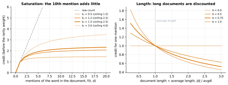
Reading it: on the left, the x-axis is how often a word appears in a document and the y-axis is the credit BM25 gives it (before the rarity weight). The dashed line is raw counting, where 20 mentions count 20 times as much as one. The BM25 curves bend over and flatten toward k₁ + 1: the tenth mention adds almost nothing, which stops keyword-stuffed pages from winning. Smaller k₁ flattens sooner. On the right, one mention in documents of different lengths: with b = 0 length is ignored; with b = 0.75 a mention in a document twice the average length counts noticeably less.
In code: BM25 precomputes each word's IDF and each document's length;
BM25.scores applies the formula to every document, and BM25.search
returns the top k with a non-zero score.
Why it matters: BM25 is decades old, needs no training, runs on any search engine (Elasticsearch, OpenSearch, Lucene), and is still very hard to beat on exact identifiers: product codes, error numbers, names, ticket IDs. Those are everywhere in company data.
2. Meaning search: dense retrieval with a bi-encoder
The everyday picture. The meaning librarian writes a one-line summary card for every book before anyone asks anything. When your question arrives, they write a summary card for it too and pull the books whose cards are most similar. "Automobile reimbursement" and "car mileage expense" get similar cards even though they share no words.
A tiny worked example. With this repo's toy embedding model
(primer.common.embedder), the query "automobile reimbursement" and the
car-mileage article share zero words, yet their vectors have cosine
similarity of about 0.8, the highest in the collection. "What does ERR-4012
mean", by contrast, puts the right article only 4th: the code is one
blurred word among many, and "what" and "mean" pull the vector elsewhere.
flowchart LR
  subgraph AHEAD["Ahead of time"]
    D[Each document] --> E1[Encoder] --> V[(Document vectors)]
  end
  subgraph NOW["At question time"]
    Q[Question] --> E2[Same encoder] --> QV[Question vector]
  end
  QV --> NN["Nearest vectors<br/>(ann.py)"]
  V --> NN
  NN --> R[Ranked documents]
Reading it: the encoder runs twice, but never on the question and a
document together. That's why it's called a bi-encoder: two separate
encodings. Documents are encoded once, at ingestion. A question costs one
encoding plus a nearest-neighbor lookup (see primer.ml.embeddings.ann),
which takes milliseconds over millions of documents. The price: the model
never sees the question and the document side by side, so it can't check
fine details like "does this passage answer this question, or just share
its topic?".
In code: SearchEngine embeds every document once with
primer.common.embedder.ConceptEmbedder into a
primer.ml.embeddings.ann.FlatIndex; SearchEngine.dense embeds the
question and returns the nearest documents. doc_text decides what gets
indexed: the title plus the body.
Why it matters: dense retrieval handles paraphrases, synonyms and other languages, but it blurs exact tokens. Measure both kinds of queries on your own data before trusting either librarian alone.
3. Hybrid search: reciprocal rank fusion (RRF)
The everyday picture. Ask both librarians for their top-10 lists, then hold a vote. A book earns points for each list it's on, more the higher it sits. Books both librarians rank highly rise to the top. Crucially, you only compare positions, never the librarians' private scoring systems, which aren't on the same scale.
A tiny worked example. With the standard constant k = 60:
| Document | Dense rank | BM25 rank | RRF score |
|---|---|---|---|
| X | 1 | 3 | 1/61 + 1/63 = 0.0164 + 0.0159 = 0.0323 |
| Y | 1 | (absent) | 1/61 = 0.0164 |
X, which both methods like, beats Y, which only one method loves.
flowchart LR
  Q[Question] --> B[BM25 ranking]
  Q --> D[Dense ranking]
  B --> R["For every document:<br/>add 1/(60 + rank)<br/>from each list it's on"]
  D --> R
  R --> O[Sort by total:<br/>the fused ranking]
Reading it: the two rankings are the only inputs; their raw scores are thrown away on purpose. BM25 scores run from 0 to about 20; cosine similarities from −1 to 1. Adding them would let one system drown the other, and fixing that needs tuning per collection. Ranks are always on the same scale, so RRF works out of the box.
Level 3: the formula and its symbols
$$ \text{RRF}(d) = \sum_{i=1}^{m} \frac{1}{k + \text{rank}_i(d)} $$
Symbols
| Symbol | Meaning here | Range / typical |
|---|---|---|
| d | a document | |
| m | number of rankings being fused | 2 here (BM25 and dense) |
| i | which ranking | 1 … m |
| rank_i(d) | d's position in ranking i (1 = top); lists d isn't on contribute nothing | 1, 2, 3, … |
| k | a damping constant: keeps rank 1 from dwarfing rank 2 | 60 (from the original paper) |
| RRF(d) | the fused score | small positive numbers |
In words: a document's fused score is the sum, over each ranking it appears in, of one over sixty-plus-its-rank.
On the example: X: 1/(60+1) + 1/(60+3) = 0.01639 + 0.01587 = 0.0323. Y: 1/(60+1) = 0.0164.
Level 3: in Python
In Python:
k = 60
# d's position in each ranking that contains it
def RRF(ranks):
    # Σ_i 1/(k + rank_i(d))
    return sum(1 / (k + rank_i) for rank_i in ranks)
# X: 1st in one ranking, 3rd in the other
round(RRF([1, 3]), 4)  # → 0.0323
# Y: on one ranking only
round(RRF([1]), 4)  # → 0.0164
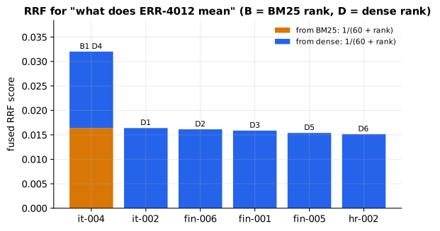
Reading it: each bar is one document's fused score, split into the part contributed by BM25 (orange) and by dense search (blue). The error-code article it-004 is BM25's only hit and dense search's 4th, and the two contributions stack up to put it clearly first. The password-policy article that dense search wrongly ranked first gets only its blue half.
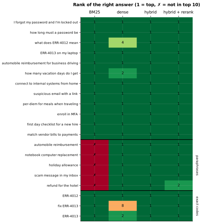
Reading it: one row per question, one column per method; the number is the rank at which the right answer appeared (✗ = not in the top 10). Look at where the colors differ. BM25's failures (the paraphrase block) are where dense search succeeds, and dense search's failures (the error-code block) are where BM25 succeeds. Because their mistakes don't overlap, fusing them fixes both: the hybrid column is all 1s.
| Method | recall@3 (20 questions) | MRR |
|---|---|---|
| BM25 alone | 0.75 | 0.75 |
| Dense alone | 0.90 | 0.85 |
| Hybrid (RRF) | 1.00 | 1.00 |
In code: reciprocal_rank_fusion adds up 1/(k + rank) across any number
of rankings; SearchEngine.hybrid fuses SearchEngine.bm25 with
SearchEngine.dense, and evaluate measures recall@k and MRR for any search
method.
Why it matters: company data is full of both paraphrase-style questions and exact identifiers, so hybrid search almost always beats either method alone. It's cheap to add: most search engines and vector databases support it built in.
4. Reranking: bi-encoder vs. cross-encoder
The everyday picture. A matchmaker has two ways to work. The fast way: write an index card for each person once, then match cards, so thousands of people can be pre-filed. The careful way: sit the two people down together and watch them talk. That's far more accurate, but every pair needs its own meeting. A bi-encoder is the index card. A cross-encoder is the meeting. So you use cards to shortlist, then hold meetings only with the shortlist.
A tiny worked example: a hard negative. "What are the password rules?" has two candidate answers on the same topic. The password reset how-to (it-001) mentions "password" three times; the password policy (it-002) is the real answer. BM25 and the fused hybrid ranking both put the how-to first. A hard negative is exactly this: a document that looks relevant (right topic) but doesn't answer the question.
Our toy cross-encoder reads the question and the document together and checks which of the question's ideas the document covers:
| question ideas: {password, rules} | coverage | phrase | exact | score | |
|---|---|---|---|---|---|
| it-002 policy | password ✓, policy/rules ✓ | 2/2 = 1.0 | 1.0 | 0.5 | ≈ 1.78 |
| it-001 reset how-to | password ✓, rules ✗ | 1/2 = 0.5 | 0.0 | 0.5 | ≈ 0.69 |
The score weighs the features: coverage + 0.5 × phrase + 0.25 × exact + 0.25 × cosine, where the cosine is the ordinary bi-encoder similarity (0.63 for the policy, 0.27 for the how-to). For the policy that's 1.0 + 0.5 + 0.125 + 0.16 ≈ 1.78; for the how-to, 0.5 + 0 + 0.125 + 0.07 ≈ 0.69. After reranking, the policy is first.
flowchart TB
  subgraph BI["Bi-encoder: two separate encodings"]
    direction LR
    Q1[Question] --> EQ[Encoder] --> VQ[vector]
    D1[Document] --> ED[Encoder] --> VD[vector]
    VQ --> COS[cosine]
    VD --> COS
  end
  subgraph CROSS["Cross-encoder: one joint reading"]
    direction LR
    QD["[Question] + [Document]<br/>as one input"] --> J["Encoder with attention<br/>across both texts"] --> SC[relevance score]
  end
Reading it: in the top box, the question and the document never meet
until their vectors are compared, so document vectors can be computed ahead
of time. In the bottom box they're one input, so attention (see
primer.ml.attention) can connect every question word to every document
word: "rules" can notice that the document says "policy" and "must". Nothing
can be precomputed, because the score depends on the pair.
The cost argument. Say a cross-encoder pass takes 10 ms on a GPU. Over a 1-million-document collection that's 10,000 seconds per question. Over a shortlist of 50, it's 0.5 s, or much less when the pairs are batched. That is why the standard pipeline is retrieve wide and cheap, then rerank narrow and precise, and why you cap the shortlist to keep latency predictable.
In code: CrossEncoder.score reads one question-document pair and adds
CrossEncoder.coverage, CrossEncoder.phrase and CrossEncoder.exact, with
ideas grouping synonyms into ideas. retrieve_then_rerank shortlists with
hybrid search, then reorders the shortlist with the cross-encoder.
Why it matters, and a warning: rerankers are models too, and can be wrong. On this repo's 20 questions, reranking fixes the hard negatives but demotes one answer ("refund for the hotel" → it prefers the car-mileage article, which talks about reimbursing trips). Measure recall@k and MRR with and without the reranker before shipping it.
5. Late interaction: ColBERT
The everyday picture. Instead of one summary card per book, keep a card for every word in the book. When your question arrives, each of your words looks for its single best-matching card in the book, and the book's score is how well your words found partners. That's more precise than one summary per book, and unlike the matchmaker's meetings, the cards can still be written ahead of time.
A tiny worked example. Two-number word vectors. The query has words (1, 0) and (0, 1); the document has words (1, 0) and (0.6, 0.8).
| Query word | vs. doc word 1 | vs. doc word 2 | best |
|---|---|---|---|
| (1, 0) | 1.0 | 0.6 | 1.0 |
| (0, 1) | 0.0 | 0.8 | 0.8 |
Score = 1.0 + 0.8 = 1.8.
flowchart LR
  QT["Query: one vector<br/>per word"] --> SIM["Similarity of every<br/>query word × doc word"]
  DT["Document: one vector<br/>per word (precomputed)"] --> SIM
  SIM --> MAX["Each query word keeps<br/>its best match (max)"]
  MAX --> SUM["Add the maxima"] --> S[Score]
Reading it: the grid in the middle is the question-by-document table from the worked example; "max" picks the best cell in each row; "sum" adds the row winners. The document side is precomputed, as with a bi-encoder, but nothing is squeezed into one vector, so each question word gets matched on its own.
Level 3: the formula and its symbols
$$ \text{score}(q, d) = \sum_{i=1}^{|q|} \max_{j=1}^{|d|} \; q_i \cdot d_j $$
Symbols
| Symbol | Meaning here |
|---|---|
| |q|, |d| | number of word vectors in the query and the document |
| q_i | the vector of query word i |
| d_j | the vector of document word j |
| q_i · d_j | dot product: how similar those two words are |
| max over j | the best-matching document word for query word i |
| Σ over i | add those best matches up |
In words: for each query word, find its most similar word in the document, and add up those best similarities.
On the example: max(1.0, 0.6) + max(0.0, 0.8) = 1.0 + 0.8 = 1.8.
Level 3: in Python
In Python:
# one vector per query word
q = [(1, 0), (0, 1)]
# one vector per document word
d = [(1, 0), (0.6, 0.8)]
def dot(a, b):
    return sum(a_k * b_k for a_k, b_k in zip(a, b))
# each query word's best match
[max(dot(q_i, d_j) for d_j in d) for q_i in q]  # → [1, 0.8]
# Σ_i max_j q_i · d_j
sum(max(dot(q_i, d_j) for d_j in d) for q_i in q)  # → 1.8
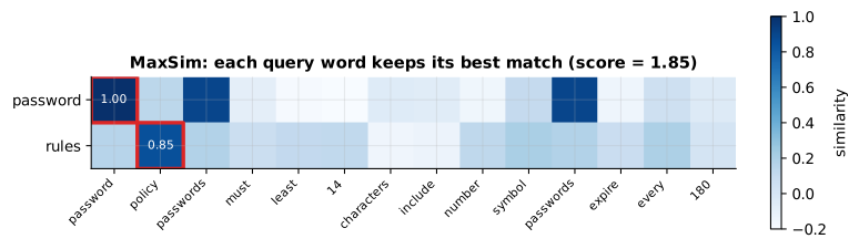
Reading it: rows are the query's words, columns the document's words, and color is the similarity of each pair. The outlined cell in each row is that row's maximum, the only number that counts. "password" finds itself (1.00), ignoring the near-identical "passwords"; "rules" finds "policy" (0.85), a synonym it could never match by spelling. The score is the sum of the outlined cells: 1.00 + 0.85 = 1.85.
In code: maxsim computes the score from two sets of word vectors;
LateInteraction.token_vectors gives a text one vector per word, and
LateInteraction.search ranks documents by MaxSim.
Why it matters: late interaction gets much of a cross-encoder's precision while keeping precomputed documents. The cost is storage: one vector per word instead of per document, often 50 to 200 times more. ColBERTv2 compresses those vectors to make it practical.
6. Chunking: how documents are cut before indexing
The everyday picture. You're turning a cookbook into index cards. Cut every 50 words and a recipe's title lands on one card and its oven temperature on the next. Nobody searching for that recipe finds the temperature. Cut at each recipe instead, and every card is self-contained.
A tiny worked example. A 130-word text, 50-word chunks with 10 words of overlap: windows start every 50 − 10 = 40 words, at 0, 40 and 80, giving 3 chunks (words 1–50, 41–90, 81–130). Each shares 10 words with the next, so a sentence cut at a boundary survives whole in at least one chunk, if it's short.
On this lesson's remote-work handbook, the question "home internet stipend" shows the difference. With 40-word fixed chunks, the best-matching chunk holds the heading "Home internet stipend" but the amount, "50 dollars per month", fell into the next window. With structure-aware chunks, cut at headings, the best chunk holds both.
flowchart LR
  DOC[Document] --> P[Parse: headings,<br/>paragraphs, tables]
  P --> SPLIT["Split at structure;<br/>merge small pieces<br/>up to a size limit"]
  SPLIT --> CTX["Prefix each chunk with<br/>its heading (context)"]
  CTX --> META["Attach metadata: source,<br/>section, date, access list"]
  META --> EMB[Embed + index]
Reading it: chunking is a small pipeline, not a single split. Parsing
decides what the structure is (and is where most quality is lost on messy
PDFs). Splitting respects that structure. Prefixing the heading means a
chunk that says "The stipend is 50 dollars" still says which stipend: the
idea behind contextual retrieval. Metadata rides along so later stages can
filter by date or by who's allowed to see it (see primer.agents.rag).
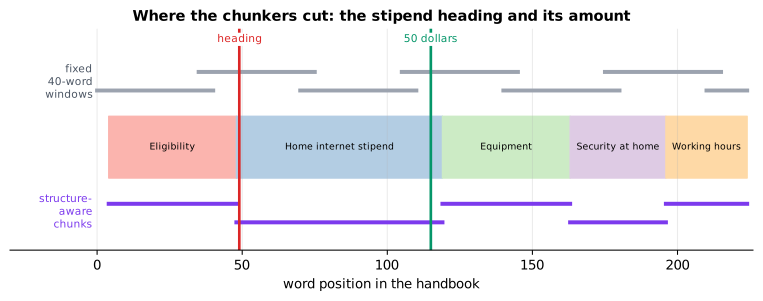
Reading it: the colored strip in the middle is the handbook, one color per section, read left to right by word position. The brackets above it are the fixed 40-word windows; those below are the structure-aware chunks. The red marker is the "Home internet stipend" heading and the green marker the "50 dollars" amount. Above the strip they sit in different windows; below it, one chunk spans both. Notice also that the fixed windows cut straight through section boundaries.
Try it: the handbook below is cut by fixed_size_chunks, then searched
with hybrid search and reranked with the cross-encoder from section 4. With
the stipend question and 40-word chunks, retrieval ranks chunk 2 (the
heading) first, and reranking lifts chunk 3, which holds the amount. Now pick
the VPN question at 30 words with no overlap: the answer sentence is cut
across chunks 6 and 7; raise the overlap to 10 words and one chunk holds it
whole again. Drag top k down to 1 and watch the reranker lose its chance to
help.
Parent-child retrieval. Small chunks match precisely; big chunks give the model enough context. Get both: index small children (single sentences), and when one matches, hand the model its parent (the whole section).
flowchart LR
  Q[Question] --> C["Search small children<br/>(sentences)"]
  C --> HIT[Best child]
  HIT --> PARENT["Look up its parent<br/>(the whole section)"]
  PARENT --> LLM[Give the parent<br/>to the model]
Reading it: the search happens on the left, at sentence level, where matches are sharp. The answer handed on happens on the right, at section level, where context is complete. The lookup in the middle is just a dictionary from child to parent.
Level 3: the formula and its symbols
$$ \text{number of chunks} = \left\lceil \frac{n - o}{s - o} \right\rceil $$
Symbols
| Symbol | Meaning here |
|---|---|
| n | words in the document |
| s | chunk size in words |
| o | overlap in words (smaller than s) |
| s − o | the step: how far each window moves |
| ⌈ ⌉ | "ceiling": round up to a whole number |
In words: the number of chunks is the words left after the first overlap, divided by the step, rounded up.
On the example: ⌈(130 − 10)/(50 − 10)⌉ = ⌈120/40⌉ = 3.
Level 3: in Python
In Python:
import math
# words, chunk size, overlap
n, s, o = 130, 50, 10
# ⌈(n - o) / (s - o)⌉: the step is s - o
math.ceil((n - o) / (s - o))  # → 3
In code: fixed_size_chunks cuts overlapping windows of words;
structure_aware_chunks cuts at headings and paragraphs and returns Chunk
records that carry their heading and metadata. best_chunk picks the chunk
BM25 ranks highest, and parent_child_search matches a sentence and returns
its whole section. chunk_engine indexes one document's chunks so that
retrieve_then_rerank runs on them, as in the widget above.
Why it matters: chunking choices often matter more than the choice of embedding model. Split on structure, keep headings with their content, add modest overlap, and attach metadata for filtering.
7. Asymmetric retrieval and the forgotten prefix
The everyday picture. A filing clerk was trained on sheets stamped "QUESTION:" or "DOCUMENT:", and files each kind in a matching drawer. Hand them an unstamped sheet and they don't complain: they file it anyway, in a drawer nobody will look in. Nobody notices until people stop finding things.
Questions are short and phrased as asks; passages are long statements. Some
embedding models (the E5 family, for example) are trained to expect a
"query: " prefix on questions and a "passage: " prefix on documents, so
they can encode each side appropriately. Forget a prefix and every vector
still looks normal (right length, plausible scores) but sits in a slightly
wrong part of the space.
A tiny worked example. This lesson simulates such a model. With both prefixes, 11 of the 12 everyday questions find their answer in the top 3. Index the documents without "passage: " and the same questions fall to 9 of 12, and MRR drops from 0.875 to about 0.57. No error is raised anywhere.
flowchart LR
  subgraph OK["Correct"]
    Q1["'query: ' + question"] --> E1[Model] --> A1[aligned vectors]
    D1["'passage: ' + document"] --> E1
  end
  subgraph BUG["Prefix forgotten at indexing"]
    Q2["'query: ' + question"] --> E2[Model] --> A2[question vectors]
    D2["document (no prefix)"] --> E2 --> B2[drifted document vectors]
  end
Reading it: the top box is how the model was trained: both sides stamped, vectors aligned. In the bottom box the documents were indexed unstamped. The model still returns vectors, and the pipeline runs, but the two sides no longer line up well. The only way to catch it is to measure recall on labeled questions, which is the habit this whole lesson argues for.
In code: PrefixedEmbedder simulates such a model:
PrefixedEmbedder.encode_one strips a known prefix and encodes normally, but
partly rotates the vector of any text that lacks one.
Why it matters: always read the embedding model's card for required prefixes or instructions, use the same model and settings at indexing and query time, and keep a small labeled set so silent regressions show up.
In 20 seconds
- BM25 scores keyword matches: rare words weigh more (IDF), repeated mentions saturate (k₁), long documents are discounted (b). It's great at exact IDs and blind to synonyms.
- Dense retrieval (bi-encoder) finds meaning and paraphrases, but blurs exact tokens. Documents are embedded once, ahead of time.
- Hybrid search fuses both rankings with RRF, Σ 1/(60 + rank), using ranks not scores, and almost always beats either alone.
- Retrieve, then rerank: a bi-encoder or hybrid search shortlists 50 to 100 cheaply; a cross-encoder reads each (question, candidate) pair together and reorders the shortlist precisely.
- ColBERT keeps a vector per word and scores with MaxSim: close to cross-encoder precision, still precomputable, much more storage.
- Chunk on structure, keep headings with content, attach metadata, and measure recall@k on labeled questions: it's how you catch silent bugs like a forgotten prefix.
Self-test questions
Documents "cat cat dog", "dog bird", "fish"; query "cat". What does BM25 give the first document? IDF(cat) = ln(1 + 2.5/1.5) = 0.981. With f = 2, |d| = 3, avgdl = 2, k₁ = 1.5 and b = 0.75 the denominator is 2 + 1.5 · 1.375 = 4.0625, so the score is 0.981 · 2 · 2.5 / 4.0625 = 1.207.
A document is 1st in dense search and 3rd in BM25. What's its RRF score? 1/61 + 1/63 ≈ 0.0323, versus 0.0164 for a document that is 1st in only one list.
Query words (1, 0) and (0, 1); document words (1, 0) and (0.6, 0.8). What's the MaxSim score? max(1.0, 0.6) + max(0.0, 0.8) = 1.8.
How many 50-word chunks with 10 words of overlap does a 130-word text make? ⌈(130 − 10)/(50 − 10)⌉ = 3, starting at words 0, 40 and 80.
What goes wrong if you forget an embedding model's "passage: " prefix when indexing? Nothing errors: vectors look normal and scores look plausible, but documents land where the model never aligned them with questions, and recall silently drops (11 of 12 to 9 of 12 in the lesson's simulation). Only an evaluation on labeled questions catches it.
What do BM25's k₁ and b control? k₁ sets saturation: how fast extra mentions of a word stop adding score (the credit per word can never exceed k₁ + 1). b sets length normalization: 0 ignores document length, 1 fully scales mentions by length relative to the average. Typical values are k₁ ≈ 1.2 to 2 and b = 0.75.
Bi-encoder vs. cross-encoder: how do you combine them in one pipeline? A bi-encoder embeds questions and documents separately, so documents are embedded once and searched in milliseconds with an ANN index; it's fast but never sees the pair together. A cross-encoder reads question and document as one input, so it's accurate but costs one model pass per pair and can't precompute anything. Combine them: retrieve the top 50 to 100 with the bi-encoder (or hybrid search), rerank that shortlist with the cross-encoder, and pass the top few to the model. Cap the shortlist to keep latency predictable.
Why does hybrid search beat pure vector search on company data? Company data is full of exact identifiers (error codes, product SKUs, ticket numbers, names) that embeddings blur, and full of paraphrases and jargon that keyword search misses. BM25 and dense search fail on different questions, so fusing their rankings with RRF recovers the answers each one misses.
Why does RRF use ranks instead of scores? BM25 scores and cosine similarities live on unrelated scales, and those scales vary by query and collection. Ranks are always comparable, so RRF needs no tuning or score normalization. The constant k = 60 keeps the very top rank from dominating.
What's a hard negative, and how do you fix one in retrieval?
A document on the right topic that doesn't answer the question, like the
password-reset how-to for "what are the password rules". Fix it with a
reranker that reads the question and document together, and when you
fine-tune an embedding model, train on hard negatives so it learns the
distinction (see primer.ml.embeddings.contrastive).
What does ColBERT trade to get better precision than a bi-encoder? Storage and some query cost. It keeps one vector per word instead of one per document, often 50 to 200 times more vectors, and scores with MaxSim over word pairs, in exchange for word-level matching with precomputed documents.
Fixed-size vs. structure-aware chunking? Fixed-size windows are simple but cut through headings, sentences and tables, separating facts from their context. Structure-aware chunking splits at headings and paragraphs, keeps each heading with its content, and attaches metadata. Parent-child retrieval searches small pieces but returns their larger parent for context.
Your RAG system gives confident wrong answers. How do you tell whether retrieval is the cause? Build a small labeled set of real questions with known answer passages and measure recall@k of retrieval alone. If the right passage isn't in the top k, no prompt change will fix the answer; fix retrieval (hybrid, reranking, chunking, prefixes, domain fine-tuning). If it is there, the problem is in generation.
The papers behind this lesson
- Robertson & Zaragoza, The Probabilistic Relevance Framework: BM25 and Beyond (Foundations and Trends in Information Retrieval, 2009). https://www.nowpublishers.com/article/Details/INR-019. The authoritative account of where BM25 comes from: the probabilistic model behind IDF, and why term-frequency saturation and length normalization take the form they do.
- Cormack, Clarke & Büttcher, Reciprocal Rank Fusion outperforms Condorcet and individual Rank Learning Methods (SIGIR 2009). https://plg.uwaterloo.ca/~gvcormac/cormacksigir09-rrf.pdf. Introduced RRF, Σ 1/(k + rank) with k = 60, and showed that this simple, tuning-free fusion beats more elaborate methods.
- Reimers & Gurevych, Sentence-BERT (2019). https://arxiv.org/abs/1908.10084. Made bi-encoders practical: a siamese BERT that produces one comparable vector per sentence, turning hours of pairwise cross-encoding into milliseconds of vector search. annotated companion
- Karpukhin et al., Dense Passage Retrieval for Open-Domain Question Answering (2020). https://arxiv.org/abs/2004.04906. Showed a dual encoder trained with in-batch and BM25-mined hard negatives can beat BM25 on open-domain question answering, the template for modern dense retrievers. annotated companion
- Khattab & Zaharia, ColBERT: Efficient and Effective Passage Search via Contextualized Late Interaction over BERT (2020). https://arxiv.org/abs/2004.12832. Introduced late interaction: per-token vectors scored with MaxSim, getting near cross-encoder quality with precomputed documents. annotated companion
Further reading
- Nogueira & Cho, Passage Re-ranking with BERT (2019), the cross-encoder reranker: https://arxiv.org/abs/1901.04085
- Santhanam et al., ColBERTv2 (compressed late interaction): https://arxiv.org/abs/2112.01488
- Wang et al., Text Embeddings by Weakly-Supervised Contrastive Pre-training (E5, the query/passage prefixes): https://arxiv.org/abs/2212.03533
- Anthropic, Introducing Contextual Retrieval (contextual chunk prefixes + hybrid + reranking): https://www.anthropic.com/news/contextual-retrieval
- sentence-transformers documentation (bi-encoders and cross-encoders): https://www.sbert.net/
- Elasticsearch reciprocal rank fusion reference: https://www.elastic.co/guide/en/elasticsearch/reference/current/rrf.html
1r""" 2# Retrieval: keyword search, meaning search, and combining them 3 4Run: `python -m primer.ml.embeddings.retrieval` 5 6New to the notation (Σ, log, |d|)? `primer.notation` explains every symbol 7used here from zero. 8 9## Level 1: The practitioner's guide 10 11**In one sentence.** Retrieval finds the few passages that answer a 12question, ranked best first, by running a keyword search and a meaning 13search side by side, fusing their rankings, and letting a slower, more 14careful model reorder the short list that survives. 15 16**When you need it.** You need retrieval whenever a model must answer from 17material it was not trained on and that material is too big to paste into 18the prompt: a knowledge base of tickets, manuals, contracts or code. 19Anthropic's contextual retrieval post puts the line at about 200,000 tokens 20(about 500 pages): below that, put the whole knowledge base in the prompt 21and skip retrieval. Above it, retrieval quality caps answer quality, because 22the language model can only use what retrieval hands it (`primer.agents.rag`). 23The tell that one search method is not enough: on this lesson's 20 labeled 24questions, keyword search alone puts the answer in the top 3 for 75% of them 25and meaning search alone for 90%, and their misses never overlap. Keyword 26search fails on paraphrases ("automobile reimbursement" when the document 27says "car" and "reimbursed"); meaning search puts the article for "ERR-4012" 28fourth. Fused, they reach 100%. 29 30**Your options.** From the cheapest to the most precise; in practice each 31stage feeds the next: 32 33| Option | What it does | What it gives you | What it costs | Where it lives | 34|---|---|---|---|---| 35| Keyword search (BM25) | Weighs each query word by rarity, saturates repeated mentions, discounts long documents | Exact matches on identifiers, codes and names, with no training | Nothing for synonyms: a document sharing no words scores 0 | Lucene, Elasticsearch, OpenSearch, any search engine | 36| Dense retrieval (bi-encoder) | Embeds every document once and the question at query time, then returns the nearest vectors | Paraphrases, synonyms, other languages | An embedding model and a vector index; exact tokens blur | An embedding model plus a vector index (`primer.ml.embeddings.ann`) | 37| Hybrid search (RRF) | Runs both and fuses the two rankings by position, never by score | The strengths of both, with no tuning | Two searches per query and a merge | Built into Elasticsearch and most vector databases | 38| Reranking (cross-encoder) | Reads the question and each shortlisted candidate together and reorders them | Catches hard negatives: right topic, wrong answer | One model pass per candidate, so it only ever sees a shortlist | sentence-transformers cross-encoders, Cohere Rerank | 39| Late interaction (ColBERT) | Keeps one vector per word and matches each question word to its best document word | Near cross-encoder precision with precomputed documents | 50 to 200 times the vector storage | ColBERT and ColBERTv2 | 40 41**How to choose.** Start from what your questions look like and how much 42latency you can spend. 43 44- Questions full of identifiers (error codes, product codes, ticket 45 numbers, names): keyword search is hard to beat and must be in the 46 pipeline. Company data is full of these. 47- Questions phrased differently from the documents (paraphrases, jargon, 48 other languages): dense retrieval. Read the model card for required 49 prefixes (`query: ` and `passage: ` for the E5 family) and use the same 50 model and settings at indexing and query time. 51- Almost always: both, fused with reciprocal rank fusion at its standard 52 constant of 60. It is cheap, needs no tuning, and on this lesson's 53 questions lifts recall@3 from 0.75 and 0.90 to 1.00. 54- When the top results are on the right topic but don't answer the question 55 (a password *reset* guide above the password *policy*): add a reranker 56 over a shortlist of 50 to 100, and measure recall and MRR with and without 57 it. Rerankers can demote a right answer too: this lesson's fixes the hard 58 negative and lowers MRR from 1.00 to 0.975 on the same 20 questions. 59- When one vector per document is too coarse and you can afford the 60 storage: late interaction. 61- Whatever you pick, decide the chunking first: split on structure, keep 62 headings with their content, add modest overlap, attach metadata. It often 63 matters more than the choice of embedding model. Then keep a small labeled 64 set of questions with known answer passages and measure recall@k on it. 65 66**What it costs.** Keyword and dense search are the cheap, wide stages: 67documents are indexed once, and a question costs one embedding plus a 68lookup that takes milliseconds over millions of documents. Fusion is a merge 69of two short lists. The reranker is where money and latency go: at 10 ms per 70pair on a GPU, scoring a million documents takes 10,000 seconds, and a 71shortlist of 50 takes 0.5 s (less when the pairs are batched), which is why 72the shortlist is capped. Late interaction trades that latency for storage: 73one vector per word instead of one per document. Preparing the chunks has a 74price too: Anthropic reports \$1.02 per million document tokens, once, to 75write a short context in front of every chunk with prompt caching, for a 49% 76cut in top-20 retrieval failures with hybrid search and a 67% cut with 77reranking added (from 5.7% to 1.9% on their evaluation). The cheapest item 78of all, and the one most teams skip, is a labeled set of a few dozen 79questions with known answer passages: it is the only instrument that shows 80the failures below. 81 82**What breaks.** 83 84- **The right page is never found.** If the passage is not in the top k, no 85 prompt change will fix the answer. Measure recall@k of retrieval alone 86 before touching the prompt. 87- **A forgotten prefix.** Index documents without the `passage: ` prefix a 88 model was trained with and nothing errors: vectors look normal, scores 89 look plausible, and in this lesson's simulation recall@3 falls from 0.92 90 to 0.75 and MRR from 0.875 to 0.57. Only a labeled set catches it. 91- **Scores added across systems.** BM25 scores run from 0 to about 20 and 92 cosine similarities from −1 to 1; add them and one system drowns the 93 other. Fuse ranks, not scores. 94- **Hard negatives.** A document on the right topic that doesn't answer the 95 question rises because it shares the words. A reranker reads the pair 96 together; when you fine-tune an embedding model, train it on such pairs 97 (`primer.ml.embeddings.contrastive`). 98- **A heading cut from its fact.** Fixed 40-word windows split the heading 99 "Home internet stipend" from "50 dollars per month" in this lesson's 100 handbook; a structure-aware chunk holds both. Parent-child retrieval 101 searches small children and returns their whole section. 102- **A reranker trusted blindly.** It is a model and can be wrong: this 103 lesson's demotes one correct answer while fixing another. Ship it only 104 when the numbers say so. 105- **A shortlist too short.** Give the reranker only the top result and it 106 cannot help. Anthropic's evaluation retrieved 150 chunks, reranked them 107 to 20, and found that passing 20 chunks to the model beat passing 10 or 5. 108 109**In the wild.** BM25 runs in any search engine: Lucene, Elasticsearch, 110OpenSearch. Elasticsearch's `rrf` retriever fuses a BM25 query with a kNN 111query by the same one-over-sixty-plus-rank rule (`rank_constant` 60 by 112default) with no weights to tune. Bi-encoders trace back to Sentence-BERT 113and Dense Passage Retrieval; the sentence-transformers library ships both 114bi-encoders and cross-encoder rerankers, and hosted rerankers such as Cohere 115Rerank take a query and a list of documents and return them ordered by 116relevance, cut to a `top_n`. Cross-encoder reranking with BERT is due to 117Nogueira and Cho, late interaction to ColBERT and ColBERTv2, and the E5 118models are the ones trained with the `query: ` and `passage: ` prefixes. 119Anthropic's contextual retrieval puts a generated context in front of every 120chunk and combines it with hybrid search and reranking. The papers behind 121this lesson are listed at the end with their companions. 122 123**Go deeper.** Level 2 builds every box of the pipeline by hand: BM25 on 124three one-line documents, the bi-encoder over this repo's toy embedder, 125reciprocal rank fusion on two ranks, a toy cross-encoder scoring a hard 126negative, ColBERT's MaxSim on two-number word vectors, the chunking 127arithmetic, and the forgotten-prefix bug measured. If you only needed to 128design the pipeline, you are done. 129 130## Level 2: How it works, from scratch 131 132Level 2 builds every box of that pipeline from nothing, starting in a 133library. 134 135**The everyday picture.** You walk into a library with a question. Two librarians are on duty. 136 137- **The keyword librarian** takes your words literally. They count how often 138 each word of your question appears in each book, give *rare* words far more 139 weight than common ones, stop getting more excited after the tenth mention, 140 and are a little suspicious of very long books that mention everything. 141 Ask about "ERR-4012" and they find the one page that says "ERR-4012". Ask 142 about "automobile reimbursement" and they find nothing, because the book 143 says "car" and "reimbursed". 144- **The meaning librarian** understands what you *mean*: "automobile" is a 145 "car", "scam" is "phishing". But they remember the gist of each book, not 146 its serial numbers, so "ERR-4012" and "ERR-4013" blur together. 147 148Real systems ask **both** and trust the books both recommend. Then an 149expert reads the top handful of candidates carefully, next to your question, 150and puts them in final order. That's the whole modern retrieval pipeline, 151and this lesson builds every piece of it. 152 153Words used throughout, in plain terms: 154 155- **Retrieval.** Finding the documents that answer a question, ranked best 156 first. In a RAG system (`primer.agents.rag`) the language model can only use 157 what retrieval hands it, so retrieval quality caps answer quality. 158- **Token.** Here, one word after lowercasing and dropping filler words 159 ("the", "is"): see `primer.common.text`. 160- **Recall@k.** The share of questions whose answer appears in the top k 161 results. **MRR** (mean reciprocal rank) also rewards putting the answer 162 *first*: an answer at rank 1 scores 1, at rank 2 scores 1/2, missing scores 163 0, averaged over questions. 164 165The full pipeline, which the sections below build one box at a time: 166 167```mermaid 168flowchart LR 169 Q[Question] --> K[Keyword search<br/>BM25] 170 Q --> D[Meaning search<br/>embeddings] 171 K --> F[Fuse the two rankings<br/>RRF] 172 D --> F 173 F --> S[Shortlist<br/>top 10 to 100] 174 S --> R[Rerank each candidate<br/>with the question: cross-encoder] 175 R --> T[Top 3 to 5 passages<br/>to the language model] 176``` 177 178**Reading it:** two cheap, wide searches run side by side and see the whole 179collection. Their rankings are merged into one shortlist. Only the shortlist 180reaches the expensive, precise reranker on the right. Everything left of the 181shortlist must be fast because it faces millions of documents; everything 182right of it can be slow because it faces only a hundred. Each box below gets 183its own section. 184 185## 1. Keyword search: BM25 186 187**The everyday picture.** The keyword librarian from above: rare words count 188more, repetition helps less and less, and long books get a small penalty for 189mentioning everything. 190 191**A tiny worked example.** Three one-line "documents": 192 193| Doc | Words | Length | 194|---|---|---| 195| d₁ | cat cat dog | 3 | 196| d₂ | dog bird | 2 | 197| d₃ | fish | 1 | 198 199The average length is (3 + 2 + 1)/3 = 2. Search for **cat**. It appears in 200one of the three documents, so it's rare and gets a high weight (0.981, 201computed below); "dog" is in two, so it would get less (0.470). Only d₁ 202contains "cat", twice, and d₁ is a bit longer than average. Plugging in, 203d₁ scores **1.207** and the others score 0. 204 205```mermaid 206flowchart LR 207 Q[Query words] --> IDF["Rarity weight per word<br/>IDF: rarer = heavier"] 208 Q --> TF["Count in this document<br/>tf, with saturation"] 209 DL["Document length vs.<br/>the average length"] --> TF 210 IDF --> M((×)) 211 TF --> M 212 M --> SUM["Add up over<br/>the query's words"] 213 SUM --> S[BM25 score] 214``` 215 216**Reading it:** each query word contributes one product: *how rare the word 217is* times *how much this document talks about it*. The length box feeds into 218the count box because a mention in a short document is stronger evidence than 219the same mention in a long one. Words the document doesn't contain 220contribute zero, so a document sharing no words with the query scores exactly 2210. That's the blind spot the meaning librarian covers. 222 223$$ 224\text{BM25}(q, d) = \sum_{t \in q} \text{IDF}(t) \cdot 225\frac{f(t, d)\,(k_1 + 1)}{f(t, d) + k_1 \left(1 - b + b\,\frac{|d|}{\text{avgdl}}\right)}, 226\qquad 227\text{IDF}(t) = \ln\!\left(1 + \frac{N - n(t) + 0.5}{n(t) + 0.5}\right) 228$$ 229 230**Symbols** 231 232| Symbol | Meaning here | Range / typical | 233|---|---|---| 234| q | the query, as a list of words | | 235| d | one document, as a list of words | | 236| t ∈ q | "each word t in the query" | | 237| Σ | add up the following over every query word | | 238| f(t, d) | how many times word t appears in document d (term frequency) | 0, 1, 2, … | 239| \|d\| | the document's length in words | | 240| avgdl | the average document length in the collection | | 241| k₁ | saturation: how quickly extra mentions stop helping | 1.2 to 2.0; 1.5 here | 242| b | length normalization: 0 ignores length, 1 fully normalizes | 0.75 | 243| N | number of documents in the collection | | 244| n(t) | number of documents containing t (document frequency) | 1 … N | 245| ln | natural logarithm: grows slowly, so ten times rarer is not ten times heavier | | 246| IDF(t) | inverse document frequency: the word's rarity weight | ≥ 0 | 247 248**In words:** for each word of the query, multiply how rare the word is by a 249count of its mentions that saturates and is adjusted for document length, 250then add those products up. 251 252**On the example (query "cat", document d₁):** N = 3, n(cat) = 1, so 253IDF = ln(1 + 2.5/1.5) = ln(2.667) = **0.981**. f = 2, |d| = 3, avgdl = 2: 254the denominator is 2 + 1.5 · (1 − 0.75 + 0.75 · 3/2) = 2 + 1.5 · 1.375 = 2554.0625. The count part is 2 · 2.5 / 4.0625 = 1.231. Score = 0.981 · 1.231 = 256**1.207**. 257 258**In Python:** 259 260```python 261import math 262# 3 documents; 1 of them contains "cat" 263N, n_t = 3, 1 264# ln(1 + (N - n(t) + 0.5) / (n(t) + 0.5)) 265IDF = math.log(1 + (N - n_t + 0.5) / (n_t + 0.5)) 266round(IDF, 3) # → 0.981 267# f(cat, d1), |d1|, average document length 268f, d_len, avgdl = 2, 3, 2 269k_1, b = 1.5, 0.75 270count_part = f * (k_1 + 1) / (f + k_1 * (1 - b + b * d_len / avgdl)) 271round(count_part, 3) # → 1.231 272# Σ over the query's only word 273round(IDF * count_part, 3) # → 1.207 274``` 275 276 277 278**Reading it:** on the left, the x-axis is how often a word appears in a 279document and the y-axis is the credit BM25 gives it (before the rarity 280weight). The dashed line is raw counting, where 20 mentions count 20 times 281as much as one. The BM25 curves bend over and flatten toward k₁ + 1: the 282tenth mention adds almost nothing, which stops keyword-stuffed pages from 283winning. Smaller k₁ flattens sooner. On the right, one mention in documents 284of different lengths: with b = 0 length is ignored; with b = 0.75 a mention 285in a document twice the average length counts noticeably less. 286 287**In code:** `BM25` precomputes each word's IDF and each document's length; 288`BM25.scores` applies the formula to every document, and `BM25.search` 289returns the top k with a non-zero score. 290 291**Why it matters:** BM25 is decades old, needs no training, runs on any 292search engine (Elasticsearch, OpenSearch, Lucene), and is still very hard to 293beat on exact identifiers: product codes, error numbers, names, ticket IDs. 294Those are everywhere in company data. 295 296## 2. Meaning search: dense retrieval with a bi-encoder 297 298**The everyday picture.** The meaning librarian writes a one-line summary 299card for every book *before* anyone asks anything. When your question 300arrives, they write a summary card for it too and pull the books whose cards 301are most similar. "Automobile reimbursement" and "car mileage expense" get 302similar cards even though they share no words. 303 304**A tiny worked example.** With this repo's toy embedding model 305(`primer.common.embedder`), the query "automobile reimbursement" and the 306car-mileage article share zero words, yet their vectors have cosine 307similarity of about 0.8, the highest in the collection. "What does ERR-4012 308mean", by contrast, puts the right article only 4th: the code is one 309blurred word among many, and "what" and "mean" pull the vector elsewhere. 310 311```mermaid 312flowchart LR 313 subgraph AHEAD["Ahead of time"] 314 D[Each document] --> E1[Encoder] --> V[(Document vectors)] 315 end 316 subgraph NOW["At question time"] 317 Q[Question] --> E2[Same encoder] --> QV[Question vector] 318 end 319 QV --> NN["Nearest vectors<br/>(ann.py)"] 320 V --> NN 321 NN --> R[Ranked documents] 322``` 323 324**Reading it:** the encoder runs twice, but never on the question and a 325document *together*. That's why it's called a **bi-encoder**: two separate 326encodings. Documents are encoded once, at ingestion. A question costs one 327encoding plus a nearest-neighbor lookup (see `primer.ml.embeddings.ann`), 328which takes milliseconds over millions of documents. The price: the model 329never sees the question and the document side by side, so it can't check 330fine details like "does this passage answer *this* question, or just share 331its topic?". 332 333**In code:** `SearchEngine` embeds every document once with 334`primer.common.embedder.ConceptEmbedder` into a 335`primer.ml.embeddings.ann.FlatIndex`; `SearchEngine.dense` embeds the 336question and returns the nearest documents. `doc_text` decides what gets 337indexed: the title plus the body. 338 339**Why it matters:** dense retrieval handles paraphrases, synonyms and other 340languages, but it blurs exact tokens. Measure both kinds of queries on your 341own data before trusting either librarian alone. 342 343## 3. Hybrid search: reciprocal rank fusion (RRF) 344 345**The everyday picture.** Ask both librarians for their top-10 lists, then 346hold a vote. A book earns points for each list it's on, more the higher it 347sits. Books both librarians rank highly rise to the top. Crucially, you only 348compare *positions*, never the librarians' private scoring systems, which 349aren't on the same scale. 350 351**A tiny worked example.** With the standard constant k = 60: 352 353| Document | Dense rank | BM25 rank | RRF score | 354|---|---|---|---| 355| X | 1 | 3 | 1/61 + 1/63 = 0.0164 + 0.0159 = **0.0323** | 356| Y | 1 | (absent) | 1/61 = **0.0164** | 357 358X, which both methods like, beats Y, which only one method loves. 359 360```mermaid 361flowchart LR 362 Q[Question] --> B[BM25 ranking] 363 Q --> D[Dense ranking] 364 B --> R["For every document:<br/>add 1/(60 + rank)<br/>from each list it's on"] 365 D --> R 366 R --> O[Sort by total:<br/>the fused ranking] 367``` 368 369**Reading it:** the two rankings are the only inputs; their raw scores are 370thrown away on purpose. BM25 scores run from 0 to about 20; cosine 371similarities from −1 to 1. Adding them would let one system drown the other, 372and fixing that needs tuning per collection. Ranks are always on the same 373scale, so RRF works out of the box. 374 375$$ 376\text{RRF}(d) = \sum_{i=1}^{m} \frac{1}{k + \text{rank}_i(d)} 377$$ 378 379**Symbols** 380 381| Symbol | Meaning here | Range / typical | 382|---|---|---| 383| d | a document | | 384| m | number of rankings being fused | 2 here (BM25 and dense) | 385| i | which ranking | 1 … m | 386| rank_i(d) | d's position in ranking i (1 = top); lists d isn't on contribute nothing | 1, 2, 3, … | 387| k | a damping constant: keeps rank 1 from dwarfing rank 2 | 60 (from the original paper) | 388| RRF(d) | the fused score | small positive numbers | 389 390**In words:** a document's fused score is the sum, over each ranking it 391appears in, of one over sixty-plus-its-rank. 392 393**On the example:** X: 1/(60+1) + 1/(60+3) = 0.01639 + 0.01587 = **0.0323**. 394Y: 1/(60+1) = **0.0164**. 395 396**In Python:** 397 398```python 399k = 60 400# d's position in each ranking that contains it 401def RRF(ranks): 402 # Σ_i 1/(k + rank_i(d)) 403 return sum(1 / (k + rank_i) for rank_i in ranks) 404# X: 1st in one ranking, 3rd in the other 405round(RRF([1, 3]), 4) # → 0.0323 406# Y: on one ranking only 407round(RRF([1]), 4) # → 0.0164 408``` 409 410 411 412**Reading it:** each bar is one document's fused score, split into the part 413contributed by BM25 (orange) and by dense search (blue). The error-code 414article it-004 is BM25's only hit and dense search's 4th, and the two 415contributions stack up to put it clearly first. The password-policy article 416that dense search wrongly ranked first gets only its blue half. 417 418 419 420**Reading it:** one row per question, one column per method; the number is 421the rank at which the right answer appeared (✗ = not in the top 10). Look at 422where the colors differ. BM25's failures (the paraphrase block) are where 423dense search succeeds, and dense search's failures (the error-code block) are 424where BM25 succeeds. Because their mistakes don't overlap, fusing them fixes 425both: the hybrid column is all 1s. 426 427| Method | recall@3 (20 questions) | MRR | 428|---|---|---| 429| BM25 alone | 0.75 | 0.75 | 430| Dense alone | 0.90 | 0.85 | 431| **Hybrid (RRF)** | **1.00** | **1.00** | 432 433**In code:** `reciprocal_rank_fusion` adds up 1/(k + rank) across any number 434of rankings; `SearchEngine.hybrid` fuses `SearchEngine.bm25` with 435`SearchEngine.dense`, and `evaluate` measures recall@k and MRR for any search 436method. 437 438**Why it matters:** company data is full of both paraphrase-style questions 439and exact identifiers, so hybrid search almost always beats either method 440alone. It's cheap to add: most search engines and vector databases support 441it built in. 442 443## 4. Reranking: bi-encoder vs. cross-encoder 444 445**The everyday picture.** A matchmaker has two ways to work. The fast way: 446write an index card for each person once, then match cards, so thousands of 447people can be pre-filed. The careful way: sit the two people down *together* 448and watch them talk. That's far more accurate, but every pair needs its own 449meeting. A **bi-encoder** is the index card. A **cross-encoder** is the 450meeting. So you use cards to shortlist, then hold meetings only with the 451shortlist. 452 453**A tiny worked example: a hard negative.** "What are the password rules?" 454has two candidate answers on the same topic. The password *reset* how-to 455(it-001) mentions "password" three times; the password *policy* (it-002) is 456the real answer. BM25 and the fused hybrid ranking both put the how-to first. 457A **hard negative** is exactly this: a document that looks relevant (right 458topic) but doesn't answer the question. 459 460Our toy cross-encoder reads the question and the document together and 461checks which of the question's *ideas* the document covers: 462 463| | question ideas: {password, rules} | coverage | phrase | exact | score | 464|---|---|---|---|---|---| 465| it-002 policy | password ✓, policy/rules ✓ | 2/2 = **1.0** | 1.0 | 0.5 | ≈ 1.78 | 466| it-001 reset how-to | password ✓, rules ✗ | 1/2 = **0.5** | 0.0 | 0.5 | ≈ 0.69 | 467 468The score weighs the features: coverage + 0.5 × phrase + 0.25 × exact + 4690.25 × cosine, where the cosine is the ordinary bi-encoder similarity (0.63 470for the policy, 0.27 for the how-to). For the policy that's 1.0 + 0.5 + 4710.125 + 0.16 ≈ 1.78; for the how-to, 0.5 + 0 + 0.125 + 0.07 ≈ 0.69. 472After reranking, the policy is first. 473 474```mermaid 475flowchart TB 476 subgraph BI["Bi-encoder: two separate encodings"] 477 direction LR 478 Q1[Question] --> EQ[Encoder] --> VQ[vector] 479 D1[Document] --> ED[Encoder] --> VD[vector] 480 VQ --> COS[cosine] 481 VD --> COS 482 end 483 subgraph CROSS["Cross-encoder: one joint reading"] 484 direction LR 485 QD["[Question] + [Document]<br/>as one input"] --> J["Encoder with attention<br/>across both texts"] --> SC[relevance score] 486 end 487``` 488 489**Reading it:** in the top box, the question and the document never meet 490until their vectors are compared, so document vectors can be computed ahead 491of time. In the bottom box they're one input, so attention (see 492`primer.ml.attention`) can connect every question word to every document 493word: "rules" can notice that the document says "policy" and "must". Nothing 494can be precomputed, because the score depends on the pair. 495 496**The cost argument.** Say a cross-encoder pass takes 10 ms on a GPU. Over a 4971-million-document collection that's 10,000 seconds per question. Over a 498shortlist of 50, it's 0.5 s, or much less when the pairs are batched. That 499is why the standard pipeline is *retrieve wide and cheap, then rerank narrow 500and precise*, and why you cap the shortlist to keep latency predictable. 501 502**In code:** `CrossEncoder.score` reads one question-document pair and adds 503`CrossEncoder.coverage`, `CrossEncoder.phrase` and `CrossEncoder.exact`, with 504`ideas` grouping synonyms into ideas. `retrieve_then_rerank` shortlists with 505hybrid search, then reorders the shortlist with the cross-encoder. 506 507**Why it matters, and a warning:** rerankers are models too, and can be wrong. 508On this repo's 20 questions, reranking fixes the hard negatives but demotes 509one answer ("refund for the hotel" → it prefers the car-mileage article, 510which talks about reimbursing trips). Measure recall@k and MRR with and 511without the reranker before shipping it. 512 513## 5. Late interaction: ColBERT 514 515**The everyday picture.** Instead of one summary card per book, keep a card 516for *every word* in the book. When your question arrives, each of your words 517looks for its single best-matching card in the book, and the book's score is 518how well your words found partners. That's more precise than one summary per 519book, and unlike the matchmaker's meetings, the cards can still be written 520ahead of time. 521 522**A tiny worked example.** Two-number word vectors. The query has words 523(1, 0) and (0, 1); the document has words (1, 0) and (0.6, 0.8). 524 525| Query word | vs. doc word 1 | vs. doc word 2 | best | 526|---|---|---|---| 527| (1, 0) | 1.0 | 0.6 | **1.0** | 528| (0, 1) | 0.0 | 0.8 | **0.8** | 529 530Score = 1.0 + 0.8 = **1.8**. 531 532```mermaid 533flowchart LR 534 QT["Query: one vector<br/>per word"] --> SIM["Similarity of every<br/>query word × doc word"] 535 DT["Document: one vector<br/>per word (precomputed)"] --> SIM 536 SIM --> MAX["Each query word keeps<br/>its best match (max)"] 537 MAX --> SUM["Add the maxima"] --> S[Score] 538``` 539 540**Reading it:** the grid in the middle is the question-by-document table 541from the worked example; "max" picks the best cell in each row; "sum" adds 542the row winners. The document side is precomputed, as with a bi-encoder, but 543nothing is squeezed into one vector, so each question word gets matched on 544its own. 545 546$$ 547\text{score}(q, d) = \sum_{i=1}^{|q|} \max_{j=1}^{|d|} \; q_i \cdot d_j 548$$ 549 550**Symbols** 551 552| Symbol | Meaning here | 553|---|---| 554| \|q\|, \|d\| | number of word vectors in the query and the document | 555| q_i | the vector of query word i | 556| d_j | the vector of document word j | 557| q_i · d_j | dot product: how similar those two words are | 558| max over j | the best-matching document word for query word i | 559| Σ over i | add those best matches up | 560 561**In words:** for each query word, find its most similar word in the 562document, and add up those best similarities. 563 564**On the example:** max(1.0, 0.6) + max(0.0, 0.8) = 1.0 + 0.8 = **1.8**. 565 566**In Python:** 567 568```python 569# one vector per query word 570q = [(1, 0), (0, 1)] 571# one vector per document word 572d = [(1, 0), (0.6, 0.8)] 573def dot(a, b): 574 return sum(a_k * b_k for a_k, b_k in zip(a, b)) 575# each query word's best match 576[max(dot(q_i, d_j) for d_j in d) for q_i in q] # → [1, 0.8] 577# Σ_i max_j q_i · d_j 578sum(max(dot(q_i, d_j) for d_j in d) for q_i in q) # → 1.8 579``` 580 581 582 583**Reading it:** rows are the query's words, columns the document's words, 584and color is the similarity of each pair. The outlined cell in each row is 585that row's maximum, the only number that counts. "password" finds itself 586(1.00), ignoring the near-identical "passwords"; "rules" finds "policy" 587(0.85), a synonym it could never match by spelling. The score is the sum of 588the outlined cells: 1.00 + 0.85 = 1.85. 589 590**In code:** `maxsim` computes the score from two sets of word vectors; 591`LateInteraction.token_vectors` gives a text one vector per word, and 592`LateInteraction.search` ranks documents by MaxSim. 593 594**Why it matters:** late interaction gets much of a cross-encoder's precision 595while keeping precomputed documents. The cost is storage: one vector per 596*word* instead of per document, often 50 to 200 times more. ColBERTv2 597compresses those vectors to make it practical. 598 599## 6. Chunking: how documents are cut before indexing 600 601**The everyday picture.** You're turning a cookbook into index cards. Cut 602every 50 words and a recipe's title lands on one card and its oven 603temperature on the next. Nobody searching for that recipe finds the 604temperature. Cut at each recipe instead, and every card is self-contained. 605 606**A tiny worked example.** A 130-word text, 50-word chunks with 10 words of 607overlap: windows start every 50 − 10 = 40 words, at 0, 40 and 80, giving 608**3 chunks** (words 1–50, 41–90, 81–130). Each shares 10 words with the next, 609so a sentence cut at a boundary survives whole in at least one chunk, if 610it's short. 611 612On this lesson's remote-work handbook, the question "home internet stipend" 613shows the difference. With 40-word fixed chunks, the best-matching chunk 614holds the heading "Home internet stipend" but the amount, "50 dollars per 615month", fell into the next window. With structure-aware chunks, cut at 616headings, the best chunk holds both. 617 618```mermaid 619flowchart LR 620 DOC[Document] --> P[Parse: headings,<br/>paragraphs, tables] 621 P --> SPLIT["Split at structure;<br/>merge small pieces<br/>up to a size limit"] 622 SPLIT --> CTX["Prefix each chunk with<br/>its heading (context)"] 623 CTX --> META["Attach metadata: source,<br/>section, date, access list"] 624 META --> EMB[Embed + index] 625``` 626 627**Reading it:** chunking is a small pipeline, not a single split. Parsing 628decides what the structure *is* (and is where most quality is lost on messy 629PDFs). Splitting respects that structure. Prefixing the heading means a 630chunk that says "The stipend is 50 dollars" still says *which* stipend: the 631idea behind *contextual retrieval*. Metadata rides along so later stages can 632filter by date or by who's allowed to see it (see `primer.agents.rag`). 633 634 635 636**Reading it:** the colored strip in the middle is the handbook, one color 637per section, read left to right by word position. The brackets above it are 638the fixed 40-word windows; those below are the structure-aware chunks. The 639red marker is the "Home internet stipend" heading and the green marker the 640"50 dollars" amount. Above the strip they sit in different windows; below 641it, one chunk spans both. Notice also that the fixed windows cut straight 642through section boundaries. 643 644**Try it:** the handbook below is cut by `fixed_size_chunks`, then searched 645with hybrid search and reranked with the cross-encoder from section 4. With 646the stipend question and 40-word chunks, retrieval ranks chunk 2 (the 647heading) first, and reranking lifts chunk 3, which holds the amount. Now pick 648the VPN question at 30 words with no overlap: the answer sentence is cut 649across chunks 6 and 7; raise the overlap to 10 words and one chunk holds it 650whole again. Drag top k down to 1 and watch the reranker lose its chance to 651help. 652 653<div class="viz" data-viz="rag-pipeline" aria-label="Chunking, retrieval and reranking explorer"></div> 654 655**Parent-child retrieval.** Small chunks match precisely; big chunks give the 656model enough context. Get both: index small *children* (single sentences), 657and when one matches, hand the model its *parent* (the whole section). 658 659```mermaid 660flowchart LR 661 Q[Question] --> C["Search small children<br/>(sentences)"] 662 C --> HIT[Best child] 663 HIT --> PARENT["Look up its parent<br/>(the whole section)"] 664 PARENT --> LLM[Give the parent<br/>to the model] 665``` 666 667**Reading it:** the search happens on the left, at sentence level, where 668matches are sharp. The answer handed on happens on the right, at section 669level, where context is complete. The lookup in the middle is just a 670dictionary from child to parent. 671 672$$ 673\text{number of chunks} = \left\lceil \frac{n - o}{s - o} \right\rceil 674$$ 675 676**Symbols** 677 678| Symbol | Meaning here | 679|---|---| 680| n | words in the document | 681| s | chunk size in words | 682| o | overlap in words (smaller than s) | 683| s − o | the step: how far each window moves | 684| ⌈ ⌉ | "ceiling": round up to a whole number | 685 686**In words:** the number of chunks is the words left after the first 687overlap, divided by the step, rounded up. 688 689**On the example:** ⌈(130 − 10)/(50 − 10)⌉ = ⌈120/40⌉ = **3**. 690 691**In Python:** 692 693```python 694import math 695# words, chunk size, overlap 696n, s, o = 130, 50, 10 697# ⌈(n - o) / (s - o)⌉: the step is s - o 698math.ceil((n - o) / (s - o)) # → 3 699``` 700 701**In code:** `fixed_size_chunks` cuts overlapping windows of words; 702`structure_aware_chunks` cuts at headings and paragraphs and returns `Chunk` 703records that carry their heading and metadata. `best_chunk` picks the chunk 704BM25 ranks highest, and `parent_child_search` matches a sentence and returns 705its whole section. `chunk_engine` indexes one document's chunks so that 706`retrieve_then_rerank` runs on them, as in the widget above. 707 708**Why it matters:** chunking choices often matter more than the choice of 709embedding model. Split on structure, keep headings with their content, add 710modest overlap, and attach metadata for filtering. 711 712## 7. Asymmetric retrieval and the forgotten prefix 713 714**The everyday picture.** A filing clerk was trained on sheets stamped 715"QUESTION:" or "DOCUMENT:", and files each kind in a matching drawer. Hand 716them an unstamped sheet and they don't complain: they file it anyway, in a 717drawer nobody will look in. Nobody notices until people stop finding things. 718 719Questions are short and phrased as asks; passages are long statements. Some 720embedding models (the E5 family, for example) are trained to expect a 721`"query: "` prefix on questions and a `"passage: "` prefix on documents, so 722they can encode each side appropriately. Forget a prefix and every vector 723still looks normal (right length, plausible scores) but sits in a slightly 724wrong part of the space. 725 726**A tiny worked example.** This lesson simulates such a model. With both 727prefixes, 11 of the 12 everyday questions find their answer in the top 3. 728Index the documents *without* "passage: " and the same questions fall to 9 729of 12, and MRR drops from 0.875 to about 0.57. No error is raised anywhere. 730 731```mermaid 732flowchart LR 733 subgraph OK["Correct"] 734 Q1["'query: ' + question"] --> E1[Model] --> A1[aligned vectors] 735 D1["'passage: ' + document"] --> E1 736 end 737 subgraph BUG["Prefix forgotten at indexing"] 738 Q2["'query: ' + question"] --> E2[Model] --> A2[question vectors] 739 D2["document (no prefix)"] --> E2 --> B2[drifted document vectors] 740 end 741``` 742 743**Reading it:** the top box is how the model was trained: both sides 744stamped, vectors aligned. In the bottom box the documents were indexed 745unstamped. The model still returns vectors, and the pipeline runs, but the 746two sides no longer line up well. The only way to catch it is to measure 747recall on labeled questions, which is the habit this whole lesson argues for. 748 749**In code:** `PrefixedEmbedder` simulates such a model: 750`PrefixedEmbedder.encode_one` strips a known prefix and encodes normally, but 751partly rotates the vector of any text that lacks one. 752 753**Why it matters:** always read the embedding model's card for required 754prefixes or instructions, use the *same* model and settings at indexing and 755query time, and keep a small labeled set so silent regressions show up. 756 757## In 20 seconds 758- **BM25** scores keyword matches: rare words weigh more (IDF), repeated 759 mentions saturate (k₁), long documents are discounted (b). It's great at 760 exact IDs and blind to synonyms. 761- **Dense retrieval** (bi-encoder) finds meaning and paraphrases, but blurs 762 exact tokens. Documents are embedded once, ahead of time. 763- **Hybrid search** fuses both rankings with **RRF**, Σ 1/(60 + rank), using 764 ranks not scores, and almost always beats either alone. 765- **Retrieve, then rerank:** a bi-encoder or hybrid search shortlists 50 to 766 100 cheaply; a cross-encoder reads each (question, candidate) pair together 767 and reorders the shortlist precisely. 768- **ColBERT** keeps a vector per word and scores with MaxSim: close to 769 cross-encoder precision, still precomputable, much more storage. 770- **Chunk on structure**, keep headings with content, attach metadata, and 771 **measure recall@k** on labeled questions: it's how you catch silent bugs 772 like a forgotten prefix. 773 774## Self-test questions 775 776**Documents "cat cat dog", "dog bird", "fish"; query "cat". What does BM25 777give the first document?** 778IDF(cat) = ln(1 + 2.5/1.5) = 0.981. With f = 2, |d| = 3, avgdl = 2, k₁ = 1.5 779and b = 0.75 the denominator is 2 + 1.5 · 1.375 = 4.0625, so the score is 7800.981 · 2 · 2.5 / 4.0625 = 1.207. 781 782**A document is 1st in dense search and 3rd in BM25. What's its RRF score?** 7831/61 + 1/63 ≈ 0.0323, versus 0.0164 for a document that is 1st in only one 784list. 785 786**Query words (1, 0) and (0, 1); document words (1, 0) and (0.6, 0.8). What's 787the MaxSim score?** 788max(1.0, 0.6) + max(0.0, 0.8) = 1.8. 789 790**How many 50-word chunks with 10 words of overlap does a 130-word text make?** 791⌈(130 − 10)/(50 − 10)⌉ = 3, starting at words 0, 40 and 80. 792 793**What goes wrong if you forget an embedding model's "passage: " prefix when 794indexing?** 795Nothing errors: vectors look normal and scores look plausible, but documents 796land where the model never aligned them with questions, and recall silently 797drops (11 of 12 to 9 of 12 in the lesson's simulation). Only an evaluation 798on labeled questions catches it. 799 800**What do BM25's k₁ and b control?** 801k₁ sets saturation: how fast extra mentions of a word stop adding score 802(the credit per word can never exceed k₁ + 1). b sets length normalization: 8030 ignores document length, 1 fully scales mentions by length relative to the 804average. Typical values are k₁ ≈ 1.2 to 2 and b = 0.75. 805 806**Bi-encoder vs. cross-encoder: how do you combine them in one pipeline?** 807A bi-encoder embeds questions and documents separately, so documents are 808embedded once and searched in milliseconds with an ANN index; it's fast but 809never sees the pair together. A cross-encoder reads question and document as 810one input, so it's accurate but costs one model pass per pair and can't 811precompute anything. Combine them: retrieve the top 50 to 100 with the 812bi-encoder (or hybrid search), rerank that shortlist with the cross-encoder, 813and pass the top few to the model. Cap the shortlist to keep latency 814predictable. 815 816**Why does hybrid search beat pure vector search on company data?** 817Company data is full of exact identifiers (error codes, product SKUs, 818ticket numbers, names) that embeddings blur, and full of paraphrases and 819jargon that keyword search misses. BM25 and dense search fail on *different* 820questions, so fusing their rankings with RRF recovers the answers each one 821misses. 822 823**Why does RRF use ranks instead of scores?** 824BM25 scores and cosine similarities live on unrelated scales, and those 825scales vary by query and collection. Ranks are always comparable, so RRF 826needs no tuning or score normalization. The constant k = 60 keeps the very 827top rank from dominating. 828 829**What's a hard negative, and how do you fix one in retrieval?** 830A document on the right topic that doesn't answer the question, like the 831password-reset how-to for "what are the password rules". Fix it with a 832reranker that reads the question and document together, and when you 833fine-tune an embedding model, train on hard negatives so it learns the 834distinction (see `primer.ml.embeddings.contrastive`). 835 836**What does ColBERT trade to get better precision than a bi-encoder?** 837Storage and some query cost. It keeps one vector per word instead of one per 838document, often 50 to 200 times more vectors, and scores with MaxSim over 839word pairs, in exchange for word-level matching with precomputed documents. 840 841**Fixed-size vs. structure-aware chunking?** 842Fixed-size windows are simple but cut through headings, sentences and 843tables, separating facts from their context. Structure-aware chunking splits 844at headings and paragraphs, keeps each heading with its content, and attaches 845metadata. Parent-child retrieval searches small pieces but returns their 846larger parent for context. 847 848**Your RAG system gives confident wrong answers. How do you tell whether 849retrieval is the cause?** 850Build a small labeled set of real questions with known answer passages and 851measure recall@k of retrieval alone. If the right passage isn't in the top k, 852no prompt change will fix the answer; fix retrieval (hybrid, reranking, 853chunking, prefixes, domain fine-tuning). If it is there, the problem is in 854generation. 855 856## The papers behind this lesson 857 858- **Robertson & Zaragoza, *The Probabilistic Relevance Framework: BM25 and 859 Beyond* (Foundations and Trends in Information Retrieval, 2009).** 860 https://www.nowpublishers.com/article/Details/INR-019. The authoritative 861 account of where BM25 comes from: the probabilistic model behind IDF, and 862 why term-frequency saturation and length normalization take the form they 863 do. 864- **Cormack, Clarke & Büttcher, *Reciprocal Rank Fusion outperforms Condorcet 865 and individual Rank Learning Methods* (SIGIR 2009).** 866 https://plg.uwaterloo.ca/~gvcormac/cormacksigir09-rrf.pdf. Introduced RRF, 867 Σ 1/(k + rank) with k = 60, and showed that this simple, tuning-free fusion 868 beats more elaborate methods. 869- **Reimers & Gurevych, *Sentence-BERT* (2019).** 870 https://arxiv.org/abs/1908.10084. Made bi-encoders practical: a siamese 871 BERT that produces one comparable vector per sentence, turning hours of 872 pairwise cross-encoding into milliseconds of vector search. 873 [annotated companion](../../../papers/sentence-bert.html) 874- **Karpukhin et al., *Dense Passage Retrieval for Open-Domain Question 875 Answering* (2020).** https://arxiv.org/abs/2004.04906. Showed a dual 876 encoder trained with in-batch and BM25-mined hard negatives can beat BM25 877 on open-domain question answering, the template for modern dense 878 retrievers. [annotated companion](../../../papers/dpr.html) 879- **Khattab & Zaharia, *ColBERT: Efficient and Effective Passage Search via 880 Contextualized Late Interaction over BERT* (2020).** 881 https://arxiv.org/abs/2004.12832. Introduced late interaction: per-token 882 vectors scored with MaxSim, getting near cross-encoder quality with 883 precomputed documents. [annotated companion](../../../papers/colbert.html) 884 885## Further reading 886- Nogueira & Cho, *Passage Re-ranking with BERT* (2019), the cross-encoder reranker: https://arxiv.org/abs/1901.04085 887- Santhanam et al., *ColBERTv2* (compressed late interaction): https://arxiv.org/abs/2112.01488 888- Wang et al., *Text Embeddings by Weakly-Supervised Contrastive Pre-training* (E5, the query/passage prefixes): https://arxiv.org/abs/2212.03533 889- Anthropic, *Introducing Contextual Retrieval* (contextual chunk prefixes + hybrid + reranking): https://www.anthropic.com/news/contextual-retrieval 890- sentence-transformers documentation (bi-encoders and cross-encoders): https://www.sbert.net/ 891- Elasticsearch reciprocal rank fusion reference: https://www.elastic.co/guide/en/elasticsearch/reference/current/rrf.html 892""" 893 894from __future__ import annotations 895 896import math 897import re 898from collections import Counter 899from dataclasses import dataclass, field 900from typing import Callable, Sequence 901 902import numpy as np 903 904from primer._show import banner, say, table, takeaway 905from primer.common.corpus import DOCS, LABELED_QUERIES, Doc 906from primer.common.embedder import WORD_TO_CONCEPT, ConceptEmbedder 907from primer.common.text import tokenize 908from primer.ml.embeddings.ann import FlatIndex 909 910# --------------------------------------------------------------------------- 911# 1. BM25 912# --------------------------------------------------------------------------- 913 914 915class BM25: 916 """Okapi BM25 over pre-tokenized documents. 917 918 Args: 919 docs_tokens: one list of words per document. 920 k1: term-frequency saturation (credit per word never exceeds k1 + 1). 921 b: length normalization (0 = ignore length, 1 = fully normalize). 922 """ 923 924 def __init__(self, docs_tokens: list[list[str]], k1: float = 1.5, b: float = 0.75): 925 self.k1, self.b = k1, b 926 self.docs_tokens = [list(d) for d in docs_tokens] 927 self.N = len(self.docs_tokens) 928 self.doc_len = np.array([len(d) for d in self.docs_tokens], dtype=float) 929 self.avgdl = float(self.doc_len.mean()) if self.N else 0.0 930 # Term frequencies per document: the f(t, d) in the formula. 931 self.tf = [Counter(d) for d in self.docs_tokens] 932 # Document frequency n(t): in how many documents does each word appear? 933 df: Counter[str] = Counter() 934 for d in self.docs_tokens: 935 df.update(set(d)) 936 self.df = dict(df) 937 # The "+1 inside the log" (Lucene's variant) keeps IDF positive even for 938 # words in more than half the documents; the original could go negative. 939 self.idf = {t: math.log(1 + (self.N - n + 0.5) / (n + 0.5)) for t, n in self.df.items()} 940 941 def scores(self, query_tokens: list[str]) -> np.ndarray: 942 """BM25 score of every document for the query, shape (N,).""" 943 out = np.zeros(self.N) 944 # The length-dependent part of the denominator, one value per document. 945 norm = self.k1 * (1 - self.b + self.b * self.doc_len / (self.avgdl or 1.0)) 946 for t in query_tokens: 947 idf = self.idf.get(t) 948 if idf is None: 949 continue # no document contains t: it contributes nothing 950 f = np.array([tf.get(t, 0) for tf in self.tf], dtype=float) 951 out += idf * f * (self.k1 + 1) / (f + norm) 952 return out 953 954 def search(self, query_tokens: list[str], k: int = 10) -> list[tuple[int, float]]: 955 """[(doc index, score)] for the top k documents with a non-zero score.""" 956 s = self.scores(query_tokens) 957 order = [i for i in np.argsort(-s, kind="stable") if s[i] > 0][:k] 958 return [(int(i), float(s[i])) for i in order] 959 960 961# --------------------------------------------------------------------------- 962# 2. Reciprocal rank fusion 963# --------------------------------------------------------------------------- 964 965 966def reciprocal_rank_fusion(rankings: list[list[str]], k: int = 60) -> list[tuple[str, float]]: 967 """Fuse several rankings: each document scores Σ 1/(k + rank). Sorted best first.""" 968 fused: dict[str, float] = {} 969 for ranking in rankings: 970 for rank, doc_id in enumerate(ranking, start=1): 971 fused[doc_id] = fused.get(doc_id, 0.0) + 1.0 / (k + rank) 972 return sorted(fused.items(), key=lambda kv: (-kv[1], kv[0])) 973 974 975# --------------------------------------------------------------------------- 976# 3. One engine, three ways to search 977# --------------------------------------------------------------------------- 978 979# Paraphrases share no words with their answers (keyword search's blind spot); 980# exact codes are one rare token among many (dense search's blind spot). 981PARAPHRASE_QUERIES: list[tuple[str, set[str]]] = [ 982 ("automobile reimbursement", {"fin-001"}), 983 ("notebook computer replacement", {"it-008"}), 984 ("holiday allowance", {"hr-001"}), 985 ("scam message in my inbox", {"it-007"}), 986 ("refund for the hotel", {"fin-002"}), 987] 988EXACT_CODE_QUERIES: list[tuple[str, set[str]]] = [ 989 ("ERR-4012", {"it-004"}), 990 ("fix ERR-4013", {"it-005"}), 991 ("ERR-4013", {"it-005"}), 992] 993EVAL_QUERIES: list[tuple[str, set[str]]] = LABELED_QUERIES + PARAPHRASE_QUERIES + EXACT_CODE_QUERIES 994 995 996def doc_text(doc: Doc) -> str: 997 """What gets indexed: the title matters, so it's searched along with the body.""" 998 return f"{doc.title}. {doc.text}" 999 1000 1001class SearchEngine: 1002 """Keyword, dense and hybrid search over the same documents. 1003 1004 Every method takes a question and returns a ranked list of doc ids, so 1005 the methods can be compared, evaluated and fused on equal terms. 1006 """ 1007 1008 def __init__( 1009 self, 1010 docs: Sequence[Doc] = DOCS, 1011 embedder: ConceptEmbedder | None = None, 1012 depth: int = 10, 1013 passage_prefix: str = "", 1014 query_prefix: str = "", 1015 ): 1016 self.docs = list(docs) 1017 self.ids = [d.id for d in self.docs] 1018 self.depth = depth # how deep each list goes before fusion 1019 # Some embedding models expect "passage: " on documents and "query: " on 1020 # questions. Forgetting either is a silent bug; see PrefixedEmbedder. 1021 self.passage_prefix, self.query_prefix = passage_prefix, query_prefix 1022 self.keyword = BM25([tokenize(doc_text(d)) for d in self.docs]) 1023 self.embedder = embedder or ConceptEmbedder() 1024 self.vectors = FlatIndex(self.embedder.dim) # 20 docs: exact search is the right index 1025 self.vectors.add(self.embedder.encode([passage_prefix + doc_text(d) for d in self.docs])) 1026 1027 def bm25(self, query: str, k: int = 10) -> list[str]: 1028 return [self.ids[i] for i, _ in self.keyword.search(tokenize(query), k)] 1029 1030 def dense(self, query: str, k: int = 10) -> list[str]: 1031 ids, _ = self.vectors.search(self.embedder.encode(self.query_prefix + query), k) 1032 return [self.ids[i] for i in ids] 1033 1034 def hybrid(self, query: str, k: int = 10) -> list[str]: 1035 # Fuse ranks, not scores: BM25 scores are unbounded, cosines live in [-1, 1]. 1036 fused = reciprocal_rank_fusion([self.bm25(query, self.depth), self.dense(query, self.depth)]) 1037 return [doc_id for doc_id, _ in fused[:k]] 1038 1039 1040def evaluate(search: Callable[[str, int], list[str]], queries: Sequence[tuple[str, set[str]]], k: int = 3) -> dict[str, float]: 1041 """recall@k (share of questions with an answer in the top k) and MRR. 1042 1043 Each question here has one relevant document, so recall@k per question 1044 is 0 or 1. MRR averages 1/rank of the first relevant hit (0 if none in 1045 the top k). 1046 """ 1047 hits, rr = 0, 0.0 1048 for query, relevant in queries: 1049 ranking = search(query, k) 1050 first = next((rank for rank, doc_id in enumerate(ranking, 1) if doc_id in relevant), None) 1051 hits += first is not None 1052 rr += 1 / first if first else 0.0 1053 return dict(recall=hits / len(queries), mrr=rr / len(queries)) 1054 1055 1056# --------------------------------------------------------------------------- 1057# 4. Reranking with a (toy) cross-encoder 1058# --------------------------------------------------------------------------- 1059 1060 1061def ideas(text: str) -> list[str]: 1062 """The distinct 'ideas' in a text: a synonym group if the word has one, else the word itself. 1063 1064 "password rules" -> ['credential', 'policy']; "ERR-4012" -> ['err-4012']. 1065 """ 1066 seen: dict[str, None] = {} # a dict keeps first-seen order, unlike a set 1067 for tok in tokenize(text): 1068 seen.setdefault(WORD_TO_CONCEPT.get(tok, tok), None) 1069 return list(seen) 1070 1071 1072class CrossEncoder: 1073 """A toy cross-encoder: it reads the question and one document *together*. 1074 1075 A real cross-encoder is a transformer that takes "[question] [SEP] 1076 [document]" as one input, so attention can compare every question word 1077 with every document word, and it outputs a single relevance score. Ours 1078 imitates that with features that can only be computed when both texts 1079 are in hand: 1080 1081 * coverage: the share of the question's ideas that the document contains 1082 (does it answer *all* of the question, or just share its topic?) 1083 * phrase: the share of adjacent question-idea pairs that also sit next to 1084 each other in the document (word order, which a pooled vector loses) 1085 * exact: the share of question words that appear verbatim (synonym groups 1086 are coarse; the literal word "vacation" is stronger evidence than any 1087 time-off word) 1088 * cosine: the bi-encoder similarity, as a weak tie-breaker 1089 1090 What it cannot do, like the real thing, is precompute anything per 1091 document: every (question, document) pair costs one full scoring pass, 1092 which `pairs_scored` counts. 1093 """ 1094 1095 def __init__(self, embedder: ConceptEmbedder | None = None): 1096 self.embedder = embedder or ConceptEmbedder() 1097 self.pairs_scored = 0 1098 1099 def coverage(self, query: str, doc: Doc) -> float: 1100 q, d = ideas(query), set(ideas(doc_text(doc))) 1101 return sum(i in d for i in q) / len(q) if q else 0.0 1102 1103 def phrase(self, query: str, doc: Doc) -> float: 1104 q = ideas(query) 1105 pairs = list(zip(q, q[1:])) 1106 if not pairs: 1107 return 0.0 1108 d = ideas(doc_text(doc)) 1109 doc_pairs = set(zip(d, d[1:])) 1110 return sum(p in doc_pairs for p in pairs) / len(pairs) 1111 1112 def exact(self, query: str, doc: Doc) -> float: 1113 q, d = tokenize(query), set(tokenize(doc_text(doc))) 1114 return sum(t in d for t in q) / len(q) if q else 0.0 1115 1116 def score(self, query: str, doc: Doc) -> float: 1117 self.pairs_scored += 1 1118 cosine = float(self.embedder.encode(query) @ self.embedder.encode(doc_text(doc))) 1119 return self.coverage(query, doc) + 0.5 * self.phrase(query, doc) + 0.25 * self.exact(query, doc) + 0.25 * cosine 1120 1121 1122def retrieve_then_rerank( 1123 engine: SearchEngine, query: str, k: int = 5, shortlist: int = 10, judge: CrossEncoder | None = None 1124) -> list[str]: 1125 """Stage 1: cheap, wide hybrid search. Stage 2: expensive, precise reranking of the shortlist.""" 1126 judge = judge or CrossEncoder(engine.embedder) 1127 by_id = {d.id: d for d in engine.docs} 1128 candidates = engine.hybrid(query, k=shortlist) 1129 scored = [(judge.score(query, by_id[c]), -rank, c) for rank, c in enumerate(candidates)] 1130 # Ties keep the first-stage order (-rank), so reranking never scrambles equals. 1131 return [c for _, _, c in sorted(scored, reverse=True)[:k]] 1132 1133 1134# --------------------------------------------------------------------------- 1135# 5. Late interaction (ColBERT) 1136# --------------------------------------------------------------------------- 1137 1138 1139def maxsim(query_vecs: np.ndarray, doc_vecs: np.ndarray) -> float: 1140 """ColBERT's late-interaction score: for each query word, its best match in the document, summed. 1141 1142 query_vecs (n_q, d) @ doc_vecs.T (d, n_d) -> (n_q, n_d) word-vs-word 1143 similarities; max over the document axis; sum over the query axis. 1144 """ 1145 return float((query_vecs @ doc_vecs.T).max(axis=1).sum()) 1146 1147 1148class LateInteraction: 1149 """ColBERT-style retrieval: keep one vector per word instead of one per document. 1150 1151 Documents can still be encoded ahead of time (unlike a cross-encoder), 1152 but nothing is squeezed into a single pooled vector, so each question 1153 word gets to find its own best partner in the document. 1154 """ 1155 1156 def __init__(self, embedder: ConceptEmbedder | None = None): 1157 self.embedder = embedder or ConceptEmbedder() 1158 1159 def token_vectors(self, text: str) -> np.ndarray: 1160 toks = tokenize(text) 1161 return self.embedder.encode(toks) if toks else np.zeros((0, self.embedder.dim)) 1162 1163 def search(self, query: str, docs: Sequence[Doc], k: int = 10) -> list[str]: 1164 q = self.token_vectors(query) 1165 scores = [(maxsim(q, self.token_vectors(doc_text(d))), d.id) for d in docs] 1166 return [doc_id for _, doc_id in sorted(scores, key=lambda s: -s[0])[:k]] 1167 1168 1169# --------------------------------------------------------------------------- 1170# 6. Chunking 1171# --------------------------------------------------------------------------- 1172 1173# A longer, multi-section document for the chunking lessons. Markdown 1174# headings mark the structure a good chunker should respect. 1175HANDBOOK = """# Remote work handbook 1176 1177## Eligibility 1178Most roles can work remotely up to three days a week. Your manager approves the schedule, and roles that 1179handle physical equipment or visitors may need to be on site more often. Agree your remote days at the 1180start of each quarter. 1181 1182## Home internet stipend 1183Remote staff need a reliable home internet connection. The home internet stipend helps cover the monthly 1184cost of broadband, fibre or cable service, and home internet upgrades needed for video calls are also 1185eligible when your current connection is too slow for daily work. Mobile phone plans and hotspot 1186devices are not eligible. Claim it with the monthly expense report. The stipend is 50 dollars per month. 1187 1188## Equipment 1189Everyone receives a laptop, a headset and one external monitor. A second monitor can be requested for 1190design and engineering roles. Laptop monitors from home are allowed if they connect over USB-C or HDMI. 1191Return all equipment when you leave the company. 1192 1193## Security at home 1194Lock your screen whenever you step away. Use the VPN on any network you do not control, including home 1195Wi-Fi shared with others. Never print confidential documents at home. 1196 1197## Working hours 1198Core hours are 10:00 to 15:00 in your local time zone. Outside core hours, set your status so teammates 1199know when to expect a reply. 1200""" 1201 1202 1203@dataclass(frozen=True) 1204class Chunk: 1205 """A piece of a document, plus the metadata that travels with it into the index. 1206 1207 Metadata is what makes filters possible later: by date, by department, 1208 and above all by who is allowed to see it (see primer.agents.rag). 1209 """ 1210 1211 text: str 1212 source: str 1213 section: str 1214 updated: str = "" 1215 acl: frozenset[str] = field(default_factory=lambda: frozenset({"everyone"})) 1216 1217 1218def fixed_size_chunks(text: str, size: int = 50, overlap: int = 10) -> list[str]: 1219 """Split every `size` words, each window overlapping the previous by `overlap` words. 1220 1221 Simple and structure-blind: a heading can land at the end of one window 1222 and the fact it introduces at the start of the next. Overlap softens but 1223 doesn't fix that. 1224 """ 1225 words = text.split() 1226 step = size - overlap 1227 # Stop once a window would start inside the previous window's overlap: 1228 # the previous window already reached the end. 1229 starts = range(0, max(1, len(words) - overlap), step) 1230 return [" ".join(words[s : s + size]) for s in starts] 1231 1232 1233def _sections(text: str) -> list[tuple[str, str]]: 1234 """[(heading, body)] for each '## ' section of a markdown document.""" 1235 parts = re.split(r"^## +(.+)$", text, flags=re.M) 1236 # re.split with a capture group returns [preamble, heading1, body1, heading2, body2, ...] 1237 return [(parts[i].strip(), parts[i + 1].strip()) for i in range(1, len(parts), 2)] 1238 1239 1240def structure_aware_chunks( 1241 text: str, source: str, max_words: int = 120, updated: str = "", acl: frozenset[str] = frozenset({"everyone"}) 1242) -> list[Chunk]: 1243 """Split on the document's own structure: sections, then paragraphs, never across a heading. 1244 1245 Each chunk starts with its section heading, so a chunk that says "The 1246 stipend is 50 dollars per month" still says *which* stipend. (Prefixing 1247 extra context like this is the idea behind contextual retrieval.) 1248 """ 1249 chunks = [] 1250 for heading, body in _sections(text): 1251 paragraphs = [p.replace("\n", " ") for p in body.split("\n\n") if p.strip()] 1252 current: list[str] = [] 1253 for p in paragraphs: 1254 if current and len(" ".join(current + [p]).split()) > max_words: 1255 chunks.append(Chunk(f"{heading}: " + " ".join(current), source, heading, updated, acl)) 1256 current = [] 1257 current.append(p) 1258 if current: 1259 chunks.append(Chunk(f"{heading}: " + " ".join(current), source, heading, updated, acl)) 1260 return chunks 1261 1262 1263def best_chunk(query: str, chunks: Sequence[str]) -> str: 1264 """The single chunk BM25 ranks highest for the question.""" 1265 index = BM25([tokenize(c) for c in chunks]) 1266 return chunks[index.search(tokenize(query), k=1)[0][0]] 1267 1268 1269def parent_child_search(query: str, text: str) -> str: 1270 """Search small children (single sentences), return their parent (the whole section). 1271 1272 Small chunks match precisely; big chunks give the model enough context 1273 to answer. Parent-child retrieval gets both. 1274 """ 1275 children: list[tuple[str, str]] = [] # (sentence, parent section text) 1276 for heading, body in _sections(text): 1277 parent = f"## {heading}\n{body}" 1278 for sentence in re.split(r"(?<=\.)\s+", body.replace("\n", " ")): 1279 children.append((sentence, parent)) 1280 return dict(children)[best_chunk(query, [s for s, _ in children])] 1281 1282 1283# Questions about the handbook, each with the one sentence that answers it. 1284# Chosen so the interactive widget shows both failures: a boundary that cuts 1285# the answer sentence in two, and a first-stage ranking the reranker corrects. 1286CHUNKING_QUESTIONS: list[tuple[str, str]] = [ 1287 ("What is the stipend amount in dollars?", "The stipend is 50 dollars per month."), 1288 ("Do I need the VPN on shared Wi-Fi?", "Use the VPN on any network you do not control, including home Wi-Fi shared with others."), 1289 ("What time are core hours?", "Core hours are 10:00 to 15:00 in your local time zone."), 1290 ("Can I get a second monitor?", "A second monitor can be requested for design and engineering roles."), 1291] 1292 1293 1294def chunk_engine(chunks: Sequence[str]) -> SearchEngine: 1295 """A search engine over one document's chunks, deep enough that every chunk gets a rank. 1296 1297 Each chunk becomes a titleless `Doc` with id "chunk-<position>", so the 1298 whole retrieve-then-rerank pipeline runs on chunks exactly as it runs on 1299 articles. 1300 """ 1301 docs = [Doc(f"chunk-{i}", "", c, "", "") for i, c in enumerate(chunks)] 1302 return SearchEngine(docs, depth=len(docs)) 1303 1304 1305def viz_data() -> dict: 1306 """The numbers the site's chunking, retrieval and reranking widget shows. 1307 1308 The widget cuts the chunks itself (its chunker mirrors 1309 `fixed_size_chunks`), but it can't embed text, so for every chunk size, 1310 overlap and question the slider can reach, this precomputes the hybrid 1311 ranking with its fused scores and the cross-encoder's score for every 1312 chunk. The widget reranks any top k from those. 1313 """ 1314 sizes, overlaps = [20, 30, 40, 60], [0, 5, 10] 1315 judge = CrossEncoder() 1316 runs = {} 1317 for size in sizes: 1318 for overlap in overlaps: 1319 engine = chunk_engine(fixed_size_chunks(HANDBOOK, size, overlap)) 1320 position = {doc_id: i for i, doc_id in enumerate(engine.ids)} 1321 runs[f"{size}/{overlap}"] = [ 1322 { 1323 # Exactly what engine.hybrid fuses, kept with its scores so the widget can show them. 1324 "retrieval": [[position[d], round(s, 5)] for d, s in reciprocal_rank_fusion( 1325 [engine.bm25(q, engine.depth), engine.dense(q, engine.depth)])], 1326 "rerank": [round(judge.score(q, d), 4) for d in engine.docs], 1327 } 1328 for q, _ in CHUNKING_QUESTIONS 1329 ] 1330 return { 1331 "rag-pipeline": { 1332 "text": HANDBOOK, 1333 "sizes": sizes, 1334 "overlaps": overlaps, 1335 "max_k": 8, 1336 "questions": [{"question": q, "answer": a} for q, a in CHUNKING_QUESTIONS], 1337 "runs": runs, 1338 } 1339 } 1340 1341 1342# --------------------------------------------------------------------------- 1343# 7. Asymmetric retrieval: query and passage prefixes 1344# --------------------------------------------------------------------------- 1345 1346 1347class PrefixedEmbedder(ConceptEmbedder): 1348 """Simulates an embedding model trained to see "query: " or "passage: " before every input. 1349 1350 Models such as E5 are trained that way so one network can encode short 1351 questions and long passages differently. Give it text without the prefix 1352 and it still returns a perfectly normal-looking unit vector, but from a 1353 region of space it never learned to align. We simulate that drift by 1354 partly rotating un-prefixed vectors with a fixed random rotation R: 1355 1356 v' = cos(θ)·v + sin(θ)·R·v, then rescaled to length 1 1357 1358 With θ = 60°, half the signal survives, yet nothing errors. 1359 """ 1360 1361 PREFIXES = ("query: ", "passage: ") 1362 1363 def __init__(self, drift_degrees: float = 60.0, **kwargs): 1364 super().__init__(**kwargs) 1365 theta = np.radians(drift_degrees) 1366 self._cos, self._sin = np.cos(theta), np.sin(theta) 1367 # A random orthogonal matrix (a rotation or reflection) from the QR decomposition of noise. 1368 self._R, _ = np.linalg.qr(np.random.default_rng(7).standard_normal((self.dim, self.dim))) 1369 1370 def encode_one(self, text: str) -> np.ndarray: 1371 for prefix in self.PREFIXES: 1372 if text.startswith(prefix): 1373 return super().encode_one(text[len(prefix) :]) 1374 v = super().encode_one(text) 1375 drifted = self._cos * v + self._sin * (self._R @ v) 1376 return drifted / np.linalg.norm(drifted) 1377 1378 1379# --------------------------------------------------------------------------- 1380# 8. Figures 1381# --------------------------------------------------------------------------- 1382 1383 1384def _answer_rank(ranking: list[str], relevant: set[str]) -> int | None: 1385 return next((r for r, d in enumerate(ranking, 1) if d in relevant), None) 1386 1387 1388def figures() -> dict: 1389 """Plot this lesson's data. matplotlib is imported here, and only here, 1390 so the lesson itself needs nothing beyond NumPy.""" 1391 import matplotlib 1392 1393 matplotlib.use("Agg") 1394 import matplotlib.pyplot as plt 1395 from matplotlib.patches import Rectangle 1396 1397 BM25_C, DENSE_C, HYB_C, MUTED, HOT, GOOD = "#d97706", "#2563eb", "#7c3aed", "#9ca3af", "#dc2626", "#059669" 1398 figs = {} 1399 1400 # --- 1. BM25: saturation and length normalization ---------------------- 1401 fig, (a1, a2) = plt.subplots(1, 2, figsize=(10, 3.8)) 1402 f = np.arange(0, 21) 1403 shown = f <= 6 # the raw count keeps climbing; draw it up to the chart's top, not through the title 1404 a1.plot(f[shown], f[shown], "--", color=MUTED, label="raw count") 1405 for k1, shade in [(0.5, 0.45), (1.2, 0.7), (1.5, 1.0), (3.0, 0.3)]: 1406 # With b = 0, BM25's per-word credit is f·(k1+1)/(f+k1): plot it straight from the class. 1407 index = BM25([["w"] * int(n) for n in f[1:]] + [["x"]], k1=k1, b=0.0) 1408 credit = [0.0] + [index.scores(["w"])[i] / index.idf["w"] for i in range(len(f) - 1)] 1409 a1.plot(f, credit, color=BM25_C, alpha=shade, lw=2, label=f"k₁ = {k1} (ceiling {k1 + 1})") 1410 a1.set_ylim(0, 6) 1411 a1.set_xlabel("mentions of the word in the document, f(t, d)") 1412 a1.set_ylabel("credit (before the rarity weight)") 1413 a1.set_title("Saturation: the 10th mention adds little") 1414 a1.legend(frameon=False, fontsize=8) 1415 lengths = np.linspace(0.25, 3, 60) # |d| / avgdl 1416 for b, shade in [(0.0, 0.35), (0.5, 0.65), (0.75, 1.0), (1.0, 0.5)]: 1417 credit = 1 * 2.5 / (1 + 1.5 * (1 - b + b * lengths)) # one mention, k1 = 1.5 1418 a2.plot(lengths, credit, color=BM25_C, alpha=shade, lw=2, label=f"b = {b}") 1419 a2.axvline(1, color=MUTED, ls=":") 1420 a2.text(1.03, 1.55, "average length", color=MUTED, fontsize=8) 1421 a2.set_xlabel("document length ÷ average length, |d| / avgdl") 1422 a2.set_ylabel("credit for one mention") 1423 a2.set_title("Length: long documents are discounted") 1424 a2.legend(frameon=False, fontsize=8) 1425 fig.tight_layout() 1426 figs["bm25_curves"] = fig 1427 1428 engine = SearchEngine(DOCS) 1429 1430 # --- 2. RRF on the error-code question ---------------------------------- 1431 q = "what does ERR-4012 mean" 1432 b_rank, d_rank = engine.bm25(q, 10), engine.dense(q, 10) 1433 fused = reciprocal_rank_fusion([b_rank, d_rank])[:6] 1434 names = [d for d, _ in fused] 1435 from_b = [1 / (60 + b_rank.index(d) + 1) if d in b_rank else 0 for d in names] 1436 from_d = [1 / (60 + d_rank.index(d) + 1) if d in d_rank else 0 for d in names] 1437 fig, ax = plt.subplots(figsize=(6.6, 3.6)) 1438 x = np.arange(len(names)) 1439 ax.bar(x, from_b, color=BM25_C, label="from BM25: 1/(60 + rank)") 1440 ax.bar(x, from_d, bottom=from_b, color=DENSE_C, label="from dense: 1/(60 + rank)") 1441 for xi, d in zip(x, names): 1442 tags = [f"B{b_rank.index(d) + 1}" if d in b_rank else "", f"D{d_rank.index(d) + 1}" if d in d_rank else ""] 1443 ax.text(xi, from_b[xi] + from_d[xi] + 0.0006, " ".join(t for t in tags if t), ha="center", fontsize=8) 1444 ax.set_ylim(0, max(a + b for a, b in zip(from_b, from_d)) * 1.2) # room for the rank labels 1445 ax.set_xticks(x, names) 1446 ax.set_ylabel("fused RRF score") 1447 ax.set_title(f'RRF for "{q}" (B = BM25 rank, D = dense rank)') 1448 ax.legend(frameon=False, fontsize=8) 1449 figs["rrf_fusion"] = fig 1450 1451 # --- 3. Where each method ranks the answer ------------------------------ 1452 methods = { 1453 "BM25": engine.bm25, 1454 "dense": engine.dense, 1455 "hybrid": engine.hybrid, 1456 "hybrid + rerank": lambda qq, k: retrieve_then_rerank(engine, qq, k), 1457 } 1458 grid = np.array( 1459 [[_answer_rank(m(qq, 10), rel) or 11 for m in methods.values()] for qq, rel in EVAL_QUERIES], dtype=float 1460 ) 1461 fig, ax = plt.subplots(figsize=(7.2, 8)) 1462 ax.imshow(np.minimum(grid, 11), cmap="RdYlGn_r", vmin=1, vmax=11, aspect="auto") 1463 for i in range(grid.shape[0]): 1464 for j in range(grid.shape[1]): 1465 ax.text(j, i, "✗" if grid[i, j] > 10 else int(grid[i, j]), ha="center", va="center", fontsize=9) 1466 ax.set_xticks(range(len(methods)), list(methods)) 1467 ax.xaxis.tick_top() 1468 ax.set_yticks(range(len(EVAL_QUERIES)), [qq for qq, _ in EVAL_QUERIES], fontsize=8) 1469 n1, n2 = len(LABELED_QUERIES), len(LABELED_QUERIES) + len(PARAPHRASE_QUERIES) 1470 for y in (n1 - 0.5, n2 - 0.5): 1471 ax.axhline(y, color="black", lw=1.5) 1472 ax.text(3.6, (n1 + n2) / 2 - 0.5, "paraphrases", rotation=-90, va="center", fontsize=8) 1473 ax.text(3.6, (n2 + len(EVAL_QUERIES)) / 2 - 0.5, "exact codes", rotation=-90, va="center", fontsize=8) 1474 ax.set_title("Rank of the right answer (1 = top, ✗ = not in top 10)", pad=28) 1475 fig.tight_layout() 1476 figs["method_ranks"] = fig 1477 1478 # --- 4. MaxSim grid ------------------------------------------------------ 1479 li = LateInteraction() 1480 qtoks = tokenize("what are the password rules") 1481 policy = next(d for d in DOCS if d.id == "it-002") 1482 dtoks = tokenize(doc_text(policy))[:14] 1483 sims = li.token_vectors(" ".join(qtoks)) @ li.embedder.encode(dtoks).T 1484 fig, ax = plt.subplots(figsize=(8.4, 2.6)) 1485 im = ax.imshow(sims, cmap="Blues", vmin=-0.2, vmax=1) 1486 for i, j in enumerate(sims.argmax(1)): 1487 ax.add_patch(Rectangle((j - 0.5, i - 0.5), 1, 1, fill=False, edgecolor=HOT, lw=2.5)) 1488 ax.text(j, i, f"{sims[i, j]:.2f}", ha="center", va="center", fontsize=8, color="white") 1489 ax.set_xticks(range(len(dtoks)), dtoks, rotation=45, ha="right", fontsize=8) 1490 ax.set_yticks(range(len(qtoks)), qtoks) 1491 ax.set_title(f"MaxSim: each query word keeps its best match (score = {sims.max(1).sum():.2f})") 1492 fig.colorbar(im, ax=ax, fraction=0.02, label="similarity") 1493 figs["maxsim_grid"] = fig 1494 1495 # --- 5. Chunk boundaries on the handbook -------------------------------- 1496 words = HANDBOOK.split() 1497 section_starts = [i for i, w in enumerate(words) if w == "##"] 1498 headings = [h for h, _ in _sections(HANDBOOK)] 1499 bounds = section_starts + [len(words)] 1500 heading_at = next(i for i in range(len(words)) if words[i : i + 3] == ["Home", "internet", "stipend"]) 1501 amount_at = next(i for i in range(len(words)) if words[i : i + 2] == ["50", "dollars"]) 1502 fig, ax = plt.subplots(figsize=(10, 3)) 1503 cmap = plt.get_cmap("Pastel1") 1504 for n, (s, e, heading) in enumerate(zip(bounds, bounds[1:], headings)): 1505 ax.add_patch(Rectangle((s, -0.3), e - s, 0.6, color=cmap(n))) 1506 ax.text((s + e) / 2, 0, heading, ha="center", va="center", fontsize=7) 1507 size, overlap = 40, 5 1508 for n, s in enumerate(range(0, max(1, len(words) - overlap), size - overlap)): 1509 y = 0.55 + 0.18 * (n % 2) # alternate heights so overlapping windows stay visible 1510 ax.plot([s, min(s + size, len(words))], [y, y], color=MUTED, lw=3) 1511 for n, (s, e) in enumerate(zip(bounds, bounds[1:])): 1512 y = -0.55 - 0.18 * (n % 2) 1513 ax.plot([s, e], [y, y], color=HYB_C, lw=3) 1514 ax.axvline(heading_at, color=HOT, lw=2) 1515 ax.axvline(amount_at, color=GOOD, lw=2) 1516 # Each label sits on its own line; an opaque box above the line keeps the words whole. 1517 on_line = dict(ha="center", fontsize=8, zorder=3, bbox=dict(facecolor="white", edgecolor="none", pad=1)) 1518 ax.text(heading_at, 1.02, "heading", color=HOT, **on_line) 1519 ax.text(amount_at, 1.02, "50 dollars", color=GOOD, **on_line) 1520 ax.text(-2, 0.63, "fixed\n40-word\nwindows", ha="right", va="center", fontsize=8, color="#4b5563") 1521 ax.text(-2, -0.63, "structure-\naware\nchunks", ha="right", va="center", fontsize=8, color=HYB_C) 1522 ax.set_xlim(-30, len(words) + 2) 1523 ax.set_ylim(-1.0, 1.15) 1524 ax.set_yticks([]) 1525 ax.set_xlabel("word position in the handbook") 1526 ax.set_title("Where the chunkers cut: the stipend heading and its amount") 1527 for side in ("left", "right", "top"): 1528 ax.spines[side].set_visible(False) 1529 figs["chunk_boundaries"] = fig 1530 1531 return figs 1532 1533 1534# --------------------------------------------------------------------------- 1535# 9. Narrated walkthrough 1536# --------------------------------------------------------------------------- 1537 1538 1539def demo() -> None: 1540 banner("1. BM25 by hand: three tiny documents, query 'cat'") 1541 toy = [["cat", "cat", "dog"], ["dog", "bird"], ["fish"]] 1542 index = BM25(toy) 1543 table( 1544 ["doc", "words", "BM25('cat')"], 1545 [(f"d{i + 1}", " ".join(d), s) for i, (d, s) in enumerate(zip(toy, index.scores(["cat"])))], 1546 floatfmt=".3f", 1547 ) 1548 say(f"IDF(cat) = ln(1 + 2.5/1.5) = {index.idf['cat']:.3f}; IDF(dog) = {index.idf['dog']:.3f}: rarer words weigh more.") 1549 1550 engine = SearchEngine(DOCS) 1551 banner("2. The two librarians disagree") 1552 for q in ("what does ERR-4012 mean", "automobile reimbursement"): 1553 print(f"{q!r}") 1554 print(f" BM25 : {engine.bm25(q, 3) or '(nothing: no shared words)'}") 1555 print(f" dense : {engine.dense(q, 3)}") 1556 print(f" hybrid : {engine.hybrid(q, 3)}") 1557 print() 1558 1559 banner("3. Reciprocal rank fusion, worked example (k = 60)") 1560 fused = dict(reciprocal_rank_fusion([["X", "a", "b"], ["c", "d", "X"], ["Y"]])) 1561 say(f"X at ranks 1 and 3: 1/61 + 1/63 = {fused['X']:.4f}. Y at rank 1 only: 1/61 = {fused['Y']:.4f}.") 1562 1563 banner("4. Measured on 20 labeled questions") 1564 rows = [] 1565 for name, fn in [ 1566 ("BM25", engine.bm25), 1567 ("dense", engine.dense), 1568 ("hybrid (RRF)", engine.hybrid), 1569 ("hybrid + rerank", lambda q, k: retrieve_then_rerank(engine, q, k)), 1570 ("late interaction", lambda q, k: LateInteraction().search(q, DOCS, k)), 1571 ]: 1572 r = evaluate(fn, EVAL_QUERIES, k=3) 1573 rows.append((name, r["recall"], r["mrr"])) 1574 table(["method", "recall@3", "MRR"], rows, floatfmt=".3f") 1575 takeaway("BM25 and dense search fail on different questions; fusing them with RRF fixes both.") 1576 1577 banner("5. A hard negative, fixed by reranking") 1578 q = "what are the password rules" 1579 say(f"{q!r}: hybrid ranks {engine.hybrid(q, 3)}, but the answer is it-002 (the policy).") 1580 judge = CrossEncoder() 1581 by_id = {d.id: d for d in DOCS} 1582 table( 1583 ["doc", "coverage", "phrase", "exact", "score"], 1584 [ 1585 (d, judge.coverage(q, by_id[d]), judge.phrase(q, by_id[d]), judge.exact(q, by_id[d]), judge.score(q, by_id[d])) 1586 for d in ("it-002", "it-001") 1587 ], 1588 floatfmt=".2f", 1589 ) 1590 say(f"After reranking: {retrieve_then_rerank(engine, q, 3)}.") 1591 1592 banner("6. Chunking the remote-work handbook") 1593 fixed = best_chunk("home internet stipend", fixed_size_chunks(HANDBOOK, size=40, overlap=5)) 1594 smart = best_chunk("home internet stipend", [c.text for c in structure_aware_chunks(HANDBOOK, "remote-work-handbook")]) 1595 say(f"Best fixed-size chunk: ...{fixed[-110:]} (amount present: {'50 dollars' in fixed})") 1596 say(f"Best structure-aware chunk: ...{smart[-110:]} (amount present: {'50 dollars' in smart})") 1597 1598 banner("7. The forgotten prefix: a silent bug") 1599 for label, pp in [("both prefixes", "passage: "), ("passage prefix forgotten", "")]: 1600 e = SearchEngine(DOCS, embedder=PrefixedEmbedder(), passage_prefix=pp, query_prefix="query: ") 1601 r = evaluate(e.dense, LABELED_QUERIES, k=3) 1602 print(f"{label:26s} recall@3 {r['recall']:.3f} MRR {r['mrr']:.3f}") 1603 print() 1604 takeaway("Nothing errored. Only measuring recall on labeled questions reveals the bug.") 1605 1606 1607if __name__ == "__main__": 1608 demo()
916class BM25:
917    """Okapi BM25 over pre-tokenized documents.
918
919    Args:
920        docs_tokens: one list of words per document.
921        k1: term-frequency saturation (credit per word never exceeds k1 + 1).
922        b: length normalization (0 = ignore length, 1 = fully normalize).
923    """
924
925    def __init__(self, docs_tokens: list[list[str]], k1: float = 1.5, b: float = 0.75):
926        self.k1, self.b = k1, b
927        self.docs_tokens = [list(d) for d in docs_tokens]
928        self.N = len(self.docs_tokens)
929        self.doc_len = np.array([len(d) for d in self.docs_tokens], dtype=float)
930        self.avgdl = float(self.doc_len.mean()) if self.N else 0.0
931        # Term frequencies per document: the f(t, d) in the formula.
932        self.tf = [Counter(d) for d in self.docs_tokens]
933        # Document frequency n(t): in how many documents does each word appear?
934        df: Counter[str] = Counter()
935        for d in self.docs_tokens:
936            df.update(set(d))
937        self.df = dict(df)
938        # The "+1 inside the log" (Lucene's variant) keeps IDF positive even for
939        # words in more than half the documents; the original could go negative.
940        self.idf = {t: math.log(1 + (self.N - n + 0.5) / (n + 0.5)) for t, n in self.df.items()}
941
942    def scores(self, query_tokens: list[str]) -> np.ndarray:
943        """BM25 score of every document for the query, shape (N,)."""
944        out = np.zeros(self.N)
945        # The length-dependent part of the denominator, one value per document.
946        norm = self.k1 * (1 - self.b + self.b * self.doc_len / (self.avgdl or 1.0))
947        for t in query_tokens:
948            idf = self.idf.get(t)
949            if idf is None:
950                continue  # no document contains t: it contributes nothing
951            f = np.array([tf.get(t, 0) for tf in self.tf], dtype=float)
952            out += idf * f * (self.k1 + 1) / (f + norm)
953        return out
954
955    def search(self, query_tokens: list[str], k: int = 10) -> list[tuple[int, float]]:
956        """[(doc index, score)] for the top k documents with a non-zero score."""
957        s = self.scores(query_tokens)
958        order = [i for i in np.argsort(-s, kind="stable") if s[i] > 0][:k]
959        return [(int(i), float(s[i])) for i in order]
Okapi BM25 over pre-tokenized documents.
Arguments:
- docs_tokens: one list of words per document.
- k1: term-frequency saturation (credit per word never exceeds k1 + 1).
- b: length normalization (0 = ignore length, 1 = fully normalize).
925    def __init__(self, docs_tokens: list[list[str]], k1: float = 1.5, b: float = 0.75):
926        self.k1, self.b = k1, b
927        self.docs_tokens = [list(d) for d in docs_tokens]
928        self.N = len(self.docs_tokens)
929        self.doc_len = np.array([len(d) for d in self.docs_tokens], dtype=float)
930        self.avgdl = float(self.doc_len.mean()) if self.N else 0.0
931        # Term frequencies per document: the f(t, d) in the formula.
932        self.tf = [Counter(d) for d in self.docs_tokens]
933        # Document frequency n(t): in how many documents does each word appear?
934        df: Counter[str] = Counter()
935        for d in self.docs_tokens:
936            df.update(set(d))
937        self.df = dict(df)
938        # The "+1 inside the log" (Lucene's variant) keeps IDF positive even for
939        # words in more than half the documents; the original could go negative.
940        self.idf = {t: math.log(1 + (self.N - n + 0.5) / (n + 0.5)) for t, n in self.df.items()}
942    def scores(self, query_tokens: list[str]) -> np.ndarray:
943        """BM25 score of every document for the query, shape (N,)."""
944        out = np.zeros(self.N)
945        # The length-dependent part of the denominator, one value per document.
946        norm = self.k1 * (1 - self.b + self.b * self.doc_len / (self.avgdl or 1.0))
947        for t in query_tokens:
948            idf = self.idf.get(t)
949            if idf is None:
950                continue  # no document contains t: it contributes nothing
951            f = np.array([tf.get(t, 0) for tf in self.tf], dtype=float)
952            out += idf * f * (self.k1 + 1) / (f + norm)
953        return out
BM25 score of every document for the query, shape (N,).
955    def search(self, query_tokens: list[str], k: int = 10) -> list[tuple[int, float]]:
956        """[(doc index, score)] for the top k documents with a non-zero score."""
957        s = self.scores(query_tokens)
958        order = [i for i in np.argsort(-s, kind="stable") if s[i] > 0][:k]
959        return [(int(i), float(s[i])) for i in order]
[(doc index, score)] for the top k documents with a non-zero score.
967def reciprocal_rank_fusion(rankings: list[list[str]], k: int = 60) -> list[tuple[str, float]]:
968    """Fuse several rankings: each document scores Σ 1/(k + rank). Sorted best first."""
969    fused: dict[str, float] = {}
970    for ranking in rankings:
971        for rank, doc_id in enumerate(ranking, start=1):
972            fused[doc_id] = fused.get(doc_id, 0.0) + 1.0 / (k + rank)
973    return sorted(fused.items(), key=lambda kv: (-kv[1], kv[0]))
Fuse several rankings: each document scores Σ 1/(k + rank). Sorted best first.
997def doc_text(doc: Doc) -> str:
998    """What gets indexed: the title matters, so it's searched along with the body."""
999    return f"{doc.title}. {doc.text}"
What gets indexed: the title matters, so it's searched along with the body.
1002class SearchEngine:
1003    """Keyword, dense and hybrid search over the same documents.
1004
1005    Every method takes a question and returns a ranked list of doc ids, so
1006    the methods can be compared, evaluated and fused on equal terms.
1007    """
1008
1009    def __init__(
1010        self,
1011        docs: Sequence[Doc] = DOCS,
1012        embedder: ConceptEmbedder | None = None,
1013        depth: int = 10,
1014        passage_prefix: str = "",
1015        query_prefix: str = "",
1016    ):
1017        self.docs = list(docs)
1018        self.ids = [d.id for d in self.docs]
1019        self.depth = depth  # how deep each list goes before fusion
1020        # Some embedding models expect "passage: " on documents and "query: " on
1021        # questions. Forgetting either is a silent bug; see PrefixedEmbedder.
1022        self.passage_prefix, self.query_prefix = passage_prefix, query_prefix
1023        self.keyword = BM25([tokenize(doc_text(d)) for d in self.docs])
1024        self.embedder = embedder or ConceptEmbedder()
1025        self.vectors = FlatIndex(self.embedder.dim)  # 20 docs: exact search is the right index
1026        self.vectors.add(self.embedder.encode([passage_prefix + doc_text(d) for d in self.docs]))
1027
1028    def bm25(self, query: str, k: int = 10) -> list[str]:
1029        return [self.ids[i] for i, _ in self.keyword.search(tokenize(query), k)]
1030
1031    def dense(self, query: str, k: int = 10) -> list[str]:
1032        ids, _ = self.vectors.search(self.embedder.encode(self.query_prefix + query), k)
1033        return [self.ids[i] for i in ids]
1034
1035    def hybrid(self, query: str, k: int = 10) -> list[str]:
1036        # Fuse ranks, not scores: BM25 scores are unbounded, cosines live in [-1, 1].
1037        fused = reciprocal_rank_fusion([self.bm25(query, self.depth), self.dense(query, self.depth)])
1038        return [doc_id for doc_id, _ in fused[:k]]
Keyword, dense and hybrid search over the same documents.
Every method takes a question and returns a ranked list of doc ids, so the methods can be compared, evaluated and fused on equal terms.
1009    def __init__(
1010        self,
1011        docs: Sequence[Doc] = DOCS,
1012        embedder: ConceptEmbedder | None = None,
1013        depth: int = 10,
1014        passage_prefix: str = "",
1015        query_prefix: str = "",
1016    ):
1017        self.docs = list(docs)
1018        self.ids = [d.id for d in self.docs]
1019        self.depth = depth  # how deep each list goes before fusion
1020        # Some embedding models expect "passage: " on documents and "query: " on
1021        # questions. Forgetting either is a silent bug; see PrefixedEmbedder.
1022        self.passage_prefix, self.query_prefix = passage_prefix, query_prefix
1023        self.keyword = BM25([tokenize(doc_text(d)) for d in self.docs])
1024        self.embedder = embedder or ConceptEmbedder()
1025        self.vectors = FlatIndex(self.embedder.dim)  # 20 docs: exact search is the right index
1026        self.vectors.add(self.embedder.encode([passage_prefix + doc_text(d) for d in self.docs]))
1041def evaluate(search: Callable[[str, int], list[str]], queries: Sequence[tuple[str, set[str]]], k: int = 3) -> dict[str, float]:
1042    """recall@k (share of questions with an answer in the top k) and MRR.
1043
1044    Each question here has one relevant document, so recall@k per question
1045    is 0 or 1. MRR averages 1/rank of the first relevant hit (0 if none in
1046    the top k).
1047    """
1048    hits, rr = 0, 0.0
1049    for query, relevant in queries:
1050        ranking = search(query, k)
1051        first = next((rank for rank, doc_id in enumerate(ranking, 1) if doc_id in relevant), None)
1052        hits += first is not None
1053        rr += 1 / first if first else 0.0
1054    return dict(recall=hits / len(queries), mrr=rr / len(queries))
recall@k (share of questions with an answer in the top k) and MRR.
Each question here has one relevant document, so recall@k per question is 0 or 1. MRR averages 1/rank of the first relevant hit (0 if none in the top k).
1062def ideas(text: str) -> list[str]:
1063    """The distinct 'ideas' in a text: a synonym group if the word has one, else the word itself.
1064
1065    "password rules" -> ['credential', 'policy']; "ERR-4012" -> ['err-4012'].
1066    """
1067    seen: dict[str, None] = {}  # a dict keeps first-seen order, unlike a set
1068    for tok in tokenize(text):
1069        seen.setdefault(WORD_TO_CONCEPT.get(tok, tok), None)
1070    return list(seen)
The distinct 'ideas' in a text: a synonym group if the word has one, else the word itself.
"password rules" -> ['credential', 'policy']; "ERR-4012" -> ['err-4012'].
1073class CrossEncoder:
1074    """A toy cross-encoder: it reads the question and one document *together*.
1075
1076    A real cross-encoder is a transformer that takes "[question] [SEP]
1077    [document]" as one input, so attention can compare every question word
1078    with every document word, and it outputs a single relevance score. Ours
1079    imitates that with features that can only be computed when both texts
1080    are in hand:
1081
1082    * coverage: the share of the question's ideas that the document contains
1083      (does it answer *all* of the question, or just share its topic?)
1084    * phrase: the share of adjacent question-idea pairs that also sit next to
1085      each other in the document (word order, which a pooled vector loses)
1086    * exact: the share of question words that appear verbatim (synonym groups
1087      are coarse; the literal word "vacation" is stronger evidence than any
1088      time-off word)
1089    * cosine: the bi-encoder similarity, as a weak tie-breaker
1090
1091    What it cannot do, like the real thing, is precompute anything per
1092    document: every (question, document) pair costs one full scoring pass,
1093    which `pairs_scored` counts.
1094    """
1095
1096    def __init__(self, embedder: ConceptEmbedder | None = None):
1097        self.embedder = embedder or ConceptEmbedder()
1098        self.pairs_scored = 0
1099
1100    def coverage(self, query: str, doc: Doc) -> float:
1101        q, d = ideas(query), set(ideas(doc_text(doc)))
1102        return sum(i in d for i in q) / len(q) if q else 0.0
1103
1104    def phrase(self, query: str, doc: Doc) -> float:
1105        q = ideas(query)
1106        pairs = list(zip(q, q[1:]))
1107        if not pairs:
1108            return 0.0
1109        d = ideas(doc_text(doc))
1110        doc_pairs = set(zip(d, d[1:]))
1111        return sum(p in doc_pairs for p in pairs) / len(pairs)
1112
1113    def exact(self, query: str, doc: Doc) -> float:
1114        q, d = tokenize(query), set(tokenize(doc_text(doc)))
1115        return sum(t in d for t in q) / len(q) if q else 0.0
1116
1117    def score(self, query: str, doc: Doc) -> float:
1118        self.pairs_scored += 1
1119        cosine = float(self.embedder.encode(query) @ self.embedder.encode(doc_text(doc)))
1120        return self.coverage(query, doc) + 0.5 * self.phrase(query, doc) + 0.25 * self.exact(query, doc) + 0.25 * cosine
A toy cross-encoder: it reads the question and one document together.
A real cross-encoder is a transformer that takes "[question] [SEP] [document]" as one input, so attention can compare every question word with every document word, and it outputs a single relevance score. Ours imitates that with features that can only be computed when both texts are in hand:
- coverage: the share of the question's ideas that the document contains (does it answer all of the question, or just share its topic?)
- phrase: the share of adjacent question-idea pairs that also sit next to each other in the document (word order, which a pooled vector loses)
- exact: the share of question words that appear verbatim (synonym groups are coarse; the literal word "vacation" is stronger evidence than any time-off word)
- cosine: the bi-encoder similarity, as a weak tie-breaker
What it cannot do, like the real thing, is precompute anything per
document: every (question, document) pair costs one full scoring pass,
which pairs_scored counts.
1123def retrieve_then_rerank(
1124    engine: SearchEngine, query: str, k: int = 5, shortlist: int = 10, judge: CrossEncoder | None = None
1125) -> list[str]:
1126    """Stage 1: cheap, wide hybrid search. Stage 2: expensive, precise reranking of the shortlist."""
1127    judge = judge or CrossEncoder(engine.embedder)
1128    by_id = {d.id: d for d in engine.docs}
1129    candidates = engine.hybrid(query, k=shortlist)
1130    scored = [(judge.score(query, by_id[c]), -rank, c) for rank, c in enumerate(candidates)]
1131    # Ties keep the first-stage order (-rank), so reranking never scrambles equals.
1132    return [c for _, _, c in sorted(scored, reverse=True)[:k]]
Stage 1: cheap, wide hybrid search. Stage 2: expensive, precise reranking of the shortlist.
1140def maxsim(query_vecs: np.ndarray, doc_vecs: np.ndarray) -> float:
1141    """ColBERT's late-interaction score: for each query word, its best match in the document, summed.
1142
1143    query_vecs (n_q, d) @ doc_vecs.T (d, n_d) -> (n_q, n_d) word-vs-word
1144    similarities; max over the document axis; sum over the query axis.
1145    """
1146    return float((query_vecs @ doc_vecs.T).max(axis=1).sum())
ColBERT's late-interaction score: for each query word, its best match in the document, summed.
query_vecs (n_q, d) @ doc_vecs.T (d, n_d) -> (n_q, n_d) word-vs-word similarities; max over the document axis; sum over the query axis.
1149class LateInteraction:
1150    """ColBERT-style retrieval: keep one vector per word instead of one per document.
1151
1152    Documents can still be encoded ahead of time (unlike a cross-encoder),
1153    but nothing is squeezed into a single pooled vector, so each question
1154    word gets to find its own best partner in the document.
1155    """
1156
1157    def __init__(self, embedder: ConceptEmbedder | None = None):
1158        self.embedder = embedder or ConceptEmbedder()
1159
1160    def token_vectors(self, text: str) -> np.ndarray:
1161        toks = tokenize(text)
1162        return self.embedder.encode(toks) if toks else np.zeros((0, self.embedder.dim))
1163
1164    def search(self, query: str, docs: Sequence[Doc], k: int = 10) -> list[str]:
1165        q = self.token_vectors(query)
1166        scores = [(maxsim(q, self.token_vectors(doc_text(d))), d.id) for d in docs]
1167        return [doc_id for _, doc_id in sorted(scores, key=lambda s: -s[0])[:k]]
ColBERT-style retrieval: keep one vector per word instead of one per document.
Documents can still be encoded ahead of time (unlike a cross-encoder), but nothing is squeezed into a single pooled vector, so each question word gets to find its own best partner in the document.
1204@dataclass(frozen=True)
1205class Chunk:
1206    """A piece of a document, plus the metadata that travels with it into the index.
1207
1208    Metadata is what makes filters possible later: by date, by department,
1209    and above all by who is allowed to see it (see primer.agents.rag).
1210    """
1211
1212    text: str
1213    source: str
1214    section: str
1215    updated: str = ""
1216    acl: frozenset[str] = field(default_factory=lambda: frozenset({"everyone"}))
A piece of a document, plus the metadata that travels with it into the index.
Metadata is what makes filters possible later: by date, by department, and above all by who is allowed to see it (see primer.agents.rag).
1219def fixed_size_chunks(text: str, size: int = 50, overlap: int = 10) -> list[str]:
1220    """Split every `size` words, each window overlapping the previous by `overlap` words.
1221
1222    Simple and structure-blind: a heading can land at the end of one window
1223    and the fact it introduces at the start of the next. Overlap softens but
1224    doesn't fix that.
1225    """
1226    words = text.split()
1227    step = size - overlap
1228    # Stop once a window would start inside the previous window's overlap:
1229    # the previous window already reached the end.
1230    starts = range(0, max(1, len(words) - overlap), step)
1231    return [" ".join(words[s : s + size]) for s in starts]
Split every size words, each window overlapping the previous by overlap words.
Simple and structure-blind: a heading can land at the end of one window and the fact it introduces at the start of the next. Overlap softens but doesn't fix that.
1241def structure_aware_chunks(
1242    text: str, source: str, max_words: int = 120, updated: str = "", acl: frozenset[str] = frozenset({"everyone"})
1243) -> list[Chunk]:
1244    """Split on the document's own structure: sections, then paragraphs, never across a heading.
1245
1246    Each chunk starts with its section heading, so a chunk that says "The
1247    stipend is 50 dollars per month" still says *which* stipend. (Prefixing
1248    extra context like this is the idea behind contextual retrieval.)
1249    """
1250    chunks = []
1251    for heading, body in _sections(text):
1252        paragraphs = [p.replace("\n", " ") for p in body.split("\n\n") if p.strip()]
1253        current: list[str] = []
1254        for p in paragraphs:
1255            if current and len(" ".join(current + [p]).split()) > max_words:
1256                chunks.append(Chunk(f"{heading}: " + " ".join(current), source, heading, updated, acl))
1257                current = []
1258            current.append(p)
1259        if current:
1260            chunks.append(Chunk(f"{heading}: " + " ".join(current), source, heading, updated, acl))
1261    return chunks
Split on the document's own structure: sections, then paragraphs, never across a heading.
Each chunk starts with its section heading, so a chunk that says "The stipend is 50 dollars per month" still says which stipend. (Prefixing extra context like this is the idea behind contextual retrieval.)
1264def best_chunk(query: str, chunks: Sequence[str]) -> str:
1265    """The single chunk BM25 ranks highest for the question."""
1266    index = BM25([tokenize(c) for c in chunks])
1267    return chunks[index.search(tokenize(query), k=1)[0][0]]
The single chunk BM25 ranks highest for the question.
1270def parent_child_search(query: str, text: str) -> str:
1271    """Search small children (single sentences), return their parent (the whole section).
1272
1273    Small chunks match precisely; big chunks give the model enough context
1274    to answer. Parent-child retrieval gets both.
1275    """
1276    children: list[tuple[str, str]] = []  # (sentence, parent section text)
1277    for heading, body in _sections(text):
1278        parent = f"## {heading}\n{body}"
1279        for sentence in re.split(r"(?<=\.)\s+", body.replace("\n", " ")):
1280            children.append((sentence, parent))
1281    return dict(children)[best_chunk(query, [s for s, _ in children])]
Search small children (single sentences), return their parent (the whole section).
Small chunks match precisely; big chunks give the model enough context to answer. Parent-child retrieval gets both.
1295def chunk_engine(chunks: Sequence[str]) -> SearchEngine:
1296    """A search engine over one document's chunks, deep enough that every chunk gets a rank.
1297
1298    Each chunk becomes a titleless `Doc` with id "chunk-<position>", so the
1299    whole retrieve-then-rerank pipeline runs on chunks exactly as it runs on
1300    articles.
1301    """
1302    docs = [Doc(f"chunk-{i}", "", c, "", "") for i, c in enumerate(chunks)]
1303    return SearchEngine(docs, depth=len(docs))
A search engine over one document's chunks, deep enough that every chunk gets a rank.
Each chunk becomes a titleless Doc with id "chunk-
1306def viz_data() -> dict:
1307    """The numbers the site's chunking, retrieval and reranking widget shows.
1308
1309    The widget cuts the chunks itself (its chunker mirrors
1310    `fixed_size_chunks`), but it can't embed text, so for every chunk size,
1311    overlap and question the slider can reach, this precomputes the hybrid
1312    ranking with its fused scores and the cross-encoder's score for every
1313    chunk. The widget reranks any top k from those.
1314    """
1315    sizes, overlaps = [20, 30, 40, 60], [0, 5, 10]
1316    judge = CrossEncoder()
1317    runs = {}
1318    for size in sizes:
1319        for overlap in overlaps:
1320            engine = chunk_engine(fixed_size_chunks(HANDBOOK, size, overlap))
1321            position = {doc_id: i for i, doc_id in enumerate(engine.ids)}
1322            runs[f"{size}/{overlap}"] = [
1323                {
1324                    # Exactly what engine.hybrid fuses, kept with its scores so the widget can show them.
1325                    "retrieval": [[position[d], round(s, 5)] for d, s in reciprocal_rank_fusion(
1326                        [engine.bm25(q, engine.depth), engine.dense(q, engine.depth)])],
1327                    "rerank": [round(judge.score(q, d), 4) for d in engine.docs],
1328                }
1329                for q, _ in CHUNKING_QUESTIONS
1330            ]
1331    return {
1332        "rag-pipeline": {
1333            "text": HANDBOOK,
1334            "sizes": sizes,
1335            "overlaps": overlaps,
1336            "max_k": 8,
1337            "questions": [{"question": q, "answer": a} for q, a in CHUNKING_QUESTIONS],
1338            "runs": runs,
1339        }
1340    }
The numbers the site's chunking, retrieval and reranking widget shows.
The widget cuts the chunks itself (its chunker mirrors
fixed_size_chunks), but it can't embed text, so for every chunk size,
overlap and question the slider can reach, this precomputes the hybrid
ranking with its fused scores and the cross-encoder's score for every
chunk. The widget reranks any top k from those.
1348class PrefixedEmbedder(ConceptEmbedder):
1349    """Simulates an embedding model trained to see "query: " or "passage: " before every input.
1350
1351    Models such as E5 are trained that way so one network can encode short
1352    questions and long passages differently. Give it text without the prefix
1353    and it still returns a perfectly normal-looking unit vector, but from a
1354    region of space it never learned to align. We simulate that drift by
1355    partly rotating un-prefixed vectors with a fixed random rotation R:
1356
1357        v' = cos(θ)·v + sin(θ)·R·v, then rescaled to length 1
1358
1359    With θ = 60°, half the signal survives, yet nothing errors.
1360    """
1361
1362    PREFIXES = ("query: ", "passage: ")
1363
1364    def __init__(self, drift_degrees: float = 60.0, **kwargs):
1365        super().__init__(**kwargs)
1366        theta = np.radians(drift_degrees)
1367        self._cos, self._sin = np.cos(theta), np.sin(theta)
1368        # A random orthogonal matrix (a rotation or reflection) from the QR decomposition of noise.
1369        self._R, _ = np.linalg.qr(np.random.default_rng(7).standard_normal((self.dim, self.dim)))
1370
1371    def encode_one(self, text: str) -> np.ndarray:
1372        for prefix in self.PREFIXES:
1373            if text.startswith(prefix):
1374                return super().encode_one(text[len(prefix) :])
1375        v = super().encode_one(text)
1376        drifted = self._cos * v + self._sin * (self._R @ v)
1377        return drifted / np.linalg.norm(drifted)
Simulates an embedding model trained to see "query: " or "passage: " before every input.
Models such as E5 are trained that way so one network can encode short questions and long passages differently. Give it text without the prefix and it still returns a perfectly normal-looking unit vector, but from a region of space it never learned to align. We simulate that drift by partly rotating un-prefixed vectors with a fixed random rotation R:
v' = cos(θ)·v + sin(θ)·R·v, then rescaled to length 1
With θ = 60°, half the signal survives, yet nothing errors.
1364    def __init__(self, drift_degrees: float = 60.0, **kwargs):
1365        super().__init__(**kwargs)
1366        theta = np.radians(drift_degrees)
1367        self._cos, self._sin = np.cos(theta), np.sin(theta)
1368        # A random orthogonal matrix (a rotation or reflection) from the QR decomposition of noise.
1369        self._R, _ = np.linalg.qr(np.random.default_rng(7).standard_normal((self.dim, self.dim)))
1371    def encode_one(self, text: str) -> np.ndarray:
1372        for prefix in self.PREFIXES:
1373            if text.startswith(prefix):
1374                return super().encode_one(text[len(prefix) :])
1375        v = super().encode_one(text)
1376        drifted = self._cos * v + self._sin * (self._R @ v)
1377        return drifted / np.linalg.norm(drifted)
Inherited Members
1389def figures() -> dict:
1390    """Plot this lesson's data. matplotlib is imported here, and only here,
1391    so the lesson itself needs nothing beyond NumPy."""
1392    import matplotlib
1393
1394    matplotlib.use("Agg")
1395    import matplotlib.pyplot as plt
1396    from matplotlib.patches import Rectangle
1397
1398    BM25_C, DENSE_C, HYB_C, MUTED, HOT, GOOD = "#d97706", "#2563eb", "#7c3aed", "#9ca3af", "#dc2626", "#059669"
1399    figs = {}
1400
1401    # --- 1. BM25: saturation and length normalization ----------------------
1402    fig, (a1, a2) = plt.subplots(1, 2, figsize=(10, 3.8))
1403    f = np.arange(0, 21)
1404    shown = f <= 6  # the raw count keeps climbing; draw it up to the chart's top, not through the title
1405    a1.plot(f[shown], f[shown], "--", color=MUTED, label="raw count")
1406    for k1, shade in [(0.5, 0.45), (1.2, 0.7), (1.5, 1.0), (3.0, 0.3)]:
1407        # With b = 0, BM25's per-word credit is f·(k1+1)/(f+k1): plot it straight from the class.
1408        index = BM25([["w"] * int(n) for n in f[1:]] + [["x"]], k1=k1, b=0.0)
1409        credit = [0.0] + [index.scores(["w"])[i] / index.idf["w"] for i in range(len(f) - 1)]
1410        a1.plot(f, credit, color=BM25_C, alpha=shade, lw=2, label=f"k₁ = {k1} (ceiling {k1 + 1})")
1411    a1.set_ylim(0, 6)
1412    a1.set_xlabel("mentions of the word in the document, f(t, d)")
1413    a1.set_ylabel("credit (before the rarity weight)")
1414    a1.set_title("Saturation: the 10th mention adds little")
1415    a1.legend(frameon=False, fontsize=8)
1416    lengths = np.linspace(0.25, 3, 60)  # |d| / avgdl
1417    for b, shade in [(0.0, 0.35), (0.5, 0.65), (0.75, 1.0), (1.0, 0.5)]:
1418        credit = 1 * 2.5 / (1 + 1.5 * (1 - b + b * lengths))  # one mention, k1 = 1.5
1419        a2.plot(lengths, credit, color=BM25_C, alpha=shade, lw=2, label=f"b = {b}")
1420    a2.axvline(1, color=MUTED, ls=":")
1421    a2.text(1.03, 1.55, "average length", color=MUTED, fontsize=8)
1422    a2.set_xlabel("document length ÷ average length, |d| / avgdl")
1423    a2.set_ylabel("credit for one mention")
1424    a2.set_title("Length: long documents are discounted")
1425    a2.legend(frameon=False, fontsize=8)
1426    fig.tight_layout()
1427    figs["bm25_curves"] = fig
1428
1429    engine = SearchEngine(DOCS)
1430
1431    # --- 2. RRF on the error-code question ----------------------------------
1432    q = "what does ERR-4012 mean"
1433    b_rank, d_rank = engine.bm25(q, 10), engine.dense(q, 10)
1434    fused = reciprocal_rank_fusion([b_rank, d_rank])[:6]
1435    names = [d for d, _ in fused]
1436    from_b = [1 / (60 + b_rank.index(d) + 1) if d in b_rank else 0 for d in names]
1437    from_d = [1 / (60 + d_rank.index(d) + 1) if d in d_rank else 0 for d in names]
1438    fig, ax = plt.subplots(figsize=(6.6, 3.6))
1439    x = np.arange(len(names))
1440    ax.bar(x, from_b, color=BM25_C, label="from BM25: 1/(60 + rank)")
1441    ax.bar(x, from_d, bottom=from_b, color=DENSE_C, label="from dense: 1/(60 + rank)")
1442    for xi, d in zip(x, names):
1443        tags = [f"B{b_rank.index(d) + 1}" if d in b_rank else "", f"D{d_rank.index(d) + 1}" if d in d_rank else ""]
1444        ax.text(xi, from_b[xi] + from_d[xi] + 0.0006, " ".join(t for t in tags if t), ha="center", fontsize=8)
1445    ax.set_ylim(0, max(a + b for a, b in zip(from_b, from_d)) * 1.2)  # room for the rank labels
1446    ax.set_xticks(x, names)
1447    ax.set_ylabel("fused RRF score")
1448    ax.set_title(f'RRF for "{q}" (B = BM25 rank, D = dense rank)')
1449    ax.legend(frameon=False, fontsize=8)
1450    figs["rrf_fusion"] = fig
1451
1452    # --- 3. Where each method ranks the answer ------------------------------
1453    methods = {
1454        "BM25": engine.bm25,
1455        "dense": engine.dense,
1456        "hybrid": engine.hybrid,
1457        "hybrid + rerank": lambda qq, k: retrieve_then_rerank(engine, qq, k),
1458    }
1459    grid = np.array(
1460        [[_answer_rank(m(qq, 10), rel) or 11 for m in methods.values()] for qq, rel in EVAL_QUERIES], dtype=float
1461    )
1462    fig, ax = plt.subplots(figsize=(7.2, 8))
1463    ax.imshow(np.minimum(grid, 11), cmap="RdYlGn_r", vmin=1, vmax=11, aspect="auto")
1464    for i in range(grid.shape[0]):
1465        for j in range(grid.shape[1]):
1466            ax.text(j, i, "✗" if grid[i, j] > 10 else int(grid[i, j]), ha="center", va="center", fontsize=9)
1467    ax.set_xticks(range(len(methods)), list(methods))
1468    ax.xaxis.tick_top()
1469    ax.set_yticks(range(len(EVAL_QUERIES)), [qq for qq, _ in EVAL_QUERIES], fontsize=8)
1470    n1, n2 = len(LABELED_QUERIES), len(LABELED_QUERIES) + len(PARAPHRASE_QUERIES)
1471    for y in (n1 - 0.5, n2 - 0.5):
1472        ax.axhline(y, color="black", lw=1.5)
1473    ax.text(3.6, (n1 + n2) / 2 - 0.5, "paraphrases", rotation=-90, va="center", fontsize=8)
1474    ax.text(3.6, (n2 + len(EVAL_QUERIES)) / 2 - 0.5, "exact codes", rotation=-90, va="center", fontsize=8)
1475    ax.set_title("Rank of the right answer (1 = top, ✗ = not in top 10)", pad=28)
1476    fig.tight_layout()
1477    figs["method_ranks"] = fig
1478
1479    # --- 4. MaxSim grid ------------------------------------------------------
1480    li = LateInteraction()
1481    qtoks = tokenize("what are the password rules")
1482    policy = next(d for d in DOCS if d.id == "it-002")
1483    dtoks = tokenize(doc_text(policy))[:14]
1484    sims = li.token_vectors(" ".join(qtoks)) @ li.embedder.encode(dtoks).T
1485    fig, ax = plt.subplots(figsize=(8.4, 2.6))
1486    im = ax.imshow(sims, cmap="Blues", vmin=-0.2, vmax=1)
1487    for i, j in enumerate(sims.argmax(1)):
1488        ax.add_patch(Rectangle((j - 0.5, i - 0.5), 1, 1, fill=False, edgecolor=HOT, lw=2.5))
1489        ax.text(j, i, f"{sims[i, j]:.2f}", ha="center", va="center", fontsize=8, color="white")
1490    ax.set_xticks(range(len(dtoks)), dtoks, rotation=45, ha="right", fontsize=8)
1491    ax.set_yticks(range(len(qtoks)), qtoks)
1492    ax.set_title(f"MaxSim: each query word keeps its best match (score = {sims.max(1).sum():.2f})")
1493    fig.colorbar(im, ax=ax, fraction=0.02, label="similarity")
1494    figs["maxsim_grid"] = fig
1495
1496    # --- 5. Chunk boundaries on the handbook --------------------------------
1497    words = HANDBOOK.split()
1498    section_starts = [i for i, w in enumerate(words) if w == "##"]
1499    headings = [h for h, _ in _sections(HANDBOOK)]
1500    bounds = section_starts + [len(words)]
1501    heading_at = next(i for i in range(len(words)) if words[i : i + 3] == ["Home", "internet", "stipend"])
1502    amount_at = next(i for i in range(len(words)) if words[i : i + 2] == ["50", "dollars"])
1503    fig, ax = plt.subplots(figsize=(10, 3))
1504    cmap = plt.get_cmap("Pastel1")
1505    for n, (s, e, heading) in enumerate(zip(bounds, bounds[1:], headings)):
1506        ax.add_patch(Rectangle((s, -0.3), e - s, 0.6, color=cmap(n)))
1507        ax.text((s + e) / 2, 0, heading, ha="center", va="center", fontsize=7)
1508    size, overlap = 40, 5
1509    for n, s in enumerate(range(0, max(1, len(words) - overlap), size - overlap)):
1510        y = 0.55 + 0.18 * (n % 2)  # alternate heights so overlapping windows stay visible
1511        ax.plot([s, min(s + size, len(words))], [y, y], color=MUTED, lw=3)
1512    for n, (s, e) in enumerate(zip(bounds, bounds[1:])):
1513        y = -0.55 - 0.18 * (n % 2)
1514        ax.plot([s, e], [y, y], color=HYB_C, lw=3)
1515    ax.axvline(heading_at, color=HOT, lw=2)
1516    ax.axvline(amount_at, color=GOOD, lw=2)
1517    # Each label sits on its own line; an opaque box above the line keeps the words whole.
1518    on_line = dict(ha="center", fontsize=8, zorder=3, bbox=dict(facecolor="white", edgecolor="none", pad=1))
1519    ax.text(heading_at, 1.02, "heading", color=HOT, **on_line)
1520    ax.text(amount_at, 1.02, "50 dollars", color=GOOD, **on_line)
1521    ax.text(-2, 0.63, "fixed\n40-word\nwindows", ha="right", va="center", fontsize=8, color="#4b5563")
1522    ax.text(-2, -0.63, "structure-\naware\nchunks", ha="right", va="center", fontsize=8, color=HYB_C)
1523    ax.set_xlim(-30, len(words) + 2)
1524    ax.set_ylim(-1.0, 1.15)
1525    ax.set_yticks([])
1526    ax.set_xlabel("word position in the handbook")
1527    ax.set_title("Where the chunkers cut: the stipend heading and its amount")
1528    for side in ("left", "right", "top"):
1529        ax.spines[side].set_visible(False)
1530    figs["chunk_boundaries"] = fig
1531
1532    return figs
Plot this lesson's data. matplotlib is imported here, and only here, so the lesson itself needs nothing beyond NumPy.
1540def demo() -> None:
1541    banner("1. BM25 by hand: three tiny documents, query 'cat'")
1542    toy = [["cat", "cat", "dog"], ["dog", "bird"], ["fish"]]
1543    index = BM25(toy)
1544    table(
1545        ["doc", "words", "BM25('cat')"],
1546        [(f"d{i + 1}", " ".join(d), s) for i, (d, s) in enumerate(zip(toy, index.scores(["cat"])))],
1547        floatfmt=".3f",
1548    )
1549    say(f"IDF(cat) = ln(1 + 2.5/1.5) = {index.idf['cat']:.3f}; IDF(dog) = {index.idf['dog']:.3f}: rarer words weigh more.")
1550
1551    engine = SearchEngine(DOCS)
1552    banner("2. The two librarians disagree")
1553    for q in ("what does ERR-4012 mean", "automobile reimbursement"):
1554        print(f"{q!r}")
1555        print(f"   BM25   : {engine.bm25(q, 3) or '(nothing: no shared words)'}")
1556        print(f"   dense  : {engine.dense(q, 3)}")
1557        print(f"   hybrid : {engine.hybrid(q, 3)}")
1558    print()
1559
1560    banner("3. Reciprocal rank fusion, worked example (k = 60)")
1561    fused = dict(reciprocal_rank_fusion([["X", "a", "b"], ["c", "d", "X"], ["Y"]]))
1562    say(f"X at ranks 1 and 3: 1/61 + 1/63 = {fused['X']:.4f}. Y at rank 1 only: 1/61 = {fused['Y']:.4f}.")
1563
1564    banner("4. Measured on 20 labeled questions")
1565    rows = []
1566    for name, fn in [
1567        ("BM25", engine.bm25),
1568        ("dense", engine.dense),
1569        ("hybrid (RRF)", engine.hybrid),
1570        ("hybrid + rerank", lambda q, k: retrieve_then_rerank(engine, q, k)),
1571        ("late interaction", lambda q, k: LateInteraction().search(q, DOCS, k)),
1572    ]:
1573        r = evaluate(fn, EVAL_QUERIES, k=3)
1574        rows.append((name, r["recall"], r["mrr"]))
1575    table(["method", "recall@3", "MRR"], rows, floatfmt=".3f")
1576    takeaway("BM25 and dense search fail on different questions; fusing them with RRF fixes both.")
1577
1578    banner("5. A hard negative, fixed by reranking")
1579    q = "what are the password rules"
1580    say(f"{q!r}: hybrid ranks {engine.hybrid(q, 3)}, but the answer is it-002 (the policy).")
1581    judge = CrossEncoder()
1582    by_id = {d.id: d for d in DOCS}
1583    table(
1584        ["doc", "coverage", "phrase", "exact", "score"],
1585        [
1586            (d, judge.coverage(q, by_id[d]), judge.phrase(q, by_id[d]), judge.exact(q, by_id[d]), judge.score(q, by_id[d]))
1587            for d in ("it-002", "it-001")
1588        ],
1589        floatfmt=".2f",
1590    )
1591    say(f"After reranking: {retrieve_then_rerank(engine, q, 3)}.")
1592
1593    banner("6. Chunking the remote-work handbook")
1594    fixed = best_chunk("home internet stipend", fixed_size_chunks(HANDBOOK, size=40, overlap=5))
1595    smart = best_chunk("home internet stipend", [c.text for c in structure_aware_chunks(HANDBOOK, "remote-work-handbook")])
1596    say(f"Best fixed-size chunk: ...{fixed[-110:]}  (amount present: {'50 dollars' in fixed})")
1597    say(f"Best structure-aware chunk: ...{smart[-110:]}  (amount present: {'50 dollars' in smart})")
1598
1599    banner("7. The forgotten prefix: a silent bug")
1600    for label, pp in [("both prefixes", "passage: "), ("passage prefix forgotten", "")]:
1601        e = SearchEngine(DOCS, embedder=PrefixedEmbedder(), passage_prefix=pp, query_prefix="query: ")
1602        r = evaluate(e.dense, LABELED_QUERIES, k=3)
1603        print(f"{label:26s} recall@3 {r['recall']:.3f}   MRR {r['mrr']:.3f}")
1604    print()
1605    takeaway("Nothing errored. Only measuring recall on labeled questions reveals the bug.")