primer.ml.embeddings.clustering
Clustering and everyday uses of embeddings: grouping, mapping, routing, caching
Run: python -m primer.ml.embeddings.clustering
New to vectors, distances or Σ? primer.notation builds them from zero.
Level 1: The practitioner's guide
In one sentence. Clustering groups texts by meaning without being told what the groups are, and the move behind it, one distance and one threshold, also powers four everyday jobs: spotting near-duplicates, routing requests, flagging anomalies and caching answers.
When you need it. You need clustering when you have a pile of unlabeled text (support tickets, feedback, logs, documents) and want to know what kinds of things are in it before anyone has named the kinds. You need the everyday uses whenever the question is "have I seen something like this before?": the same ticket filed twice, a request that belongs to another team, an entry that looks like nothing else, a question already answered an hour ago. You don't need clustering when the categories are already known and labeled: that is classification, and a centroid per class or a trained model does it directly. The tell: someone is reading tickets one by one to find out what people are asking about, or a model is being called again for a question it has already answered.
Your options. From the simplest to the most flexible:
| Option | What it does | What it gives you | What it costs | Where it lives |
|---|---|---|---|---|
| One distance and a threshold | Embeds the new item and compares it with what is already stored | Near-duplicate detection, routing, anomaly scores and a semantic cache, with no clustering at all | A threshold to calibrate on labeled pairs, plus the guards below | Your code over any embedding model; semantic-router, GPTCache |
| k-means | Alternates "assign each point to its nearest centre" and "move each centre to the mean of its points" | k crisp groups with a centre each; fast, and scikit-learn lists it for very large collections | You choose k, and it assumes round, similar-sized clusters | scikit-learn, FAISS (it is how IVF indexes cluster a corpus) |
| DBSCAN | Grows clusters through points with enough neighbours within a reach ε, leaving the rest as noise | The number of clusters found for you, and loners marked as noise | A reach no single value gets right; kinds chain together as it widens | scikit-learn |
| HDBSCAN | Runs DBSCAN at every reach at once and keeps the clusters that persist longest | Clusters of different densities, no ε to set, noise labelled | A minimum cluster size to pick; listed for large rather than very large collections | scikit-learn, the hdbscan library, BERTopic |
| Agglomerative (hierarchical) | Merges the closest pair of groups again and again into a tree | Many clusters, a cut at any level, any distance | You still choose where to cut the tree | scikit-learn |
How to choose. Start from whether you know how many groups there are and whether every item belongs somewhere.
- You know the number of groups, or want a fixed number of buckets (topics for a dashboard, cells for a vector index): k-means, seeded with k-means++. Pick k by the silhouette, not the inertia: inertia falls at every k, while the silhouette peaks at the true number (k = 5 for this lesson's five ticket kinds).
- You don't know how many groups exist, some items belong nowhere, and the groups differ in shape and density (real tickets, logs): HDBSCAN. Plain DBSCAN is the same idea with one reach you have to guess, and on this lesson's tickets no reach gets everything right.
- You want a picture: PCA for an honest but lossy shadow (its title tells you what share of the variation you are seeing); UMAP or t-SNE for a prettier map of what is near what, never for measuring distances or cluster sizes.
- You want an action per item rather than groups: the threshold pattern. Flag near-duplicate pairs above a calibrated cosine, send a request to the route whose centroid clears the threshold, score an anomaly by its distance to the nearest centre, return a cached answer only above a strict threshold.
- Whatever you pick, calibrate every threshold on labeled pairs from your own data, check the clusters against a sample you have read, and keep the fallback: a router without one sends every unanswerable question somewhere.
What it costs. Everything here runs on embeddings you already have, so the model cost is one embedding per item. k-means is the cheap one: a few rounds of assign-and-move, restarted a few times, with the total squared distance only ever falling. DBSCAN's naive form needs every pairwise distance, which scikit-learn notes costs n² floats of memory when its tree structures can't be used; HDBSCAN does more work than k-means for its freedom from ε. The everyday uses cost one comparison against what is stored, and a semantic cache pays for itself by skipping a model call on every hit, at the risk of a wrong hit: GPTCache's documentation says plainly that a semantic cache produces false positives on hits and false negatives on misses. The real expense is labeling: a few dozen labeled pairs to calibrate a threshold, and a sample of items read by a person to check that the clusters mean what you think.
What breaks.
- The wrong k. Inertia keeps falling as k grows, so the lowest value is useless. Use the silhouette, or the elbow where inertia stops falling steeply.
- Chaining. Widen DBSCAN's reach until real tickets stop being noise and kinds merge through chains of near neighbours: at ε = 0.6 here the noise is exactly the two off-topic tickets, but VPN and printer tickets share a cluster. HDBSCAN keeps the clusters that persist across reaches instead.
- Loners forced into a group. k-means gives every point a cluster, including the coffee-machine and dog tickets that belong to none. Use a density method, or score anomalies by distance to the nearest centre.
- Distances read off a UMAP or t-SNE plot. Gaps between clusters and cluster sizes there don't reflect the real space. Use the map for intuition, measure in the original space.
- A cache that answers a different question. "How do I reset my VPN?" is about 0.46 similar to "How do I reset my password?" here: related, and wrong. Keep the threshold strict and calibrated.
- A cache that leaks across users. "What is my PTO balance?" means something different for each person. Filter by user, tenant and permission scope before the similarity search, so no threshold setting can leak an answer.
- Stale hits. Give every entry a time-to-live so answers age out when the facts change.
- A router without a fallback. Below the threshold, hand the request to a person or a general assistant rather than the least-bad route.
In the wild. scikit-learn ships k-means, DBSCAN, HDBSCAN and agglomerative clustering with a guide to which fits which data (k-means for even cluster sizes and flat geometry, DBSCAN and HDBSCAN for uneven sizes and outlier removal, HDBSCAN when densities vary); the hdbscan library and umap-learn are the reference implementations of their papers. FAISS runs k-means to build the cells of an IVF index. BERTopic discovers topics by chaining sentence-transformers embeddings, UMAP, HDBSCAN and a class-based TF-IDF. semantic-router defines each route by example utterances, embeds them, and returns no route at all when nothing matches, with thresholds you can train. GPTCache embeds each query, searches a vector store and lets a similarity evaluator decide the hit. The papers behind this lesson (k-means++, DBSCAN, HDBSCAN and UMAP) are listed at the end, and Distill's How to Use t-SNE Effectively shows the misreadings the map warning above is about.
Go deeper. Level 2 builds k-means, the silhouette, DBSCAN, PCA and all four everyday uses by hand, first on four points you can check with a pencil and then on thirty support tickets, with every formula decoded and every figure explained. If you only needed to choose a method and set its thresholds, you are done.
Level 2: How it works, from scratch
Level 2 builds each of those methods from nothing, starting with a sack of mail.
The everyday picture. Tip a sack of unlabeled mail onto a table and sort it into piles by what each letter is about. Nobody gave you the pile names; you notice that some letters are about passwords and others about holidays, and similar letters end up together. That's clustering: finding groups in data without being told what the groups are.
Embeddings make it possible for text. Every ticket, email or document gets
coordinates on a map of meaning (primer.ml.embeddings.similarity), so
"similar" becomes "close", and sorting mail becomes finding crowds of nearby
points. The same closeness also powers four everyday jobs: spotting
near-duplicates, routing requests to the right team, flagging
anomalies, and caching answers to questions already asked.
This lesson uses 30 short IT, HR and finance support tickets (five kinds, six
of each) and two off-topic ones, embedded with the repo's toy embedder
(primer.common.embedder).
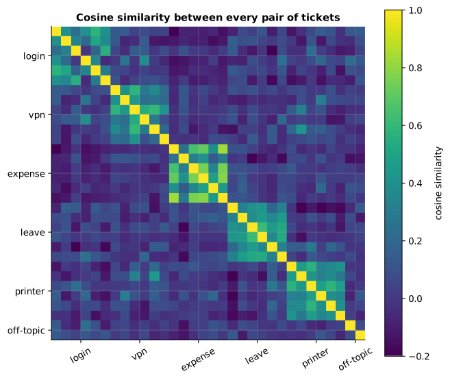
Reading it: rows and columns are the 32 tickets in the same order, grouped by kind, and brighter cells mean a higher cosine similarity. The five bright squares along the diagonal are the five kinds: tickets of one kind resemble each other and not the rest. The last two rows and columns (the off-topic tickets) are dark almost everywhere. Clustering is the job of finding those squares without knowing the order.
In code: ticket_embeddings returns the tickets' unit vectors and texts,
and ticket_kinds their true kinds, which the clustering never sees.
k-means: k meeting points
Everyday picture: a town wants k post boxes placed so that everyone's walk to their nearest box is as short as possible. Start with the boxes anywhere. Everyone walks to their nearest box; then each box moves to the middle of the people who chose it. Repeat until nobody switches box.
Tiny worked example: four points, (0, 0), (0, 1), (10, 0), (10, 1), and k = 2. However the boxes start, the two left points pick one box and the two right points the other. Each box moves to the middle of its pair: (0, 0.5) and (10, 0.5). Every point is now 0.5 away from its box, so the total squared walk is 4 × 0.5² = 1.0, and nothing changes on the next round.
flowchart LR
  I["Place k centres<br/>(k-means++: spread out)"] --> A["Assign: each point<br/>joins its nearest centre"]
  A --> M["Move: each centre goes to<br/>the mean of its points"]
  M --> C{Did any centre move?}
  C -->|yes| A
  C -->|no| D[Done: labels + centres]
Reading it: two steps alternate, assign and move, until the centres stop moving. Each step can only shrink the total squared distance (assigning to the nearest centre can't make anyone's walk longer; moving a centre to the mean of its points is the spot that minimizes their squared walks), so the loop always ends. The start matters: k-means++ picks each new starting centre far from the ones already chosen, which avoids two centres fighting over one crowd.
Level 3: the formula and its symbols
$$ J = \sum_{i=1}^{N} \lVert x_i - \mu_{c(i)} \rVert^2 $$
Symbols
| Symbol | Meaning here | Shape / range |
|---|---|---|
| J | the total squared distance, called inertia; k-means makes it small | ≥ 0 |
| N | number of points | 4 in the example; 30 tickets |
| i | which point | 1 to N |
| xᵢ | the i-th point (an embedding) | d numbers |
| c(i) | the cluster point i is assigned to | 1 to k |
| μ_c (mu) | the centroid of cluster c: the mean of its points | d numbers |
| ‖·‖² | squared Euclidean distance | ≥ 0 |
| Σ | add up over all points |
In words: add up, over every point, the squared distance from the point to the centre of its cluster.
On the example: four points each 0.5 from their centre: J = 4 × 0.25 = 1.0.
Level 3: in Python
In Python:
x = [(0, 0), (0, 1), (10, 0), (10, 1)]
# the two centroids
mu = [(0, 0.5), (10, 0.5)]
# c(i): the cluster each point joined
c = [0, 0, 1, 1]
# ‖x_i - μ_c(i)‖²
J = sum((x_i[0] - mu[c_i][0]) ** 2 + (x_i[1] - mu[c_i][1]) ** 2
        # Σ over every point
        for x_i, c_i in zip(x, c))
J  # → 1.0
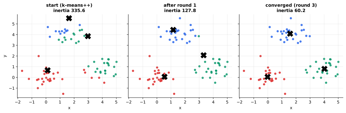
Reading it: three snapshots of k-means on 2-D points. Colours are the current assignments and black crosses are the centres. On the left, the k-means++ starting centres; in the middle, after the first assign-and-move round; on the right, the final state. The centres drift into the middle of their crowds and the total squared distance printed above each panel only goes down.
In code: kmeans alternates assign and move from k-means++ starts and
returns the labels, centres and inertia J of the best of several restarts;
kmeans_history records one run round by round, which is what this figure
draws.
Why it matters: k-means is fast and simple, and it's inside things you
use: IVF vector indexes cluster the corpus with it (primer.ml.embeddings.ann),
and topic discovery over tickets or documents often starts with it. Its
weaknesses are that you must choose k and that it assumes round, similar-sized
clusters.
Choosing k: the elbow and the silhouette
Everyday picture: at a party, you're in the right group if the people in your group are much closer to you than the people in the next group over.
Tiny worked example: the four points again, split into the two pairs. For (0, 0): its partner is a = 1 away; the other pair is 10 and √101 = 10.05 away, on average b = 10.025. Its score is (b − a) / b = 9.025 / 10.025 = 0.900, and by symmetry every point scores the same, so the silhouette is 0.900.
Level 3: the formula and its symbols
$$ s(i) = \frac{b(i) - a(i)}{\max\big(a(i), b(i)\big)} $$
Symbols
| Symbol | Meaning here | Range |
|---|---|---|
| s(i) | silhouette score of point i | −1 to 1 |
| a(i) | average distance from i to the other points in its own cluster | ≥ 0 |
| b(i) | average distance from i to the points of the nearest other cluster | ≥ 0 |
| max(a, b) | the larger of the two, to scale the score into −1 … 1 |
In words: how much farther the nearest other group is than your own, as a share of the larger distance. The silhouette of a clustering is the average over all points: near 1 is crisp, near 0 is overlapping, negative means points sit in the wrong cluster.
On the example: (10.025 − 1) / 10.025 = 0.900.
Level 3: in Python
In Python:
import math
# a(i): distance to its partner
a = math.dist((0, 0), (0, 1))
# b(i): the other pair, averaged
b = (math.dist((0, 0), (10, 0)) + math.dist((0, 0), (10, 1))) / 2
a, round(b, 3)  # → (1.0, 10.025)
# s(i)
round((b - a) / max(a, b), 3)  # → 0.9
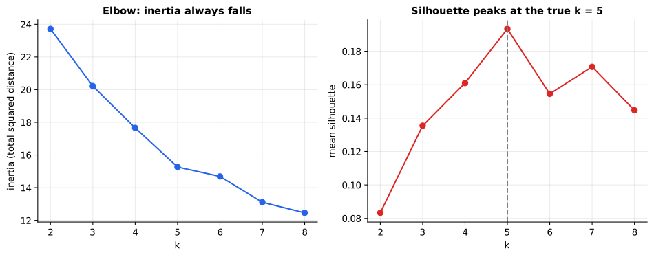
Reading it: both panels sweep k from 2 to 8 on the 30 tickets. On the left, inertia always falls as k grows (more boxes, shorter walks), so the lowest value is useless; you look for the elbow where it stops falling steeply. On the right, the silhouette has a clear peak at k = 5, the true number of ticket kinds. When the elbow is vague, the silhouette usually isn't.
In code: silhouette averages s(i) over every point, and
best_k_by_silhouette runs kmeans for each candidate k and keeps the one
with the highest silhouette.
Density clustering: DBSCAN and HDBSCAN
Everyday picture: a festival seen from a drone. A crowd is wherever people stand shoulder to shoulder; a loner by the fence belongs to no crowd. You don't decide in advance how many crowds there are.
Tiny worked example: points on a line at 0, 0.1, 0.2, 5.0, 5.1, 5.2 and 20, with reach ε = 0.15 and "a crowd needs at least 2". 0, 0.1 and 0.2 chain together (each within 0.15 of the next); so do 5.0, 5.1 and 5.2. 20 has nobody within 0.15. Result: two clusters and one noise point, labels 0 0 0 1 1 1 −1.
Level 3: the formula and its symbols
$$ N_\varepsilon(x) = {\, y : \text{dist}(x, y) \le \varepsilon \,}, \qquad x \text{ is a core point if } |N_\varepsilon(x)| \ge \text{minPts} $$
Symbols
| Symbol | Meaning here |
|---|---|
| x, y | points |
| dist | distance: Euclidean, or 1 − cosine for embeddings |
| ε (epsilon) | the reach: how close counts as "shoulder to shoulder" |
| N_ε(x) | the ε-neighbourhood: every point within reach of x (x included) |
| {… : …} | "the set of … such that …" |
| |·| | how many points are in the set |
| minPts | how many points within reach make x a core point |
In words: a point's neighbourhood is everything within reach; a point with enough neighbours is a core point; clusters grow outward from core points, and anything no core point can reach is noise.
On the example: N₀.₁₅(0.1) = {0, 0.1, 0.2}, 3 ≥ 2, so 0.1 is core; N₀.₁₅(20) = {20}, 1 < 2, so 20 is noise.
Level 3: in Python
In Python:
points = [0, 0.1, 0.2, 5.0, 5.1, 5.2, 20]
eps, minPts = 0.15, 2
# N_ε(x): every point within reach of x
def N(x):
    return [y for y in points if abs(x - y) <= eps]
# a core point
N(0.1), len(N(0.1)) >= minPts  # → ([0, 0.1, 0.2], True)
# nobody within reach: noise
N(20), len(N(20)) >= minPts  # → ([20], False)
flowchart TD
  P[Take an unvisited point] --> N{At least minPts<br/>within ε?}
  N -->|no| L[Leave it as noise for now]
  N -->|yes| S[Start a new cluster]
  S --> G[Add every neighbour;<br/>if a neighbour is also core,<br/>add its neighbours too]
  G --> G
  G --> P
  L --> P
Reading it: DBSCAN walks the points. A point with too few neighbours is left as noise (it can still be claimed later as the edge of someone else's crowd). A core point starts a cluster that floods outward through other core points, the self-loop on the "Add" box, until the crowd's edge is reached.
In code: dbscan finds the core points, floods each cluster outward
through them, and labels everything unreached −1 (noise).
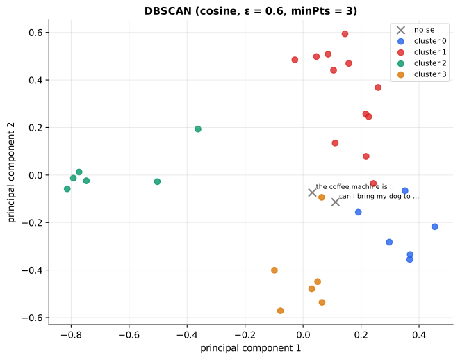
Reading it: the tickets drawn on the 2-D map from the next section, coloured by the clusters DBSCAN found (cosine distance, so ε = 0.6 means "cosine at least 0.4"; minPts = 3). Grey crosses are noise: exactly the two off-topic tickets, found without anyone telling DBSCAN how many clusters exist. Notice that VPN and printer tickets share a cluster: a chain of tickets that are each close to the next ("can't connect", "not working", "offline") bridges the two kinds.
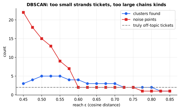
Reading it: the horizontal axis is the reach ε. The blue line counts clusters and the orange line counts noise points; the dashed line marks the two truly off-topic tickets. At the smallest reach (0.45) most tickets have too few neighbours: DBSCAN finds only three clusters and calls 22 of the 32 tickets noise. Between 0.5 and 0.55 it finds all five kinds, but still strands genuine tickets as noise (15, then 9). By 0.6 noise is down to just the off-topic pair, but kinds have already started chaining together (A is near B, B is near C, so A and C end up in one cluster): VPN and printer share a cluster, so only four are left. Keep widening and the chains keep growing, to three clusters, then two, until by 0.825 one cluster holds every kind and has swallowed an off-topic ticket as well, leaving a single noise point. No single ε gets everything right, and on real data you rarely know where the sweet spot is.
That's the problem HDBSCAN solves. It effectively runs DBSCAN at every reach at once, builds a tree of how crowds merge as the reach grows, and keeps the crowds that persist over the widest range of reaches. It handles clusters of different densities, needs no ε, and is the usual choice for exploring messy real text such as support tickets.
Seeing the map: PCA (and why UMAP and t-SNE mislead on distance)
Everyday picture: a shadow on a wall. A 3-D object casts a 2-D shadow; turn the object and the shadow changes. PCA (principal component analysis) turns the object so its shadow is as spread out as possible, keeping as much of the original variation as a flat picture can.
Tiny worked example: three points on a straight line, (1, 1), (2, 2), (3, 3). All their variation runs along the diagonal, so the first direction explains 100% of it and the second 0%. Along that direction the points sit √2 = 1.414 apart, exactly as in the original.
Level 3: the formula and its symbols
$$ \text{explained}_j = \frac{\sigma_j^2}{\sum_k \sigma_k^2} $$
Symbols
| Symbol | Meaning here | Range |
|---|---|---|
| j | which direction (principal component) | 1 to d |
| σⱼ (sigma) | the j-th singular value of the centred data, from the SVD (see primer.notation) |
≥ 0, largest first |
| σⱼ² | proportional to the variance (average squared spread) along direction j | ≥ 0 |
| Σₖ σₖ² | the total spread over all directions k | |
| explainedⱼ | the share of all the spread that direction j captures | 0 to 1 |
In words: the share of all the spread that direction j captures.
On the example: centred, the points are (−1, −1), (0, 0), (1, 1). Their singular values are 2 along the diagonal and 0 across it, so the shares are 2² / (2² + 0²) = 1 and 0 / 4 = 0.
Level 3: in Python
In Python:
import math
centred = [(-1, -1), (0, 0), (1, 1)]
# along the diagonal
u = [(1 / math.sqrt(2), 1 / math.sqrt(2)),
     # across it (the SVD finds these; here we know them)
     (1 / math.sqrt(2), -1 / math.sqrt(2))]
# spread along u_j
sigma = [math.sqrt(sum((x * u_j[0] + y * u_j[1]) ** 2 for x, y in centred))
         for u_j in u]
[round(sigma_j, 3) for sigma_j in sigma]  # → [2.0, 0.0]
[round(sigma_j ** 2 / sum(sigma_k ** 2 for sigma_k in sigma), 3) for sigma_j in sigma]  # → [1.0, 0.0]
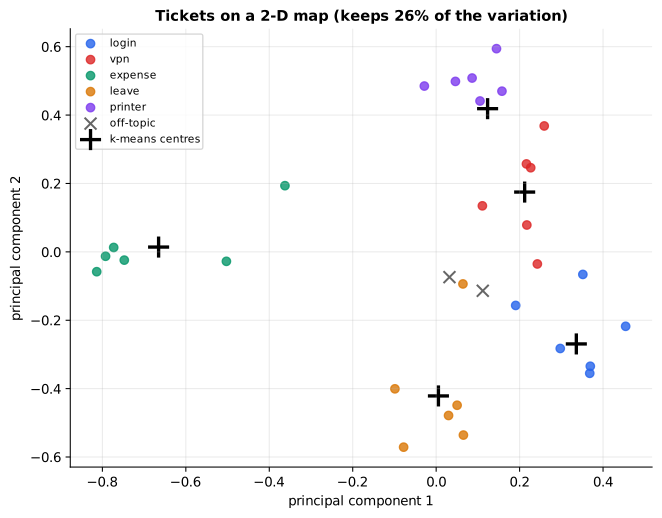
Reading it: the 128-dimensional ticket embeddings squashed to 2-D with PCA, coloured by their true kind; black crosses are the k-means centres, projected the same way, and the grey ✕ markers are the off-topic tickets. Kinds form separate patches and the centres sit inside them. The title says what share of the variation the two axes keep: the rest is invisible here, so tickets that look close on this map can be far apart in the real space.
In code: pca centres the data, projects it onto the top n directions
from the SVD, and returns each direction's explained share.
UMAP and t-SNE draw prettier maps by a different rule: keep each point's neighbours next to it, and let distances elsewhere stretch. Like a subway map, they're great for "what's near what" and misleading for "how far" or "how big": gaps between clusters and cluster sizes in those plots don't reflect the real space. Use them for intuition, never for measurement.
Everyday uses
flowchart LR
  T[New text] --> E[Embed]
  E --> D{Nearly identical to<br/>something stored?}
  D -->|yes| DUP[Near-duplicate:<br/>merge or skip]
  E --> R{Closest route centroid<br/>above threshold?}
  R -->|yes| ROUTE[Send to that team/tool]
  R -->|no| HUMAN[Fallback: human or<br/>general assistant]
  E --> A{Far from every<br/>cluster centre?}
  A -->|yes| ANOM[Flag as anomaly]
  E --> C{Cached question, same context,<br/>not expired, above threshold?}
  C -->|yes| HIT[Return cached answer]
Reading it: one embedding feeds four independent checks, each a comparison with things already known. All four have the same shape: a distance and a threshold. What differs is what's being compared against (stored documents, route examples, cluster centres, cached questions) and what happens on a hit.
Near-duplicates. Photocopies with a sticky note on them: nearly
identical vectors. "password reset link expired" and "The password reset
link has expired!" score cosine 1.0 here; flag pairs above a threshold
calibrated on labeled pairs (primer.ml.embeddings.similarity).
In code: near_duplicates embeds a list of texts and returns every pair
whose cosine reaches the threshold.
Routing. A receptionist listening to a request and pointing to the right desk. Each route (a team, a tool, an agent) is represented by the centroid of a few example requests; a new request goes to the closest centroid, or to a fallback when nothing is close:
Level 3: the formula and its symbols
$$ \text{route}(q) = \begin{cases} \arg\max_r \cos(q, \mu_r) & \text{if } \max_r \cos(q, \mu_r) \ge \theta \ \text{fallback} & \text{otherwise} \end{cases} $$
Symbols
| Symbol | Meaning here | Range |
|---|---|---|
| q | the incoming request's embedding | unit vector |
| r | a route: a team, tool or agent | it_helpdesk, finance, hr |
| μᵣ (mu) | route r's centroid: the mean of its example requests, rescaled to length 1 | unit vector |
| cos(q, μᵣ) | cosine similarity of the request with that route | −1 to 1 |
| arg maxᵣ | the route that gives the largest value | |
| θ (theta) | the confidence threshold | 0.3 here |
In words: send the request to the route it's most similar to, unless even the best match is weak, in which case hand it off.
On the example: "my vpn tunnel drops when I work remote" scores highest against the IT helpdesk; "what is the capital of france" is near 0 against every route, below θ = 0.3, so it goes to the fallback.
With the numbers: a toy version with three routes in four dimensions: μ_it = (1, 0, 0, 0), μ_finance = (0, 1, 0, 0), μ_hr = (0, 0, 1, 0). The request q = (0.8, 0.6, 0, 0) has cosines 0.8, 0.6 and 0.0 with them; the best, 0.8, clears θ = 0.3, so it goes to it_helpdesk. The request q = (0.1, 0.2, 0, 1) points mostly where no route lies: its cosines are about 0.1, 0.2 and 0.0, all below θ, so it goes to the fallback.
Level 3: in Python
In Python:
import math
def cos(a, b):
    dot = sum(a_k * b_k for a_k, b_k in zip(a, b))
    return dot / (math.sqrt(sum(a_k ** 2 for a_k in a)) * math.sqrt(sum(b_k ** 2 for b_k in b)))
mu = {"it_helpdesk": (1, 0, 0, 0), "finance": (0, 1, 0, 0), "hr": (0, 0, 1, 0)}
theta = 0.3
def route(q):
    scores = {r: cos(q, mu_r) for r, mu_r in mu.items()}
    # arg max_r cos(q, μ_r)
    best = max(scores, key=scores.get)
    return best if scores[best] >= theta else "fallback"
[round(cos((0.8, 0.6, 0, 0), mu_r), 2) for mu_r in mu.values()], route((0.8, 0.6, 0, 0))  # → ([0.8, 0.6, 0.0], 'it_helpdesk')
[round(cos((0.1, 0.2, 0, 1), mu_r), 2) for mu_r in mu.values()], route((0.1, 0.2, 0, 1))  # → ([0.1, 0.2, 0.0], 'fallback')
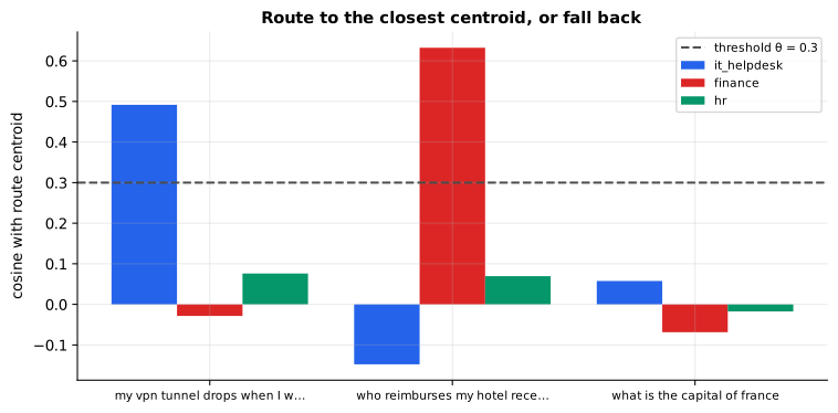
Reading it: each group of bars is one incoming request; each bar is its cosine with one route's centroid; the dashed line is the threshold θ. The VPN complaint clears the line only for IT, the receipt question only for finance, and the off-topic question clears nothing, so it goes to a human. The fallback is the important part: a router without one sends every unanswerable question somewhere.
In code: Router holds one unit-length centroid per route;
Router.scores gives a request's cosine with each, and Router.route
applies θ and the fallback. support_router builds the lesson's three
routes.
Anomaly detection. A stranger at a party is far from every group. Score each item by its distance to the nearest cluster centre; the largest scores are the unusual items. Here the coffee machine and the dog come out on top.
In code: anomaly_scores returns each point's distance to its nearest
cluster centre.
Semantic caching. An FAQ desk that remembers answers. If a new question means the same as one already answered, return the stored answer and skip the model call, saving cost and latency. Three guards keep it safe:
- A strict, calibrated threshold. "How do I reset my VPN?" is only about 0.46 similar to "How do I reset my password?" here: related, but a different question.
- A context key. "What is my PTO balance?" means something different for Alice and Bob. Answers are only reused within the same user, tenant and permission scope.
- Expiry. A time-to-live, so answers age out when the facts change.
flowchart LR
  Q[Question + context] --> F[Keep entries with the<br/>same context, not expired]
  F --> S[Most similar entry]
  S --> T{cosine ≥ threshold?}
  T -->|yes| H[Hit: return stored answer]
  T -->|no| M[Miss: call the model,<br/>store the new answer]
Reading it: the filter comes before the similarity search, not after: an answer from another user's context is never even a candidate, so no threshold setting can leak it. Only then does similarity decide.
In code: SemanticCache.put stores a question, its answer and its
context; SemanticCache.lookup filters by context and expiry, then finds the
most similar entry, and SemanticCache.get returns its answer only above the
threshold.
In 20 seconds
- k-means alternates "assign to nearest centre" and "move centre to the mean"; you choose k, using the silhouette or the elbow.
- DBSCAN/HDBSCAN find crowds by density, choose the number of clusters themselves, and mark loners as noise; better for messy text.
- PCA gives an honest but lossy 2-D shadow; UMAP/t-SNE keep neighbours but distort distances and sizes.
- Near-duplicates, routing, anomaly detection and semantic caching are all "embed, compare, threshold".
- Semantic caches need a strict threshold, a context key and an expiry.
Self-test questions
Q: How does k-means work, and what are its limitations? Alternate assigning each point to its nearest centre and moving each centre to the mean of its points until nothing changes. You must choose k, results depend on the start (k-means++ helps), and it assumes round, similar-sized clusters.
Q: When would you choose HDBSCAN over k-means for text embeddings? When you don't know how many groups exist, clusters have different shapes and densities, and some items belong nowhere (support tickets, logs). It finds the number of clusters itself and labels outliers as noise.
Q: Why can't you trust distances in a UMAP or t-SNE plot? They preserve local neighbourhoods and deliberately distort everything else, so gaps between clusters and cluster sizes don't reflect the real space.
Q: How would you route requests to the right agent or tool with embeddings? Represent each route by the centroid of example requests, send each new request to the most similar centroid, and fall back to a human or general assistant when the best similarity is below a calibrated threshold.
Q: What can go wrong with a semantic cache? A loose threshold returns the answer to a different question; missing context keys leak one user's or tenant's answer to another; missing expiry serves stale facts. Filter by context first, then match strictly, and expire entries.
The papers behind this lesson
- Arthur and Vassilvitskii, k-means++: The Advantages of Careful Seeding (2007): https://dl.acm.org/doi/10.5555/1283383.1283494. Showed that spreading out the starting centres makes k-means provably close to optimal and much faster to converge.
- Ester, Kriegel, Sander and Xu, A Density-Based Algorithm for Discovering Clusters (DBSCAN, 1996): https://dl.acm.org/doi/10.5555/3001460.3001507. Defined clusters as dense regions reachable through core points, with everything else as noise.
- Campello, Moulavi and Sander, Density-Based Clustering Based on Hierarchical Density Estimates (HDBSCAN, 2013): https://doi.org/10.1007/978-3-642-37456-2_14. Removed DBSCAN's single reach parameter by building a hierarchy over all reaches and keeping the most persistent clusters.
- McInnes, Healy and Melville, UMAP (2018): https://arxiv.org/abs/1802.03426. A fast neighbour-preserving projection now standard for visualizing embeddings.
Further reading
- scikit-learn user guide, clustering: https://scikit-learn.org/stable/modules/clustering.html
- hdbscan documentation, How HDBSCAN Works: https://hdbscan.readthedocs.io/en/latest/how_hdbscan_works.html
- UMAP documentation: https://umap-learn.readthedocs.io/
- Wattenberg, Viégas and Johnson, How to Use t-SNE Effectively (Distill): https://distill.pub/2016/misread-tsne/
1r""" 2# Clustering and everyday uses of embeddings: grouping, mapping, routing, caching 3 4Run: `python -m primer.ml.embeddings.clustering` 5 6New to vectors, distances or Σ? `primer.notation` builds them from zero. 7 8## Level 1: The practitioner's guide 9 10**In one sentence.** Clustering groups texts by meaning without being told 11what the groups are, and the move behind it, one distance and one threshold, 12also powers four everyday jobs: spotting near-duplicates, routing requests, 13flagging anomalies and caching answers. 14 15**When you need it.** You need clustering when you have a pile of unlabeled 16text (support tickets, feedback, logs, documents) and want to know what 17kinds of things are in it before anyone has named the kinds. You need the 18everyday uses whenever the question is "have I seen something like this 19before?": the same ticket filed twice, a request that belongs to another 20team, an entry that looks like nothing else, a question already answered an 21hour ago. You don't need clustering when the categories are already known 22and labeled: that is classification, and a centroid per class or a trained 23model does it directly. The tell: someone is reading tickets one by one to 24find out what people are asking about, or a model is being called again for 25a question it has already answered. 26 27**Your options.** From the simplest to the most flexible: 28 29| Option | What it does | What it gives you | What it costs | Where it lives | 30|---|---|---|---|---| 31| One distance and a threshold | Embeds the new item and compares it with what is already stored | Near-duplicate detection, routing, anomaly scores and a semantic cache, with no clustering at all | A threshold to calibrate on labeled pairs, plus the guards below | Your code over any embedding model; semantic-router, GPTCache | 32| k-means | Alternates "assign each point to its nearest centre" and "move each centre to the mean of its points" | k crisp groups with a centre each; fast, and scikit-learn lists it for very large collections | You choose k, and it assumes round, similar-sized clusters | scikit-learn, FAISS (it is how IVF indexes cluster a corpus) | 33| DBSCAN | Grows clusters through points with enough neighbours within a reach ε, leaving the rest as noise | The number of clusters found for you, and loners marked as noise | A reach no single value gets right; kinds chain together as it widens | scikit-learn | 34| HDBSCAN | Runs DBSCAN at every reach at once and keeps the clusters that persist longest | Clusters of different densities, no ε to set, noise labelled | A minimum cluster size to pick; listed for large rather than very large collections | scikit-learn, the hdbscan library, BERTopic | 35| Agglomerative (hierarchical) | Merges the closest pair of groups again and again into a tree | Many clusters, a cut at any level, any distance | You still choose where to cut the tree | scikit-learn | 36 37**How to choose.** Start from whether you know how many groups there are 38and whether every item belongs somewhere. 39 40- You know the number of groups, or want a fixed number of buckets (topics 41 for a dashboard, cells for a vector index): k-means, seeded with 42 k-means++. Pick k by the silhouette, not the inertia: inertia falls at 43 every k, while the silhouette peaks at the true number (k = 5 for this 44 lesson's five ticket kinds). 45- You don't know how many groups exist, some items belong nowhere, and the 46 groups differ in shape and density (real tickets, logs): HDBSCAN. Plain 47 DBSCAN is the same idea with one reach you have to guess, and on this 48 lesson's tickets no reach gets everything right. 49- You want a picture: PCA for an honest but lossy shadow (its title tells 50 you what share of the variation you are seeing); UMAP or t-SNE for a 51 prettier map of what is near what, never for measuring distances or 52 cluster sizes. 53- You want an action per item rather than groups: the threshold pattern. 54 Flag near-duplicate pairs above a calibrated cosine, send a request to the 55 route whose centroid clears the threshold, score an anomaly by its 56 distance to the nearest centre, return a cached answer only above a strict 57 threshold. 58- Whatever you pick, calibrate every threshold on labeled pairs from your 59 own data, check the clusters against a sample you have read, and keep the 60 fallback: a router without one sends every unanswerable question 61 somewhere. 62 63**What it costs.** Everything here runs on embeddings you already have, so 64the model cost is one embedding per item. k-means is the cheap one: a few 65rounds of assign-and-move, restarted a few times, with the total squared 66distance only ever falling. DBSCAN's naive form needs every pairwise 67distance, which scikit-learn notes costs n² floats of memory when its tree 68structures can't be used; HDBSCAN does more work than k-means for its freedom 69from ε. The everyday uses cost one comparison against what is stored, and a 70semantic cache pays for itself by skipping a model call on every hit, at the 71risk of a wrong hit: GPTCache's documentation says plainly that a semantic 72cache produces false positives on hits and false negatives on misses. The 73real expense is labeling: a few dozen labeled pairs to calibrate a 74threshold, and a sample of items read by a person to check that the 75clusters mean what you think. 76 77**What breaks.** 78 79- **The wrong k.** Inertia keeps falling as k grows, so the lowest value is 80 useless. Use the silhouette, or the elbow where inertia stops falling 81 steeply. 82- **Chaining.** Widen DBSCAN's reach until real tickets stop being noise and 83 kinds merge through chains of near neighbours: at ε = 0.6 here the noise 84 is exactly the two off-topic tickets, but VPN and printer tickets share a 85 cluster. HDBSCAN keeps the clusters that persist across reaches instead. 86- **Loners forced into a group.** k-means gives every point a cluster, 87 including the coffee-machine and dog tickets that belong to none. Use a 88 density method, or score anomalies by distance to the nearest centre. 89- **Distances read off a UMAP or t-SNE plot.** Gaps between clusters and 90 cluster sizes there don't reflect the real space. Use the map for 91 intuition, measure in the original space. 92- **A cache that answers a different question.** "How do I reset my VPN?" 93 is about 0.46 similar to "How do I reset my password?" here: related, and 94 wrong. Keep the threshold strict and calibrated. 95- **A cache that leaks across users.** "What is my PTO balance?" means 96 something different for each person. Filter by user, tenant and 97 permission scope before the similarity search, so no threshold setting 98 can leak an answer. 99- **Stale hits.** Give every entry a time-to-live so answers age out when 100 the facts change. 101- **A router without a fallback.** Below the threshold, hand the request to 102 a person or a general assistant rather than the least-bad route. 103 104**In the wild.** scikit-learn ships k-means, DBSCAN, HDBSCAN and 105agglomerative clustering with a guide to which fits which data (k-means for 106even cluster sizes and flat geometry, DBSCAN and HDBSCAN for uneven sizes 107and outlier removal, HDBSCAN when densities vary); the hdbscan library and 108umap-learn are the reference implementations of their papers. FAISS runs 109k-means to build the cells of an IVF index. BERTopic discovers topics by 110chaining sentence-transformers embeddings, UMAP, HDBSCAN and a class-based 111TF-IDF. semantic-router defines each route by example utterances, embeds 112them, and returns no route at all when nothing matches, with thresholds you 113can train. GPTCache embeds each query, searches a vector store and lets a 114similarity evaluator decide the hit. The papers behind this lesson 115(k-means++, DBSCAN, HDBSCAN and UMAP) are listed at the end, and Distill's 116*How to Use t-SNE Effectively* shows the misreadings the map warning above 117is about. 118 119**Go deeper.** Level 2 builds k-means, the silhouette, DBSCAN, PCA and all 120four everyday uses by hand, first on four points you can check with a 121pencil and then on thirty support tickets, with every formula decoded and 122every figure explained. If you only needed to choose a method and set its 123thresholds, you are done. 124 125## Level 2: How it works, from scratch 126 127Level 2 builds each of those methods from nothing, starting with a sack of 128mail. 129 130**The everyday picture.** Tip a sack of unlabeled mail onto a table and sort it into piles by what 131each letter is about. Nobody gave you the pile names; you notice that some 132letters are about passwords and others about holidays, and similar letters 133end up together. That's **clustering**: finding groups in data without being 134told what the groups are. 135 136Embeddings make it possible for text. Every ticket, email or document gets 137coordinates on a map of meaning (`primer.ml.embeddings.similarity`), so 138"similar" becomes "close", and sorting mail becomes finding crowds of nearby 139points. The same closeness also powers four everyday jobs: spotting 140**near-duplicates**, **routing** requests to the right team, flagging 141**anomalies**, and **caching** answers to questions already asked. 142 143This lesson uses 30 short IT, HR and finance support tickets (five kinds, six 144of each) and two off-topic ones, embedded with the repo's toy embedder 145(`primer.common.embedder`). 146 147 148 149**Reading it:** rows and columns are the 32 tickets in the same order, grouped 150by kind, and brighter cells mean a higher cosine similarity. The five bright 151squares along the diagonal are the five kinds: tickets of one kind resemble 152each other and not the rest. The last two rows and columns (the off-topic 153tickets) are dark almost everywhere. Clustering is the job of finding those 154squares *without* knowing the order. 155 156**In code:** `ticket_embeddings` returns the tickets' unit vectors and texts, 157and `ticket_kinds` their true kinds, which the clustering never sees. 158 159## k-means: k meeting points 160 161**Everyday picture:** a town wants k post boxes placed so that everyone's 162walk to their nearest box is as short as possible. Start with the boxes 163anywhere. Everyone walks to their nearest box; then each box moves to the 164middle of the people who chose it. Repeat until nobody switches box. 165 166**Tiny worked example:** four points, (0, 0), (0, 1), (10, 0), (10, 1), and 167k = 2. However the boxes start, the two left points pick one box and the two 168right points the other. Each box moves to the middle of its pair: (0, 0.5) and 169(10, 0.5). Every point is now 0.5 away from its box, so the total squared 170walk is 4 × 0.5² = **1.0**, and nothing changes on the next round. 171 172```mermaid 173flowchart LR 174 I["Place k centres<br/>(k-means++: spread out)"] --> A["Assign: each point<br/>joins its nearest centre"] 175 A --> M["Move: each centre goes to<br/>the mean of its points"] 176 M --> C{Did any centre move?} 177 C -->|yes| A 178 C -->|no| D[Done: labels + centres] 179``` 180 181**Reading it:** two steps alternate, assign and move, until the centres stop 182moving. Each step can only shrink the total squared distance (assigning to 183the nearest centre can't make anyone's walk longer; moving a centre to the 184mean of its points is the spot that minimizes their squared walks), so the 185loop always ends. The start matters: **k-means++** picks each new starting 186centre far from the ones already chosen, which avoids two centres fighting 187over one crowd. 188 189$$ 190J = \sum_{i=1}^{N} \lVert x_i - \mu_{c(i)} \rVert^2 191$$ 192 193**Symbols** 194 195| Symbol | Meaning here | Shape / range | 196|---|---|---| 197| J | the total squared distance, called **inertia**; k-means makes it small | ≥ 0 | 198| N | number of points | 4 in the example; 30 tickets | 199| i | which point | 1 to N | 200| xᵢ | the i-th point (an embedding) | d numbers | 201| c(i) | the cluster point i is assigned to | 1 to k | 202| μ_c (mu) | the **centroid** of cluster c: the mean of its points | d numbers | 203| ‖·‖² | squared Euclidean distance | ≥ 0 | 204| Σ | add up over all points | | 205 206**In words:** add up, over every point, the squared distance from the point 207to the centre of its cluster. 208 209**On the example:** four points each 0.5 from their centre: J = 4 × 0.25 = 1.0. 210 211**In Python:** 212 213```python 214x = [(0, 0), (0, 1), (10, 0), (10, 1)] 215# the two centroids 216mu = [(0, 0.5), (10, 0.5)] 217# c(i): the cluster each point joined 218c = [0, 0, 1, 1] 219# ‖x_i - μ_c(i)‖² 220J = sum((x_i[0] - mu[c_i][0]) ** 2 + (x_i[1] - mu[c_i][1]) ** 2 221 # Σ over every point 222 for x_i, c_i in zip(x, c)) 223J # → 1.0 224``` 225 226 227 228**Reading it:** three snapshots of k-means on 2-D points. Colours are the 229current assignments and black crosses are the centres. On the left, the 230k-means++ starting centres; in the middle, after the first assign-and-move 231round; on the right, the final state. The centres drift into the middle of 232their crowds and the total squared distance printed above each panel only 233goes down. 234 235**In code:** `kmeans` alternates assign and move from k-means++ starts and 236returns the labels, centres and inertia J of the best of several restarts; 237`kmeans_history` records one run round by round, which is what this figure 238draws. 239 240**Why it matters:** k-means is fast and simple, and it's inside things you 241use: IVF vector indexes cluster the corpus with it (`primer.ml.embeddings.ann`), 242and topic discovery over tickets or documents often starts with it. Its 243weaknesses are that you must choose k and that it assumes round, similar-sized 244clusters. 245 246## Choosing k: the elbow and the silhouette 247 248**Everyday picture:** at a party, you're in the right group if the people in 249your group are much closer to you than the people in the next group over. 250 251**Tiny worked example:** the four points again, split into the two pairs. 252For (0, 0): its partner is a = **1** away; the other pair is 10 and √101 = 10.05 253away, on average b = **10.025**. Its score is (b − a) / b = 9.025 / 10.025 = **0.900**, 254and by symmetry every point scores the same, so the silhouette is 0.900. 255 256$$ 257s(i) = \frac{b(i) - a(i)}{\max\big(a(i), b(i)\big)} 258$$ 259 260**Symbols** 261 262| Symbol | Meaning here | Range | 263|---|---|---| 264| s(i) | silhouette score of point i | −1 to 1 | 265| a(i) | average distance from i to the other points in its own cluster | ≥ 0 | 266| b(i) | average distance from i to the points of the *nearest other* cluster | ≥ 0 | 267| max(a, b) | the larger of the two, to scale the score into −1 … 1 | | 268 269**In words:** how much farther the nearest other group is than your own, 270as a share of the larger distance. The silhouette of a clustering is the 271average over all points: near 1 is crisp, near 0 is overlapping, negative 272means points sit in the wrong cluster. 273 274**On the example:** (10.025 − 1) / 10.025 = 0.900. 275 276**In Python:** 277 278```python 279import math 280# a(i): distance to its partner 281a = math.dist((0, 0), (0, 1)) 282# b(i): the other pair, averaged 283b = (math.dist((0, 0), (10, 0)) + math.dist((0, 0), (10, 1))) / 2 284a, round(b, 3) # → (1.0, 10.025) 285# s(i) 286round((b - a) / max(a, b), 3) # → 0.9 287``` 288 289 290 291**Reading it:** both panels sweep k from 2 to 8 on the 30 tickets. On the 292left, inertia always falls as k grows (more boxes, shorter walks), so the 293lowest value is useless; you look for the **elbow** where it stops falling 294steeply. On the right, the silhouette has a clear peak at k = 5, the true 295number of ticket kinds. When the elbow is vague, the silhouette usually 296isn't. 297 298**In code:** `silhouette` averages s(i) over every point, and 299`best_k_by_silhouette` runs `kmeans` for each candidate k and keeps the one 300with the highest silhouette. 301 302## Density clustering: DBSCAN and HDBSCAN 303 304**Everyday picture:** a festival seen from a drone. A crowd is wherever 305people stand shoulder to shoulder; a loner by the fence belongs to no crowd. 306You don't decide in advance how many crowds there are. 307 308**Tiny worked example:** points on a line at 0, 0.1, 0.2, 5.0, 5.1, 5.2 and 20, 309with reach ε = 0.15 and "a crowd needs at least 2". 0, 0.1 and 0.2 chain 310together (each within 0.15 of the next); so do 5.0, 5.1 and 5.2. 20 has nobody 311within 0.15. Result: two clusters and one noise point, labels 312**0 0 0 1 1 1 −1**. 313 314$$ 315N_\varepsilon(x) = \{\, y : \text{dist}(x, y) \le \varepsilon \,\}, \qquad 316x \text{ is a core point if } |N_\varepsilon(x)| \ge \text{minPts} 317$$ 318 319**Symbols** 320 321| Symbol | Meaning here | 322|---|---| 323| x, y | points | 324| dist | distance: Euclidean, or 1 − cosine for embeddings | 325| ε (epsilon) | the reach: how close counts as "shoulder to shoulder" | 326| N_ε(x) | the ε-neighbourhood: every point within reach of x (x included) | 327| {… : …} | "the set of … such that …" | 328| \|·\| | how many points are in the set | 329| minPts | how many points within reach make x a **core** point | 330 331**In words:** a point's neighbourhood is everything within reach; a point 332with enough neighbours is a core point; clusters grow outward from core 333points, and anything no core point can reach is noise. 334 335**On the example:** N₀.₁₅(0.1) = {0, 0.1, 0.2}, 3 ≥ 2, so 0.1 is core; 336N₀.₁₅(20) = {20}, 1 < 2, so 20 is noise. 337 338**In Python:** 339 340```python 341points = [0, 0.1, 0.2, 5.0, 5.1, 5.2, 20] 342eps, minPts = 0.15, 2 343# N_ε(x): every point within reach of x 344def N(x): 345 return [y for y in points if abs(x - y) <= eps] 346# a core point 347N(0.1), len(N(0.1)) >= minPts # → ([0, 0.1, 0.2], True) 348# nobody within reach: noise 349N(20), len(N(20)) >= minPts # → ([20], False) 350``` 351 352```mermaid 353flowchart TD 354 P[Take an unvisited point] --> N{At least minPts<br/>within ε?} 355 N -->|no| L[Leave it as noise for now] 356 N -->|yes| S[Start a new cluster] 357 S --> G[Add every neighbour;<br/>if a neighbour is also core,<br/>add its neighbours too] 358 G --> G 359 G --> P 360 L --> P 361``` 362 363**Reading it:** DBSCAN walks the points. A point with too few neighbours is 364left as noise (it can still be claimed later as the edge of someone else's 365crowd). A core point starts a cluster that floods outward through other core 366points, the self-loop on the "Add" box, until the crowd's edge is reached. 367 368**In code:** `dbscan` finds the core points, floods each cluster outward 369through them, and labels everything unreached −1 (noise). 370 371 372 373**Reading it:** the tickets drawn on the 2-D map from the next section, 374coloured by the clusters DBSCAN found (cosine distance, so ε = 0.6 means 375"cosine at least 0.4"; minPts = 3). Grey crosses are noise: exactly the two 376off-topic tickets, found without anyone telling DBSCAN how many clusters 377exist. Notice that VPN and printer tickets share a cluster: a chain of 378tickets that are each close to the next ("can't connect", "not working", 379"offline") bridges the two kinds. 380 381 382 383**Reading it:** the horizontal axis is the reach ε. The blue line counts 384clusters and the orange line counts noise points; the dashed line marks the 385two truly off-topic tickets. At the smallest reach (0.45) most tickets have 386too few neighbours: DBSCAN finds only three clusters and calls 22 of the 32 387tickets noise. Between 0.5 and 0.55 it finds all five kinds, but still 388strands genuine tickets as noise (15, then 9). By 0.6 noise is down to just 389the off-topic pair, but kinds have already started **chaining** together (A 390is near B, B is near C, so A and C end up in one cluster): VPN and printer 391share a cluster, so only four are left. Keep widening and the chains keep 392growing, to three clusters, then two, until by 0.825 one cluster holds every 393kind and has swallowed an off-topic ticket as well, leaving a single noise 394point. No single ε gets everything right, and on real data you rarely know 395where the sweet spot is. 396 397That's the problem **HDBSCAN** solves. It effectively runs DBSCAN at every 398reach at once, builds a tree of how crowds merge as the reach grows, and keeps 399the crowds that persist over the widest range of reaches. It handles clusters 400of different densities, needs no ε, and is the usual choice for exploring 401messy real text such as support tickets. 402 403## Seeing the map: PCA (and why UMAP and t-SNE mislead on distance) 404 405**Everyday picture:** a shadow on a wall. A 3-D object casts a 2-D shadow; 406turn the object and the shadow changes. **PCA** (principal component 407analysis) turns the object so its shadow is as spread out as possible, 408keeping as much of the original variation as a flat picture can. 409 410**Tiny worked example:** three points on a straight line, (1, 1), (2, 2), 411(3, 3). All their variation runs along the diagonal, so the first direction 412explains **100%** of it and the second **0%**. Along that direction the points 413sit √2 = **1.414** apart, exactly as in the original. 414 415$$ 416\text{explained}_j = \frac{\sigma_j^2}{\sum_k \sigma_k^2} 417$$ 418 419**Symbols** 420 421| Symbol | Meaning here | Range | 422|---|---|---| 423| j | which direction (principal component) | 1 to d | 424| σⱼ (sigma) | the j-th singular value of the centred data, from the SVD (see `primer.notation`) | ≥ 0, largest first | 425| σⱼ² | proportional to the **variance** (average squared spread) along direction j | ≥ 0 | 426| Σₖ σₖ² | the total spread over all directions k | | 427| explainedⱼ | the share of all the spread that direction j captures | 0 to 1 | 428 429**In words:** the share of all the spread that direction j captures. 430 431**On the example:** centred, the points are (−1, −1), (0, 0), (1, 1). Their 432singular values are 2 along the diagonal and 0 across it, so the shares are 4332² / (2² + 0²) = 1 and 0 / 4 = 0. 434 435**In Python:** 436 437```python 438import math 439centred = [(-1, -1), (0, 0), (1, 1)] 440# along the diagonal 441u = [(1 / math.sqrt(2), 1 / math.sqrt(2)), 442 # across it (the SVD finds these; here we know them) 443 (1 / math.sqrt(2), -1 / math.sqrt(2))] 444# spread along u_j 445sigma = [math.sqrt(sum((x * u_j[0] + y * u_j[1]) ** 2 for x, y in centred)) 446 for u_j in u] 447[round(sigma_j, 3) for sigma_j in sigma] # → [2.0, 0.0] 448[round(sigma_j ** 2 / sum(sigma_k ** 2 for sigma_k in sigma), 3) for sigma_j in sigma] # → [1.0, 0.0] 449``` 450 451 452 453**Reading it:** the 128-dimensional ticket embeddings squashed to 2-D with 454PCA, coloured by their true kind; black crosses are the k-means centres, 455projected the same way, and the grey ✕ markers are the off-topic tickets. 456Kinds form separate patches and the centres sit inside them. The title says 457what share of the variation the two axes keep: the rest is invisible here, 458so tickets that look close on this map can be far apart in the real space. 459 460**In code:** `pca` centres the data, projects it onto the top n directions 461from the SVD, and returns each direction's explained share. 462 463UMAP and t-SNE draw prettier maps by a different rule: keep each point's 464*neighbours* next to it, and let distances elsewhere stretch. Like a subway 465map, they're great for "what's near what" and misleading for "how far" or 466"how big": gaps between clusters and cluster sizes in those plots don't 467reflect the real space. Use them for intuition, never for measurement. 468 469## Everyday uses 470 471```mermaid 472flowchart LR 473 T[New text] --> E[Embed] 474 E --> D{Nearly identical to<br/>something stored?} 475 D -->|yes| DUP[Near-duplicate:<br/>merge or skip] 476 E --> R{Closest route centroid<br/>above threshold?} 477 R -->|yes| ROUTE[Send to that team/tool] 478 R -->|no| HUMAN[Fallback: human or<br/>general assistant] 479 E --> A{Far from every<br/>cluster centre?} 480 A -->|yes| ANOM[Flag as anomaly] 481 E --> C{Cached question, same context,<br/>not expired, above threshold?} 482 C -->|yes| HIT[Return cached answer] 483``` 484 485**Reading it:** one embedding feeds four independent checks, each a 486comparison with things already known. All four have the same shape: a 487distance and a threshold. What differs is what's being compared against 488(stored documents, route examples, cluster centres, cached questions) and 489what happens on a hit. 490 491**Near-duplicates.** Photocopies with a sticky note on them: nearly 492identical vectors. "password reset link expired" and "The password reset 493link has expired!" score cosine 1.0 here; flag pairs above a threshold 494calibrated on labeled pairs (`primer.ml.embeddings.similarity`). 495 496**In code:** `near_duplicates` embeds a list of texts and returns every pair 497whose cosine reaches the threshold. 498 499**Routing.** A receptionist listening to a request and pointing to the right 500desk. Each route (a team, a tool, an agent) is represented by the centroid 501of a few example requests; a new request goes to the closest centroid, or to 502a fallback when nothing is close: 503 504$$ 505\text{route}(q) = 506\begin{cases} 507\arg\max_r \cos(q, \mu_r) & \text{if } \max_r \cos(q, \mu_r) \ge \theta \\ 508\text{fallback} & \text{otherwise} 509\end{cases} 510$$ 511 512**Symbols** 513 514| Symbol | Meaning here | Range | 515|---|---|---| 516| q | the incoming request's embedding | unit vector | 517| r | a route: a team, tool or agent | it_helpdesk, finance, hr | 518| μᵣ (mu) | route r's centroid: the mean of its example requests, rescaled to length 1 | unit vector | 519| cos(q, μᵣ) | cosine similarity of the request with that route | −1 to 1 | 520| arg maxᵣ | the route that gives the largest value | | 521| θ (theta) | the confidence threshold | 0.3 here | 522 523**In words:** send the request to the route it's most similar to, unless even 524the best match is weak, in which case hand it off. 525 526**On the example:** "my vpn tunnel drops when I work remote" scores highest 527against the IT helpdesk; "what is the capital of france" is near 0 against 528every route, below θ = 0.3, so it goes to the fallback. 529 530**With the numbers:** a toy version with three routes in four dimensions: 531μ_it = (1, 0, 0, 0), μ_finance = (0, 1, 0, 0), μ_hr = (0, 0, 1, 0). The request 532q = (0.8, 0.6, 0, 0) has cosines 0.8, 0.6 and 0.0 with them; the best, 0.8, 533clears θ = 0.3, so it goes to it_helpdesk. The request q = (0.1, 0.2, 0, 1) 534points mostly where no route lies: its cosines are about 0.1, 0.2 and 0.0, 535all below θ, so it goes to the fallback. 536 537**In Python:** 538 539```python 540import math 541def cos(a, b): 542 dot = sum(a_k * b_k for a_k, b_k in zip(a, b)) 543 return dot / (math.sqrt(sum(a_k ** 2 for a_k in a)) * math.sqrt(sum(b_k ** 2 for b_k in b))) 544mu = {"it_helpdesk": (1, 0, 0, 0), "finance": (0, 1, 0, 0), "hr": (0, 0, 1, 0)} 545theta = 0.3 546def route(q): 547 scores = {r: cos(q, mu_r) for r, mu_r in mu.items()} 548 # arg max_r cos(q, μ_r) 549 best = max(scores, key=scores.get) 550 return best if scores[best] >= theta else "fallback" 551[round(cos((0.8, 0.6, 0, 0), mu_r), 2) for mu_r in mu.values()], route((0.8, 0.6, 0, 0)) # → ([0.8, 0.6, 0.0], 'it_helpdesk') 552[round(cos((0.1, 0.2, 0, 1), mu_r), 2) for mu_r in mu.values()], route((0.1, 0.2, 0, 1)) # → ([0.1, 0.2, 0.0], 'fallback') 553``` 554 555 556 557**Reading it:** each group of bars is one incoming request; each bar is its 558cosine with one route's centroid; the dashed line is the threshold θ. The 559VPN complaint clears the line only for IT, the receipt question only for 560finance, and the off-topic question clears nothing, so it goes to a human. 561The fallback is the important part: a router without one sends every 562unanswerable question *somewhere*. 563 564**In code:** `Router` holds one unit-length centroid per route; 565`Router.scores` gives a request's cosine with each, and `Router.route` 566applies θ and the fallback. `support_router` builds the lesson's three 567routes. 568 569**Anomaly detection.** A stranger at a party is far from every group. Score 570each item by its distance to the nearest cluster centre; the largest scores 571are the unusual items. Here the coffee machine and the dog come out on top. 572 573**In code:** `anomaly_scores` returns each point's distance to its nearest 574cluster centre. 575 576**Semantic caching.** An FAQ desk that remembers answers. If a new question 577means the same as one already answered, return the stored answer and skip 578the model call, saving cost and latency. Three guards keep it safe: 579 580- **A strict, calibrated threshold.** "How do I reset my VPN?" is only about 581 0.46 similar to "How do I reset my password?" here: related, but a 582 different question. 583- **A context key.** "What is my PTO balance?" means something different for 584 Alice and Bob. Answers are only reused within the same user, tenant and 585 permission scope. 586- **Expiry.** A time-to-live, so answers age out when the facts change. 587 588```mermaid 589flowchart LR 590 Q[Question + context] --> F[Keep entries with the<br/>same context, not expired] 591 F --> S[Most similar entry] 592 S --> T{cosine ≥ threshold?} 593 T -->|yes| H[Hit: return stored answer] 594 T -->|no| M[Miss: call the model,<br/>store the new answer] 595``` 596 597**Reading it:** the filter comes *before* the similarity search, not after: 598an answer from another user's context is never even a candidate, so no 599threshold setting can leak it. Only then does similarity decide. 600 601**In code:** `SemanticCache.put` stores a question, its answer and its 602context; `SemanticCache.lookup` filters by context and expiry, then finds the 603most similar entry, and `SemanticCache.get` returns its answer only above the 604threshold. 605 606## In 20 seconds 607- k-means alternates "assign to nearest centre" and "move centre to the 608 mean"; you choose k, using the silhouette or the elbow. 609- DBSCAN/HDBSCAN find crowds by density, choose the number of clusters 610 themselves, and mark loners as noise; better for messy text. 611- PCA gives an honest but lossy 2-D shadow; UMAP/t-SNE keep neighbours but 612 distort distances and sizes. 613- Near-duplicates, routing, anomaly detection and semantic caching are all 614 "embed, compare, threshold". 615- Semantic caches need a strict threshold, a context key and an expiry. 616 617## Self-test questions 618 619**Q: How does k-means work, and what are its limitations?** 620Alternate assigning each point to its nearest centre and moving each centre 621to the mean of its points until nothing changes. You must choose k, results 622depend on the start (k-means++ helps), and it assumes round, similar-sized 623clusters. 624 625**Q: When would you choose HDBSCAN over k-means for text embeddings?** 626When you don't know how many groups exist, clusters have different shapes 627and densities, and some items belong nowhere (support tickets, logs). It 628finds the number of clusters itself and labels outliers as noise. 629 630**Q: Why can't you trust distances in a UMAP or t-SNE plot?** 631They preserve local neighbourhoods and deliberately distort everything else, 632so gaps between clusters and cluster sizes don't reflect the real space. 633 634**Q: How would you route requests to the right agent or tool with embeddings?** 635Represent each route by the centroid of example requests, send each new 636request to the most similar centroid, and fall back to a human or general 637assistant when the best similarity is below a calibrated threshold. 638 639**Q: What can go wrong with a semantic cache?** 640A loose threshold returns the answer to a *different* question; missing 641context keys leak one user's or tenant's answer to another; missing expiry 642serves stale facts. Filter by context first, then match strictly, and 643expire entries. 644 645## The papers behind this lesson 646 647- **Arthur and Vassilvitskii, *k-means++: The Advantages of Careful Seeding* (2007)**: https://dl.acm.org/doi/10.5555/1283383.1283494. 648 Showed that spreading out the starting centres makes k-means provably close to optimal and much faster to converge. 649- **Ester, Kriegel, Sander and Xu, *A Density-Based Algorithm for Discovering Clusters* (DBSCAN, 1996)**: https://dl.acm.org/doi/10.5555/3001460.3001507. 650 Defined clusters as dense regions reachable through core points, with everything else as noise. 651- **Campello, Moulavi and Sander, *Density-Based Clustering Based on Hierarchical Density Estimates* (HDBSCAN, 2013)**: https://doi.org/10.1007/978-3-642-37456-2_14. 652 Removed DBSCAN's single reach parameter by building a hierarchy over all reaches and keeping the most persistent clusters. 653- **McInnes, Healy and Melville, *UMAP* (2018)**: https://arxiv.org/abs/1802.03426. 654 A fast neighbour-preserving projection now standard for visualizing embeddings. 655 656## Further reading 657- scikit-learn user guide, clustering: https://scikit-learn.org/stable/modules/clustering.html 658- hdbscan documentation, *How HDBSCAN Works*: https://hdbscan.readthedocs.io/en/latest/how_hdbscan_works.html 659- UMAP documentation: https://umap-learn.readthedocs.io/ 660- Wattenberg, Viégas and Johnson, *How to Use t-SNE Effectively* (Distill): https://distill.pub/2016/misread-tsne/ 661""" 662 663from __future__ import annotations 664 665from dataclasses import dataclass, field 666 667import numpy as np 668 669from primer._show import banner, say, table, takeaway 670from primer.common.embedder import ConceptEmbedder 671 672# --------------------------------------------------------------------------- 673# 0. Data: short support tickets in five kinds, plus two off-topic ones 674# --------------------------------------------------------------------------- 675 676TICKETS: dict[str, list[str]] = { 677 "login": [ 678 "I forgot my password and can't log in", 679 "password reset link expired", 680 "locked out of my account after too many tries", 681 "can't sign in, password not accepted", 682 "need to recover my login credentials", 683 "account lockout, please unlock", 684 ], 685 "vpn": [ 686 "vpn keeps disconnecting", 687 "can't connect to the vpn from home", 688 "anyconnect tunnel error when working remote", 689 "remote access not working", 690 "vpn client fails to start", 691 "vpn connection drops every hour", 692 ], 693 "expense": [ 694 "how do I get reimbursed for a hotel receipt", 695 "expense report for my car mileage", 696 "submit receipts for reimbursement", 697 "refund for a business expense", 698 "my expense claim was rejected", 699 "reimburse travel expenses", 700 ], 701 "leave": [ 702 "how many vacation days do I have", 703 "request pto for next month", 704 "sick leave policy question", 705 "book time-off over the holidays", 706 "parental leave dates", 707 "leave request not approved yet", 708 ], 709 "printer": [ 710 "printer on floor 3 is jammed", 711 "printing fails with an error", 712 "printer out of toner", 713 "can't find the printer in settings", 714 "print queue stuck", 715 "printer offline again", 716 ], 717} 718OUTLIERS = ["the coffee machine is making a strange noise", "can I bring my dog to the office on friday"] 719 720EMBEDDER = ConceptEmbedder(dim=128) 721 722 723def ticket_embeddings(include_outliers: bool = True) -> tuple[np.ndarray, list[str]]: 724 """(unit vectors, texts) for every ticket, with the off-topic ones last if included.""" 725 texts = [t for group in TICKETS.values() for t in group] + (OUTLIERS if include_outliers else []) 726 return EMBEDDER.encode(texts), texts 727 728 729def ticket_kinds(include_outliers: bool = True) -> list[str]: 730 return [k for k, group in TICKETS.items() for _ in group] + (["off-topic"] * len(OUTLIERS) if include_outliers else []) 731 732 733# --------------------------------------------------------------------------- 734# 1. k-means with k-means++ starting centres 735# --------------------------------------------------------------------------- 736 737 738def _sq_dists(X: np.ndarray, C: np.ndarray) -> np.ndarray: 739 """Squared Euclidean distance from every row of X to every row of C: shape (len(X), len(C)).""" 740 return np.sum((X[:, None, :] - C[None, :, :]) ** 2, axis=-1) 741 742 743def _kmeans_pp_init(X: np.ndarray, k: int, rng: np.random.Generator) -> np.ndarray: 744 """Pick the first centre at random, then each next one with probability ∝ squared 745 distance to the nearest centre so far. Spread-out starts avoid bad local optima.""" 746 centres = [X[rng.integers(len(X))]] 747 for _ in range(k - 1): 748 d2 = _sq_dists(X, np.array(centres)).min(axis=1) 749 centres.append(X[rng.choice(len(X), p=d2 / d2.sum())]) 750 return np.array(centres) 751 752 753def kmeans(X: np.ndarray, k: int, n_init: int = 5, iters: int = 100, seed: int = 0): 754 """Lloyd's algorithm. Returns (labels, centres, inertia), best of `n_init` restarts. 755 756 inertia = total squared distance from each point to its centre: the 757 number k-means is trying to make small. 758 """ 759 rng = np.random.default_rng(seed) 760 best = None 761 for _ in range(n_init): 762 C = _kmeans_pp_init(X, k, rng) 763 for _ in range(iters): 764 labels = _sq_dists(X, C).argmin(axis=1) # step 1: assign each point to its nearest centre 765 # step 2: move each centre to the mean of its points (keep it if it lost all of them) 766 newC = np.array([X[labels == j].mean(axis=0) if np.any(labels == j) else C[j] for j in range(k)]) 767 if np.allclose(newC, C): 768 break 769 C = newC 770 labels = _sq_dists(X, C).argmin(axis=1) 771 inertia = float(_sq_dists(X, C)[np.arange(len(X)), labels].sum()) 772 if best is None or inertia < best[2]: 773 best = (labels, C, inertia) 774 return best 775 776 777def kmeans_history(X: np.ndarray, k: int, iters: int = 20, seed: int = 0) -> list[dict]: 778 """One k-means run, recording labels, centres and inertia after the start and each round.""" 779 rng = np.random.default_rng(seed) 780 C = _kmeans_pp_init(X, k, rng) 781 history = [] 782 for _ in range(iters + 1): 783 labels = _sq_dists(X, C).argmin(axis=1) 784 history.append({"labels": labels, "centres": C.copy(), "inertia": float(_sq_dists(X, C)[np.arange(len(X)), labels].sum())}) 785 newC = np.array([X[labels == j].mean(axis=0) if np.any(labels == j) else C[j] for j in range(k)]) 786 if np.allclose(newC, C): 787 break 788 C = newC 789 return history 790 791 792# --------------------------------------------------------------------------- 793# 2. Choosing k: silhouette 794# --------------------------------------------------------------------------- 795 796 797def silhouette(X: np.ndarray, labels: np.ndarray) -> float: 798 """Mean silhouette: for each point, (b - a) / max(a, b), where 799 a = mean distance to its own cluster, b = mean distance to the nearest other cluster. 800 Near 1: tight, well-separated clusters. Near 0: overlapping. Negative: misassigned. 801 """ 802 D = np.sqrt(_sq_dists(X, X)) 803 scores = [] 804 for i in range(len(X)): 805 same = (labels == labels[i]) & (np.arange(len(X)) != i) 806 if not same.any(): # a cluster of one has no "a"; convention: score 0 807 scores.append(0.0) 808 continue 809 a = D[i, same].mean() 810 b = min(D[i, labels == c].mean() for c in set(labels.tolist()) if c != labels[i]) 811 scores.append((b - a) / max(a, b)) 812 return float(np.mean(scores)) 813 814 815def best_k_by_silhouette(X: np.ndarray, ks) -> int: 816 return max(ks, key=lambda k: silhouette(X, kmeans(X, k)[0])) 817 818 819# --------------------------------------------------------------------------- 820# 3. Density-based clustering: DBSCAN 821# --------------------------------------------------------------------------- 822 823 824def _distances(X: np.ndarray, metric: str) -> np.ndarray: 825 if metric == "euclidean": 826 return np.sqrt(_sq_dists(X, X)) 827 if metric == "cosine": # vectors assumed unit length 828 return 1.0 - X @ X.T 829 raise ValueError(metric) 830 831 832def dbscan(X: np.ndarray, eps: float, min_samples: int, metric: str = "cosine") -> np.ndarray: 833 """Labels 0, 1, 2, … for clusters and -1 for noise. 834 835 A *core* point has at least `min_samples` points (itself included) within 836 `eps`. Clusters grow outward from core points through their neighbours; 837 anything no core point can reach is noise. The number of clusters is 838 discovered, not chosen. 839 """ 840 D = _distances(X, metric) 841 neighbours = [np.flatnonzero(D[i] <= eps) for i in range(len(X))] 842 core = np.array([len(n) >= min_samples for n in neighbours]) 843 labels = np.full(len(X), -1) 844 cluster = 0 845 for i in range(len(X)): 846 if labels[i] != -1 or not core[i]: 847 continue 848 labels[i] = cluster 849 frontier = list(neighbours[i]) 850 while frontier: # breadth-first flood fill through core points 851 j = frontier.pop() 852 if labels[j] == -1: 853 labels[j] = cluster 854 if core[j]: 855 frontier.extend(neighbours[j]) 856 cluster += 1 857 return labels 858 859 860# --------------------------------------------------------------------------- 861# 4. PCA: the best flat picture of high-dimensional points 862# --------------------------------------------------------------------------- 863 864 865def pca(X: np.ndarray, n: int = 2) -> tuple[np.ndarray, np.ndarray]: 866 """Project onto the n directions of greatest variance. 867 868 Returns (coordinates (N, n), share of total variance each direction explains). 869 Computed with the SVD of the centred data (see `primer.notation`). 870 """ 871 Xc = X - X.mean(axis=0) 872 _, S, Vt = np.linalg.svd(Xc, full_matrices=False) 873 var = S**2 874 return Xc @ Vt[:n].T, var[:n] / var.sum() 875 876 877# --------------------------------------------------------------------------- 878# 5. Practical uses 879# --------------------------------------------------------------------------- 880 881 882def near_duplicates(texts: list[str], threshold: float, embedder: ConceptEmbedder = EMBEDDER) -> list[tuple[int, int]]: 883 """Index pairs (i < j) whose cosine is at least `threshold`.""" 884 X = embedder.encode(texts) 885 S = X @ X.T 886 i, j = np.triu_indices(len(texts), k=1) 887 keep = S[i, j] >= threshold 888 return list(zip(i[keep].tolist(), j[keep].tolist())) 889 890 891@dataclass 892class Router: 893 """Send a request to the route whose example centroid it's closest to, or to a fallback.""" 894 895 routes: dict[str, list[str]] 896 threshold: float = 0.3 897 embedder: ConceptEmbedder = EMBEDDER 898 899 def __post_init__(self): 900 # One centroid per route: the mean of its examples, rescaled to length 1. 901 self.names = list(self.routes) 902 C = np.stack([self.embedder.encode(ex).mean(axis=0) for ex in self.routes.values()]) 903 self.centroids = C / np.linalg.norm(C, axis=1, keepdims=True) 904 905 def scores(self, text: str) -> dict[str, float]: 906 return dict(zip(self.names, (self.centroids @ self.embedder.encode(text)).tolist())) 907 908 def route(self, text: str) -> str: 909 s = self.scores(text) 910 best = max(s, key=s.get) 911 # Below the threshold nothing is a confident match: hand off rather than guess. 912 return best if s[best] >= self.threshold else "fallback" 913 914 915def support_router() -> Router: 916 return Router( 917 { 918 "it_helpdesk": TICKETS["login"] + TICKETS["vpn"] + TICKETS["printer"], 919 "finance": TICKETS["expense"], 920 "hr": TICKETS["leave"], 921 } 922 ) 923 924 925def anomaly_scores(X: np.ndarray, centres: np.ndarray) -> np.ndarray: 926 """Distance from each point to its nearest cluster centre. Large = unlike anything known.""" 927 return np.sqrt(_sq_dists(X, centres).min(axis=1)) 928 929 930@dataclass 931class _Entry: 932 vector: np.ndarray 933 question: str 934 answer: str 935 context: str 936 created: float 937 938 939@dataclass 940class SemanticCache: 941 """Reuse a stored answer when a new question means the same thing. 942 943 Three guards, each preventing a real failure: 944 * `SemanticCache.threshold`: only near-identical meaning counts (calibrate it per model, 945 see `primer.ml.embeddings.similarity`). 946 * `context`: answers are only reused within the same context key (user, 947 tenant, permissions), so one person's answer never reaches another. 948 * `ttl_seconds`: entries expire, so stale answers age out. 949 """ 950 951 threshold: float = 0.9 952 ttl_seconds: float = 24 * 3600 953 embedder: ConceptEmbedder = EMBEDDER 954 entries: list[_Entry] = field(default_factory=list) 955 956 def put(self, question: str, answer: str, context: str, now: float) -> None: 957 self.entries.append(_Entry(self.embedder.encode(question), question, answer, context, now)) 958 959 def lookup(self, question: str, context: str, now: float) -> tuple[_Entry | None, float]: 960 """Best eligible entry and its cosine (eligible = same context and not expired).""" 961 q = self.embedder.encode(question) 962 eligible = [e for e in self.entries if e.context == context and now - e.created <= self.ttl_seconds] 963 if not eligible: 964 return None, 0.0 965 sims = [float(e.vector @ q) for e in eligible] 966 i = int(np.argmax(sims)) 967 return eligible[i], sims[i] 968 969 def get(self, question: str, context: str, now: float) -> str | None: 970 entry, sim = self.lookup(question, context, now) 971 return entry.answer if entry is not None and sim >= self.threshold else None 972 973 974# --------------------------------------------------------------------------- 975# 6. Figures 976# --------------------------------------------------------------------------- 977 978_KIND_COLOURS = {"login": "C0", "vpn": "C1", "expense": "C2", "leave": "C3", "printer": "C4"} 979 980 981def figures() -> dict: 982 """Plots computed from this module's own functions. Keys match the docstring's image names.""" 983 import matplotlib 984 985 matplotlib.use("Agg") 986 import matplotlib.pyplot as plt 987 988 figs = {} 989 X, texts = ticket_embeddings(include_outliers=True) 990 kinds = ticket_kinds(include_outliers=True) 991 n_in = len(texts) - len(OUTLIERS) 992 coords, ratio = pca(X, 2) 993 994 # similarity heatmap 995 fig, ax = plt.subplots(figsize=(7, 6)) 996 im = ax.imshow(X @ X.T, cmap="viridis", vmin=-0.2, vmax=1) 997 ticks = [i * 6 + 2.5 for i in range(5)] + [n_in + 0.5] 998 ax.set_xticks(ticks, list(TICKETS) + ["off-topic"], rotation=30) 999 ax.set_yticks(ticks, list(TICKETS) + ["off-topic"]) 1000 ax.set(title="Cosine similarity between every pair of tickets") 1001 fig.colorbar(im, ax=ax, label="cosine similarity") 1002 figs["similarity"] = fig 1003 1004 # kmeans steps on toy 2-D blobs 1005 rng = np.random.default_rng(3) 1006 blobs = np.concatenate([rng.normal(c, 0.6, (25, 2)) for c in ((0, 0), (4, 1), (1.5, 4))]) 1007 hist = kmeans_history(blobs, 3, seed=4) 1008 fig, axes = plt.subplots(1, 3, figsize=(12, 4), sharex=True, sharey=True) 1009 for ax, (h, title) in zip(axes, ((hist[0], "start (k-means++)"), (hist[1], "after round 1"), (hist[-1], f"converged (round {len(hist) - 1})"))): 1010 ax.scatter(blobs[:, 0], blobs[:, 1], c=[f"C{l}" for l in h["labels"]], s=20, alpha=0.8) 1011 ax.scatter(h["centres"][:, 0], h["centres"][:, 1], marker="X", s=200, color="k") 1012 ax.set(title=f"{title}\ninertia {h['inertia']:.1f}", xlabel="x") 1013 axes[0].set_ylabel("y") 1014 figs["kmeans_steps"] = fig 1015 1016 # choose k 1017 Xin = X[:n_in] 1018 ks = list(range(2, 9)) 1019 runs = [kmeans(Xin, k) for k in ks] 1020 fig, (a1, a2) = plt.subplots(1, 2, figsize=(10, 4)) 1021 a1.plot(ks, [r[2] for r in runs], marker="o") 1022 a1.set(xlabel="k", ylabel="inertia (total squared distance)", title="Elbow: inertia always falls") 1023 a2.plot(ks, [silhouette(Xin, r[0]) for r in runs], marker="o", color="C1") 1024 a2.axvline(5, ls="--", color="0.5") 1025 a2.set(xlabel="k", ylabel="mean silhouette", title="Silhouette peaks at the true k = 5") 1026 figs["choose_k"] = fig 1027 1028 # map: PCA coloured by kind with k-means centres 1029 _, centres, _ = kmeans(Xin, 5) 1030 cproj = (centres - X.mean(axis=0)) @ np.linalg.svd(X - X.mean(axis=0), full_matrices=False)[2][:2].T 1031 fig, ax = plt.subplots(figsize=(7, 5.5)) 1032 for kind, colour in _KIND_COLOURS.items(): 1033 m = np.array(kinds) == kind 1034 ax.scatter(coords[m, 0], coords[m, 1], color=colour, label=kind, s=40, alpha=0.8) 1035 ax.scatter(coords[n_in:, 0], coords[n_in:, 1], marker="x", color="0.4", s=80, label="off-topic") 1036 ax.scatter(cproj[:, 0], cproj[:, 1], marker="+", color="k", s=250, linewidths=2.5, label="k-means centres") 1037 ax.set(xlabel="principal component 1", ylabel="principal component 2", title=f"Tickets on a 2-D map (keeps {ratio.sum():.0%} of the variation)") 1038 ax.legend(fontsize=8) 1039 figs["map"] = fig 1040 1041 # eps sweep 1042 epss = np.round(np.arange(0.45, 0.851, 0.025), 3) 1043 runs_eps = [dbscan(X, eps=e, min_samples=3) for e in epss] 1044 fig, ax = plt.subplots(figsize=(6.5, 4)) 1045 ax.plot(epss, [len(set(l.tolist()) - {-1}) for l in runs_eps], marker="o", label="clusters found") 1046 ax.plot(epss, [int(np.sum(l == -1)) for l in runs_eps], marker="s", label="noise points") 1047 ax.axhline(len(OUTLIERS), ls="--", color="0.5", label="truly off-topic tickets") 1048 ax.set(xlabel="reach ε (cosine distance)", ylabel="count", title="DBSCAN: too small strands tickets, too large chains kinds") 1049 ax.legend() 1050 figs["eps_sweep"] = fig 1051 1052 # dbscan 1053 labels = dbscan(X, eps=0.6, min_samples=3) 1054 fig, ax = plt.subplots(figsize=(7, 5.5)) 1055 for l in sorted(set(labels.tolist())): 1056 m = labels == l 1057 if l == -1: 1058 ax.scatter(coords[m, 0], coords[m, 1], marker="x", color="0.5", s=70, label="noise") 1059 else: 1060 ax.scatter(coords[m, 0], coords[m, 1], s=40, alpha=0.8, label=f"cluster {l}") 1061 for i in range(n_in, len(texts)): 1062 ax.annotate(texts[i][:22] + "…", coords[i], fontsize=7, xytext=(4, 4), textcoords="offset points") 1063 ax.set(xlabel="principal component 1", ylabel="principal component 2", title="DBSCAN (cosine, ε = 0.6, minPts = 3)") 1064 ax.legend(fontsize=8) 1065 figs["dbscan"] = fig 1066 1067 # router 1068 router = support_router() 1069 reqs = ["my vpn tunnel drops when I work remote", "who reimburses my hotel receipt", "what is the capital of france"] 1070 x = np.arange(len(reqs)) 1071 fig, ax = plt.subplots(figsize=(8, 4)) 1072 for j, name in enumerate(router.names): 1073 ax.bar(x + (j - 1) * 0.27, [router.scores(r)[name] for r in reqs], 0.27, label=name) 1074 ax.axhline(router.threshold, ls="--", color="0.3", label=f"threshold θ = {router.threshold}") 1075 ax.set_xticks(x, [r if len(r) < 30 else r[:28] + "…" for r in reqs], fontsize=8) 1076 ax.set(ylabel="cosine with route centroid", title="Route to the closest centroid, or fall back") 1077 ax.legend(fontsize=8) 1078 figs["router"] = fig 1079 1080 for name, f in figs.items(): 1081 f.tight_layout() 1082 return figs 1083 1084 1085# --------------------------------------------------------------------------- 1086# 7. Narrated walkthrough 1087# --------------------------------------------------------------------------- 1088 1089 1090def demo() -> None: 1091 banner("1. k-means by hand: four points, k = 2") 1092 pts = np.array([[0.0, 0.0], [0.0, 1.0], [10.0, 0.0], [10.0, 1.0]]) 1093 labels, centres, inertia = kmeans(pts, 2) 1094 say(f"Labels {labels.tolist()}, centres {sorted(map(tuple, centres.round(2).tolist()))}, inertia {inertia:.2f} (4 × 0.5²).") 1095 say(f"Silhouette of that split: {silhouette(pts, labels):.3f} (hand calculation: 9.025 / 10.025).") 1096 1097 banner("2. Clustering 30 support tickets") 1098 X, texts = ticket_embeddings(include_outliers=False) 1099 table(["k", "inertia", "silhouette"], [(k, kmeans(X, k)[2], silhouette(X, kmeans(X, k)[0])) for k in range(2, 9)], floatfmt=".3f") 1100 say(f"Best k by silhouette: {best_k_by_silhouette(X, range(2, 9))} (there are 5 ticket kinds).") 1101 1102 banner("3. DBSCAN finds the loners") 1103 Xo, texts_o = ticket_embeddings(include_outliers=True) 1104 lab = dbscan(Xo, eps=0.6, min_samples=3) 1105 say(f"ε = 0.6: {len(set(lab.tolist()) - {-1})} clusters and {int(np.sum(lab == -1))} noise points. Noise:") 1106 for t, l in zip(texts_o, lab): 1107 if l == -1: 1108 print(" -", t) 1109 print() 1110 table(["reach ε", "clusters", "noise points"], [(e, len(set(dbscan(Xo, e, 3).tolist()) - {-1}), int(np.sum(dbscan(Xo, e, 3) == -1))) for e in (0.55, 0.6, 0.65, 0.75)], floatfmt=".2f") 1111 say("Too small a reach strands real tickets; too large chains different kinds together. HDBSCAN avoids choosing.") 1112 1113 banner("4. Near-duplicates, routing, anomalies") 1114 say(f"Near-duplicate pairs above 0.95: {near_duplicates(['password reset link expired', 'The password reset link has expired!', 'printer out of toner'], 0.95)}") 1115 router = support_router() 1116 table(["request", "route"], [(r, router.route(r)) for r in ("my vpn tunnel drops when I work remote", "who reimburses my hotel receipt", "how many sick days do I get", "what is the capital of france")]) 1117 _, cen, _ = kmeans(X, 5) 1118 scores = anomaly_scores(Xo, cen) 1119 table(["most unusual tickets", "distance to nearest centre"], [(texts_o[i], scores[i]) for i in np.argsort(-scores)[:3]], floatfmt=".3f") 1120 1121 banner("5. A semantic cache with its three guards") 1122 cache = SemanticCache(threshold=0.9, ttl_seconds=3600) 1123 cache.put("How do I reset my password?", "Use the self-service portal.", "everyone", now=0) 1124 cache.put("What is my PTO balance?", "Alice has 12 days.", "user:alice", now=0) 1125 rows = [] 1126 for q, ctx, now in [ 1127 ("how can I reset my password", "everyone", 10), 1128 ("How do I reset my VPN?", "everyone", 10), 1129 ("What is my PTO balance?", "user:bob", 10), 1130 ("How do I reset my password?", "everyone", 4000), 1131 ]: 1132 entry, sim = cache.lookup(q, ctx, now) 1133 rows.append((q, ctx, now, f"{sim:.2f}" if entry else "no eligible entry", cache.get(q, ctx, now) or "MISS")) 1134 table(["question", "context", "t (s)", "best cosine", "result"], rows) 1135 takeaway("Filter by context and age first, then match strictly. A cache that ignores context leaks answers between users.") 1136 1137 1138if __name__ == "__main__": 1139 demo()
724def ticket_embeddings(include_outliers: bool = True) -> tuple[np.ndarray, list[str]]:
725    """(unit vectors, texts) for every ticket, with the off-topic ones last if included."""
726    texts = [t for group in TICKETS.values() for t in group] + (OUTLIERS if include_outliers else [])
727    return EMBEDDER.encode(texts), texts
(unit vectors, texts) for every ticket, with the off-topic ones last if included.
754def kmeans(X: np.ndarray, k: int, n_init: int = 5, iters: int = 100, seed: int = 0):
755    """Lloyd's algorithm. Returns (labels, centres, inertia), best of `n_init` restarts.
756
757    inertia = total squared distance from each point to its centre: the
758    number k-means is trying to make small.
759    """
760    rng = np.random.default_rng(seed)
761    best = None
762    for _ in range(n_init):
763        C = _kmeans_pp_init(X, k, rng)
764        for _ in range(iters):
765            labels = _sq_dists(X, C).argmin(axis=1)  # step 1: assign each point to its nearest centre
766            # step 2: move each centre to the mean of its points (keep it if it lost all of them)
767            newC = np.array([X[labels == j].mean(axis=0) if np.any(labels == j) else C[j] for j in range(k)])
768            if np.allclose(newC, C):
769                break
770            C = newC
771        labels = _sq_dists(X, C).argmin(axis=1)
772        inertia = float(_sq_dists(X, C)[np.arange(len(X)), labels].sum())
773        if best is None or inertia < best[2]:
774            best = (labels, C, inertia)
775    return best
Lloyd's algorithm. Returns (labels, centres, inertia), best of n_init restarts.
inertia = total squared distance from each point to its centre: the number k-means is trying to make small.
778def kmeans_history(X: np.ndarray, k: int, iters: int = 20, seed: int = 0) -> list[dict]:
779    """One k-means run, recording labels, centres and inertia after the start and each round."""
780    rng = np.random.default_rng(seed)
781    C = _kmeans_pp_init(X, k, rng)
782    history = []
783    for _ in range(iters + 1):
784        labels = _sq_dists(X, C).argmin(axis=1)
785        history.append({"labels": labels, "centres": C.copy(), "inertia": float(_sq_dists(X, C)[np.arange(len(X)), labels].sum())})
786        newC = np.array([X[labels == j].mean(axis=0) if np.any(labels == j) else C[j] for j in range(k)])
787        if np.allclose(newC, C):
788            break
789        C = newC
790    return history
One k-means run, recording labels, centres and inertia after the start and each round.
798def silhouette(X: np.ndarray, labels: np.ndarray) -> float:
799    """Mean silhouette: for each point, (b - a) / max(a, b), where
800    a = mean distance to its own cluster, b = mean distance to the nearest other cluster.
801    Near 1: tight, well-separated clusters. Near 0: overlapping. Negative: misassigned.
802    """
803    D = np.sqrt(_sq_dists(X, X))
804    scores = []
805    for i in range(len(X)):
806        same = (labels == labels[i]) & (np.arange(len(X)) != i)
807        if not same.any():  # a cluster of one has no "a"; convention: score 0
808            scores.append(0.0)
809            continue
810        a = D[i, same].mean()
811        b = min(D[i, labels == c].mean() for c in set(labels.tolist()) if c != labels[i])
812        scores.append((b - a) / max(a, b))
813    return float(np.mean(scores))
Mean silhouette: for each point, (b - a) / max(a, b), where a = mean distance to its own cluster, b = mean distance to the nearest other cluster. Near 1: tight, well-separated clusters. Near 0: overlapping. Negative: misassigned.
833def dbscan(X: np.ndarray, eps: float, min_samples: int, metric: str = "cosine") -> np.ndarray:
834    """Labels 0, 1, 2, … for clusters and -1 for noise.
835
836    A *core* point has at least `min_samples` points (itself included) within
837    `eps`. Clusters grow outward from core points through their neighbours;
838    anything no core point can reach is noise. The number of clusters is
839    discovered, not chosen.
840    """
841    D = _distances(X, metric)
842    neighbours = [np.flatnonzero(D[i] <= eps) for i in range(len(X))]
843    core = np.array([len(n) >= min_samples for n in neighbours])
844    labels = np.full(len(X), -1)
845    cluster = 0
846    for i in range(len(X)):
847        if labels[i] != -1 or not core[i]:
848            continue
849        labels[i] = cluster
850        frontier = list(neighbours[i])
851        while frontier:  # breadth-first flood fill through core points
852            j = frontier.pop()
853            if labels[j] == -1:
854                labels[j] = cluster
855                if core[j]:
856                    frontier.extend(neighbours[j])
857        cluster += 1
858    return labels
Labels 0, 1, 2, … for clusters and -1 for noise.
A core point has at least min_samples points (itself included) within
eps. Clusters grow outward from core points through their neighbours;
anything no core point can reach is noise. The number of clusters is
discovered, not chosen.
866def pca(X: np.ndarray, n: int = 2) -> tuple[np.ndarray, np.ndarray]:
867    """Project onto the n directions of greatest variance.
868
869    Returns (coordinates (N, n), share of total variance each direction explains).
870    Computed with the SVD of the centred data (see `primer.notation`).
871    """
872    Xc = X - X.mean(axis=0)
873    _, S, Vt = np.linalg.svd(Xc, full_matrices=False)
874    var = S**2
875    return Xc @ Vt[:n].T, var[:n] / var.sum()
Project onto the n directions of greatest variance.
Returns (coordinates (N, n), share of total variance each direction explains).
Computed with the SVD of the centred data (see primer.notation).
883def near_duplicates(texts: list[str], threshold: float, embedder: ConceptEmbedder = EMBEDDER) -> list[tuple[int, int]]:
884    """Index pairs (i < j) whose cosine is at least `threshold`."""
885    X = embedder.encode(texts)
886    S = X @ X.T
887    i, j = np.triu_indices(len(texts), k=1)
888    keep = S[i, j] >= threshold
889    return list(zip(i[keep].tolist(), j[keep].tolist()))
Index pairs (i < j) whose cosine is at least threshold.
892@dataclass
893class Router:
894    """Send a request to the route whose example centroid it's closest to, or to a fallback."""
895
896    routes: dict[str, list[str]]
897    threshold: float = 0.3
898    embedder: ConceptEmbedder = EMBEDDER
899
900    def __post_init__(self):
901        # One centroid per route: the mean of its examples, rescaled to length 1.
902        self.names = list(self.routes)
903        C = np.stack([self.embedder.encode(ex).mean(axis=0) for ex in self.routes.values()])
904        self.centroids = C / np.linalg.norm(C, axis=1, keepdims=True)
905
906    def scores(self, text: str) -> dict[str, float]:
907        return dict(zip(self.names, (self.centroids @ self.embedder.encode(text)).tolist()))
908
909    def route(self, text: str) -> str:
910        s = self.scores(text)
911        best = max(s, key=s.get)
912        # Below the threshold nothing is a confident match: hand off rather than guess.
913        return best if s[best] >= self.threshold else "fallback"
Send a request to the route whose example centroid it's closest to, or to a fallback.
926def anomaly_scores(X: np.ndarray, centres: np.ndarray) -> np.ndarray:
927    """Distance from each point to its nearest cluster centre. Large = unlike anything known."""
928    return np.sqrt(_sq_dists(X, centres).min(axis=1))
Distance from each point to its nearest cluster centre. Large = unlike anything known.
940@dataclass
941class SemanticCache:
942    """Reuse a stored answer when a new question means the same thing.
943
944    Three guards, each preventing a real failure:
945    * `SemanticCache.threshold`: only near-identical meaning counts (calibrate it per model,
946      see `primer.ml.embeddings.similarity`).
947    * `context`: answers are only reused within the same context key (user,
948      tenant, permissions), so one person's answer never reaches another.
949    * `ttl_seconds`: entries expire, so stale answers age out.
950    """
951
952    threshold: float = 0.9
953    ttl_seconds: float = 24 * 3600
954    embedder: ConceptEmbedder = EMBEDDER
955    entries: list[_Entry] = field(default_factory=list)
956
957    def put(self, question: str, answer: str, context: str, now: float) -> None:
958        self.entries.append(_Entry(self.embedder.encode(question), question, answer, context, now))
959
960    def lookup(self, question: str, context: str, now: float) -> tuple[_Entry | None, float]:
961        """Best eligible entry and its cosine (eligible = same context and not expired)."""
962        q = self.embedder.encode(question)
963        eligible = [e for e in self.entries if e.context == context and now - e.created <= self.ttl_seconds]
964        if not eligible:
965            return None, 0.0
966        sims = [float(e.vector @ q) for e in eligible]
967        i = int(np.argmax(sims))
968        return eligible[i], sims[i]
969
970    def get(self, question: str, context: str, now: float) -> str | None:
971        entry, sim = self.lookup(question, context, now)
972        return entry.answer if entry is not None and sim >= self.threshold else None
Reuse a stored answer when a new question means the same thing.
Three guards, each preventing a real failure:
SemanticCache.threshold: only near-identical meaning counts (calibrate it per model, seeprimer.ml.embeddings.similarity).context: answers are only reused within the same context key (user, tenant, permissions), so one person's answer never reaches another.ttl_seconds: entries expire, so stale answers age out.
960    def lookup(self, question: str, context: str, now: float) -> tuple[_Entry | None, float]:
961        """Best eligible entry and its cosine (eligible = same context and not expired)."""
962        q = self.embedder.encode(question)
963        eligible = [e for e in self.entries if e.context == context and now - e.created <= self.ttl_seconds]
964        if not eligible:
965            return None, 0.0
966        sims = [float(e.vector @ q) for e in eligible]
967        i = int(np.argmax(sims))
968        return eligible[i], sims[i]
Best eligible entry and its cosine (eligible = same context and not expired).
 982def figures() -> dict:
 983    """Plots computed from this module's own functions. Keys match the docstring's image names."""
 984    import matplotlib
 985
 986    matplotlib.use("Agg")
 987    import matplotlib.pyplot as plt
 988
 989    figs = {}
 990    X, texts = ticket_embeddings(include_outliers=True)
 991    kinds = ticket_kinds(include_outliers=True)
 992    n_in = len(texts) - len(OUTLIERS)
 993    coords, ratio = pca(X, 2)
 994
 995    # similarity heatmap
 996    fig, ax = plt.subplots(figsize=(7, 6))
 997    im = ax.imshow(X @ X.T, cmap="viridis", vmin=-0.2, vmax=1)
 998    ticks = [i * 6 + 2.5 for i in range(5)] + [n_in + 0.5]
 999    ax.set_xticks(ticks, list(TICKETS) + ["off-topic"], rotation=30)
1000    ax.set_yticks(ticks, list(TICKETS) + ["off-topic"])
1001    ax.set(title="Cosine similarity between every pair of tickets")
1002    fig.colorbar(im, ax=ax, label="cosine similarity")
1003    figs["similarity"] = fig
1004
1005    # kmeans steps on toy 2-D blobs
1006    rng = np.random.default_rng(3)
1007    blobs = np.concatenate([rng.normal(c, 0.6, (25, 2)) for c in ((0, 0), (4, 1), (1.5, 4))])
1008    hist = kmeans_history(blobs, 3, seed=4)
1009    fig, axes = plt.subplots(1, 3, figsize=(12, 4), sharex=True, sharey=True)
1010    for ax, (h, title) in zip(axes, ((hist[0], "start (k-means++)"), (hist[1], "after round 1"), (hist[-1], f"converged (round {len(hist) - 1})"))):
1011        ax.scatter(blobs[:, 0], blobs[:, 1], c=[f"C{l}" for l in h["labels"]], s=20, alpha=0.8)
1012        ax.scatter(h["centres"][:, 0], h["centres"][:, 1], marker="X", s=200, color="k")
1013        ax.set(title=f"{title}\ninertia {h['inertia']:.1f}", xlabel="x")
1014    axes[0].set_ylabel("y")
1015    figs["kmeans_steps"] = fig
1016
1017    # choose k
1018    Xin = X[:n_in]
1019    ks = list(range(2, 9))
1020    runs = [kmeans(Xin, k) for k in ks]
1021    fig, (a1, a2) = plt.subplots(1, 2, figsize=(10, 4))
1022    a1.plot(ks, [r[2] for r in runs], marker="o")
1023    a1.set(xlabel="k", ylabel="inertia (total squared distance)", title="Elbow: inertia always falls")
1024    a2.plot(ks, [silhouette(Xin, r[0]) for r in runs], marker="o", color="C1")
1025    a2.axvline(5, ls="--", color="0.5")
1026    a2.set(xlabel="k", ylabel="mean silhouette", title="Silhouette peaks at the true k = 5")
1027    figs["choose_k"] = fig
1028
1029    # map: PCA coloured by kind with k-means centres
1030    _, centres, _ = kmeans(Xin, 5)
1031    cproj = (centres - X.mean(axis=0)) @ np.linalg.svd(X - X.mean(axis=0), full_matrices=False)[2][:2].T
1032    fig, ax = plt.subplots(figsize=(7, 5.5))
1033    for kind, colour in _KIND_COLOURS.items():
1034        m = np.array(kinds) == kind
1035        ax.scatter(coords[m, 0], coords[m, 1], color=colour, label=kind, s=40, alpha=0.8)
1036    ax.scatter(coords[n_in:, 0], coords[n_in:, 1], marker="x", color="0.4", s=80, label="off-topic")
1037    ax.scatter(cproj[:, 0], cproj[:, 1], marker="+", color="k", s=250, linewidths=2.5, label="k-means centres")
1038    ax.set(xlabel="principal component 1", ylabel="principal component 2", title=f"Tickets on a 2-D map (keeps {ratio.sum():.0%} of the variation)")
1039    ax.legend(fontsize=8)
1040    figs["map"] = fig
1041
1042    # eps sweep
1043    epss = np.round(np.arange(0.45, 0.851, 0.025), 3)
1044    runs_eps = [dbscan(X, eps=e, min_samples=3) for e in epss]
1045    fig, ax = plt.subplots(figsize=(6.5, 4))
1046    ax.plot(epss, [len(set(l.tolist()) - {-1}) for l in runs_eps], marker="o", label="clusters found")
1047    ax.plot(epss, [int(np.sum(l == -1)) for l in runs_eps], marker="s", label="noise points")
1048    ax.axhline(len(OUTLIERS), ls="--", color="0.5", label="truly off-topic tickets")
1049    ax.set(xlabel="reach ε (cosine distance)", ylabel="count", title="DBSCAN: too small strands tickets, too large chains kinds")
1050    ax.legend()
1051    figs["eps_sweep"] = fig
1052
1053    # dbscan
1054    labels = dbscan(X, eps=0.6, min_samples=3)
1055    fig, ax = plt.subplots(figsize=(7, 5.5))
1056    for l in sorted(set(labels.tolist())):
1057        m = labels == l
1058        if l == -1:
1059            ax.scatter(coords[m, 0], coords[m, 1], marker="x", color="0.5", s=70, label="noise")
1060        else:
1061            ax.scatter(coords[m, 0], coords[m, 1], s=40, alpha=0.8, label=f"cluster {l}")
1062    for i in range(n_in, len(texts)):
1063        ax.annotate(texts[i][:22] + "…", coords[i], fontsize=7, xytext=(4, 4), textcoords="offset points")
1064    ax.set(xlabel="principal component 1", ylabel="principal component 2", title="DBSCAN (cosine, ε = 0.6, minPts = 3)")
1065    ax.legend(fontsize=8)
1066    figs["dbscan"] = fig
1067
1068    # router
1069    router = support_router()
1070    reqs = ["my vpn tunnel drops when I work remote", "who reimburses my hotel receipt", "what is the capital of france"]
1071    x = np.arange(len(reqs))
1072    fig, ax = plt.subplots(figsize=(8, 4))
1073    for j, name in enumerate(router.names):
1074        ax.bar(x + (j - 1) * 0.27, [router.scores(r)[name] for r in reqs], 0.27, label=name)
1075    ax.axhline(router.threshold, ls="--", color="0.3", label=f"threshold θ = {router.threshold}")
1076    ax.set_xticks(x, [r if len(r) < 30 else r[:28] + "…" for r in reqs], fontsize=8)
1077    ax.set(ylabel="cosine with route centroid", title="Route to the closest centroid, or fall back")
1078    ax.legend(fontsize=8)
1079    figs["router"] = fig
1080
1081    for name, f in figs.items():
1082        f.tight_layout()
1083    return figs
Plots computed from this module's own functions. Keys match the docstring's image names.
1091def demo() -> None:
1092    banner("1. k-means by hand: four points, k = 2")
1093    pts = np.array([[0.0, 0.0], [0.0, 1.0], [10.0, 0.0], [10.0, 1.0]])
1094    labels, centres, inertia = kmeans(pts, 2)
1095    say(f"Labels {labels.tolist()}, centres {sorted(map(tuple, centres.round(2).tolist()))}, inertia {inertia:.2f} (4 × 0.5²).")
1096    say(f"Silhouette of that split: {silhouette(pts, labels):.3f} (hand calculation: 9.025 / 10.025).")
1097
1098    banner("2. Clustering 30 support tickets")
1099    X, texts = ticket_embeddings(include_outliers=False)
1100    table(["k", "inertia", "silhouette"], [(k, kmeans(X, k)[2], silhouette(X, kmeans(X, k)[0])) for k in range(2, 9)], floatfmt=".3f")
1101    say(f"Best k by silhouette: {best_k_by_silhouette(X, range(2, 9))} (there are 5 ticket kinds).")
1102
1103    banner("3. DBSCAN finds the loners")
1104    Xo, texts_o = ticket_embeddings(include_outliers=True)
1105    lab = dbscan(Xo, eps=0.6, min_samples=3)
1106    say(f"ε = 0.6: {len(set(lab.tolist()) - {-1})} clusters and {int(np.sum(lab == -1))} noise points. Noise:")
1107    for t, l in zip(texts_o, lab):
1108        if l == -1:
1109            print("   -", t)
1110    print()
1111    table(["reach ε", "clusters", "noise points"], [(e, len(set(dbscan(Xo, e, 3).tolist()) - {-1}), int(np.sum(dbscan(Xo, e, 3) == -1))) for e in (0.55, 0.6, 0.65, 0.75)], floatfmt=".2f")
1112    say("Too small a reach strands real tickets; too large chains different kinds together. HDBSCAN avoids choosing.")
1113
1114    banner("4. Near-duplicates, routing, anomalies")
1115    say(f"Near-duplicate pairs above 0.95: {near_duplicates(['password reset link expired', 'The password reset link has expired!', 'printer out of toner'], 0.95)}")
1116    router = support_router()
1117    table(["request", "route"], [(r, router.route(r)) for r in ("my vpn tunnel drops when I work remote", "who reimburses my hotel receipt", "how many sick days do I get", "what is the capital of france")])
1118    _, cen, _ = kmeans(X, 5)
1119    scores = anomaly_scores(Xo, cen)
1120    table(["most unusual tickets", "distance to nearest centre"], [(texts_o[i], scores[i]) for i in np.argsort(-scores)[:3]], floatfmt=".3f")
1121
1122    banner("5. A semantic cache with its three guards")
1123    cache = SemanticCache(threshold=0.9, ttl_seconds=3600)
1124    cache.put("How do I reset my password?", "Use the self-service portal.", "everyone", now=0)
1125    cache.put("What is my PTO balance?", "Alice has 12 days.", "user:alice", now=0)
1126    rows = []
1127    for q, ctx, now in [
1128        ("how can I reset my password", "everyone", 10),
1129        ("How do I reset my VPN?", "everyone", 10),
1130        ("What is my PTO balance?", "user:bob", 10),
1131        ("How do I reset my password?", "everyone", 4000),
1132    ]:
1133        entry, sim = cache.lookup(q, ctx, now)
1134        rows.append((q, ctx, now, f"{sim:.2f}" if entry else "no eligible entry", cache.get(q, ctx, now) or "MISS"))
1135    table(["question", "context", "t (s)", "best cosine", "result"], rows)
1136    takeaway("Filter by context and age first, then match strictly. A cache that ignores context leaks answers between users.")