primer.ml.deep_nets
Deep networks: why deep stacks fail to train, and the fixes that made them work
Run: python -m primer.ml.deep_nets
New to the notation (Π, ∂, σ)? primer.notation builds every symbol used
here from zero. This lesson builds on backpropagation from
primer.ml.neural_net and the optimizer step from primer.ml.optimizers.
Level 1: The practitioner's guide
In one sentence. Backpropagation multiplies one factor per layer, so in a deep stack the learning signal shrinks to nothing or grows without bound unless every layer is built to pass it on at about its original size, and the four standard fixes (a good activation, matched initialization, residual connections, normalization) plus a safety net (gradient clipping) are what make every modern architecture trainable.
When you need it. You need this when you read a model's config and
meet rms_norm_eps, initializer_range or layer_norm_eps, when a
network you built stops improving while its loss curve looks merely slow,
when a training run turns NaN in its first steps, or when a paper says
"pre-norm" and you have to decide whether it matters. The tell: a model
whose late layers learn while its early layers stay at their random start,
which no loss curve shows and a plot of gradient size per layer shows at
once. You don't need it to fine-tune a published transformer: the fixes
are baked into its architecture, and your job is to leave them alone. One
number from this lesson says why they are there: in a 30-layer network of
ReLU units, weights drawn a little too small shrink the gradient reaching
the first layer by 36 orders of magnitude, a little too large grow it by
22, and the right size keeps it within a factor of about 4.
Your options. The fixes, from the ones a framework applies for you to the ones that shape an architecture:
| Option | What it does | What it guarantees | What it costs | Where it lives |
|---|---|---|---|---|
| An activation with slope near 1 (ReLU exactly; GELU and SiLU for large positive inputs) | Passes the gradient through unshrunk for positive inputs, where sigmoid passes at most 0.25 (GELU and SiLU pass 0.5 at zero, rising toward 1) | No 0.25-per-layer decay: ten sigmoid layers lose a factor of a million, ten ReLU layers lose nothing | ReLU units pushed negative pass nothing and can die; GELU and SiLU leak a little instead | hidden_act in a config |
| Initialization matched to the activation (Xavier, He) | Sets the starting weights' size so each layer passes signal on at the same size, forward and backward | The healthy line in this lesson's figure: a factor of about 4 over 30 layers, against 10⁻³⁶ or 10²² | Nothing at runtime; a per-layer rule you must apply to custom layers | The framework's default init; initializer_range in a config |
| Residual connections | Each block adds its correction to its input instead of replacing it | Some gradient always reaches the early layers: 1.28 after ten blocks against 10⁻¹⁶ without | The signal grows as corrections pile up (7 million times over 30 layers here) unless normalized; block input and output must share a shape | The architecture: every transformer block |
| Normalization (BatchNorm, LayerNorm, RMSNorm) | Re-centres and rescales activations, across the batch or within each example | Activations in a steady range at every depth; with residuals, a stable stack of any depth | A mean and a variance per layer per step (RMSNorm drops the mean); BatchNorm ties each example to its batch-mates | The architecture: layer_norm_eps, rms_norm_eps |
| Gradient clipping | Rescales the whole update when its length exceeds a limit | A rare spike cannot wreck the run: a gradient of length 8 × 10⁴⁶ becomes length 1, same direction | One norm per step; a network that explodes every step is hidden, not fixed | The training loop: max_grad_norm |
How to choose. Start from whether you are reading an architecture or building one.
- Fine-tuning a published model: read the config and change nothing. A
Llama model is built with RMSNorm placed before each sub-layer
(pre-norm), residuals in every block and SiLU-based activations, and its
released config records the numbers, such as Llama 2's
rms_norm_epsof 10⁻⁵; the trained weights assume every one of them. - Building a network more than a few layers deep: ReLU or GELU, the
framework's default initialization (PyTorch's
nn.Linearscales its starting weights by the fan-in), a residual path around every block, and a normalization layer beside it. - Sequences, or inference one example at a time: LayerNorm or RMSNorm, never BatchNorm, because an example's output must not depend on who else is in the batch. Convolutional networks with large batches: BatchNorm, which ResNet places after every convolution.
- A run that spikes: clip at 1.0, the limit GPT-3 and Llama 2 trained with. If the clip fires on every step, the fault is initialization or normalization, and clipping is masking it.
- A network that trains slowly for no visible reason: plot the gradient norm per layer. Vanishing shows up as a slope of many orders of magnitude from the last layer to the first.
- Whatever you pick, the goal is one number: a per-layer factor near 1 in both directions. Check the forward signal and the backward gradient separately, because a healthy one does not prove a healthy other.
What it costs. Initialization is free. Residual connections cost one addition per value, nothing beside the block's matrix multiplies, but fix the shape of every block's output to its input. A normalization layer costs a mean and a variance per row per layer, which is why RMSNorm, dropping the mean, is the cheaper choice modern language models make. Clipping costs one norm over all parameters per step. What they buy is depth itself: ResNet trained networks over 100 layers deep with residuals, a 7-billion-parameter Llama config stacks 32 blocks, and Llama 3's largest model is a dense transformer with 405 billion parameters, none of which could be trained if the per-layer factor drifted from 1. Depth is also what you pay for at inference: every layer runs on every token.
What breaks.
- Early layers never learn. The gradient vanished on the way back: sigmoid or tanh stacked deep (18 orders of magnitude lost over 30 layers even with Xavier initialization), or weights initialized too small.
- NaN in the first steps. Weights too large (22 orders of magnitude of growth), or residual blocks stacked without normalization.
- A healthy forward pass with a dead backward pass. The sigmoid network's signal holds steady near 0.5 through all 30 layers while its gradient collapses, because the forward pass sends values through the activation and the backward pass multiplies by its slope. Check both.
- BatchNorm where the batch is not a population. The value 1 becomes −1.22 in one batch and −0.93 in another; at batch size 1, or with variable-length sequences, the statistics are meaningless. Use LayerNorm.
- A custom layer that silently fails to train. It skipped the initialization rule the framework applies to its own layers.
- Clipping that fires every step. Not a spike: an explosion. Fix the cause.
- Post-norm instability. Placing the norm after the residual add trains less stably than before it (Xiong et al., 2020); pre-norm is what Llama and most recent models use.
In the wild. Llama 2's paper describes its blocks as pre-normalization
with RMSNorm, the SwiGLU activation and rotary position embeddings, and
Hugging Face's LlamaConfig exposes the settings (initializer_range
0.02, num_hidden_layers 32, hidden_act silu, and an rms_norm_eps that
defaults to 1e-6 while Meta's Llama 2 code and released config use 1e-5).
PyTorch's nn.LayerNorm takes the shape to normalize over with
eps=1e-05 and a learned per-element scale and shift; its nn.Linear
initializes from a uniform range set by the fan-in; and
torch.nn.utils.clip_grad_norm_ clips by the norm over all parameters
together, which Hugging Face's TrainingArguments calls with a default
max_grad_norm of 1.0, the same limit Llama 2 trained with. The fixes are
He et al. (ResNet and He initialization, 2015), Glorot and Bengio (Xavier,
2010), Ioffe and Szegedy (BatchNorm, 2015), Ba, Kiros and Hinton
(LayerNorm, 2016) and Zhang and Sennrich (RMSNorm, 2019), with the problem
itself diagnosed by Bengio, Simard and Frasconi (1994); all are linked at
the end of the lesson.
Go deeper. Level 2 multiplies the slopes of a ten-layer chain by hand, watches the gradient at every layer of a 30-layer network under four initializations, derives the Xavier and He rules from one variance equation, shows the "1 +" that residual connections add, normalizes one row three ways with the numbers shown, and clips an exploding gradient of length 8 × 10⁴⁶ down to 1. If you only needed to read a config, you are done.
Level 2: How it works, from scratch
A deep network's gradient is a product with one factor per layer, and every fix in this lesson is a way of holding that factor near 1. This level builds the problem in a chain of ten numbers, watches it in a 30-layer network, then adds each fix and measures what it restores.
The idea: a gradient is a product of slopes
Picture a game of telephone along a line of 30 people. Each person repeats
the message to the next, but everyone speaks at a quarter of the volume they
heard. By the end of the line the message is silence. If instead everyone
speaks 1.5× louder, the end of the line is a deafening roar. Training a deep
network has exactly this problem, run backwards: the learning signal (the
gradient, how much each weight should change; see primer.ml.neural_net)
starts at the output and is passed back layer by layer, and each layer
multiplies it by its own slope (derivative). Thirty multiplications by
something below 1 is almost zero: the vanishing gradient. Thirty by
something above 1 is enormous: the exploding gradient.
Worked example: a chain of ten one-number layers, each sitting at its steepest point.
| chain | slope per layer | gradient after 10 layers |
|---|---|---|
| sigmoid units, weight 1 | 0.25 | 0.25¹⁰ = 0.00000095 |
| linear units, weight 1 | 1 | 1¹⁰ = 1 |
| linear units, weight 1.5 | 1.5 | 1.5¹⁰ = 57.7 |
flowchart RL
  L[Loss] -- "gradient 1" --> H10[layer 10]
  H10 -- "× 0.25" --> H9[layer 9]
  H9 -- "× 0.25" --> H8[layer 8]
  H8 -- "× 0.25 ... " --> H2[layer 2]
  H2 -- "× 0.25" --> H1["layer 1<br/>receives 0.25¹⁰ ≈ 1e-6"]
Reading it: read right to left, the direction backprop travels. The loss hands the last layer a gradient of 1. Every hop multiplies by that layer's slope (0.25 for a sigmoid at its steepest). After ten hops the first layer receives about one millionth of the signal, so its weights barely change: it effectively stops learning while the later layers carry on.
Level 3: the formula and its symbols
$$ \frac{\partial \mathcal{L}}{\partial h_0} = \frac{\partial \mathcal{L}}{\partial h_L}\prod_{l=1}^{L} w_l\,\phi'(z_l) $$
Symbols
| Symbol | Meaning here | In the example |
|---|---|---|
| $h_0$ | the input to the first layer | |
| $h_L$ | the output of the last layer | |
| $L$ | the number of layers | 10 |
| $l$ | a counter over the layers | 1 to 10 |
| $\prod_{l=1}^{L}$ | "multiply together the following, for every layer" (like Σ, but multiplying) | ten factors |
| $w_l$ | layer $l$'s weight | 1 |
| $\phi'(z_l)$ | the activation's slope at layer $l$'s input | 0.25 |
| $\partial \mathcal{L}/\partial h$ | how much the loss changes when $h$ changes | 1 at the top |
In words: "the gradient reaching the first layer is the gradient at the top times every layer's weight times every layer's slope."
With the numbers: $1 \times (1 \times 0.25)^{10} = 9.5 \times 10^{-7}$.
Level 3: in Python
In Python:
def gradient_at_input(w_l, slope, L=10):
    # ∂L/∂h_L: the loss hands the top layer 1
    grad = 1.0
    # Π over the layers: a running product
    for l in range(L):
        # × w_l φ'(z_l)
        grad *= w_l * slope
    return grad
# sigmoid at its steepest
f"{gradient_at_input(1, 0.25):.1e}"  # → '9.5e-07'
# linear, weight 1
gradient_at_input(1, 1)  # → 1.0
# linear, weight 1.5
round(gradient_at_input(1.5, 1), 1)  # → 57.7
chain_gradient builds that chain and backprops through it.
Why it matters: this is why networks deeper than a handful of layers were considered untrainable for decades. Every fix below (better activations, careful initialization, residual connections, normalization) is a way of keeping the per-layer factor close to 1.
In a real network: watching the gradient layer by layer
In a real layer, each neuron sums 64 inputs, so the multiplier per layer depends on three things together: the size of the weights, how many inputs each neuron adds up, and the activation's slope. Same telephone game, but now everyone in the line hears 64 people at once.
Worked example: a 30-layer network, 64 neurons per layer. The ratio of the gradient at the first layer to the gradient at the last:
| setup | ratio first / last |
|---|---|
| ReLU, He initialization | ≈ 4 (healthy) |
| ReLU, weights too small (std 0.01) | ≈ 10⁻³⁶ (vanished) |
| ReLU, weights too large (std 1) | ≈ 10²² (exploded) |
| sigmoid, Xavier initialization | ≈ 10⁻¹⁸ (vanished) |
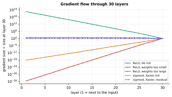
Reading it: the horizontal axis is the layer (1 is next to the input, 30 next to the loss). The vertical axis is the size of the gradient reaching that layer divided by its size at layer 30, on a log scale where each gridline is a factor of 10⁶. So every line starts at 1 on the right; read it from right to left, following backprop, and its height at layer 1 is the ratio in the table. The healthy ReLU + He line stays within a factor of about 5 of 1. The too-small line dives about 36 orders of magnitude. The sigmoid line dives too, but only about half as far, 18 orders: Xavier keeps the weights' own gain near 1, so what shrinks the gradient is sigmoid's slope, at most 0.25, about 4× per layer. The too-large line climbs about 22 orders. The dashed line is the same sigmoid network with skip connections, and it stays flat (see residual connections below).
Level 3: the formula and its symbols
$$ \text{gain per layer} \approx \sigma_w \sqrt{n_{\text{in}}}\;\cdot\;\text{typical }\phi' $$
Symbols
| Symbol | Meaning here | In the example |
|---|---|---|
| $\sigma_w$ | the standard deviation (typical size) of the random starting weights | 0.01 (too small) |
| $n_{\text{in}}$ | "fan-in": how many inputs each neuron adds up | 64 |
| $\sqrt{n_{\text{in}}}$ | a sum of $n$ random terms grows like $\sqrt{n}$, not $n$ | 8 |
| typical $\phi'$ | the average slope the activation passes back | ≈ 0.7 for ReLU's "half on" |
In words: "each layer multiplies the gradient by roughly the weight size, times the square root of how many inputs it sums, times the activation's typical slope."
With the numbers: too small: $0.01 \times 8 \times 0.7 = 0.056$ per layer, and $0.056^{30} \approx 3 \times 10^{-38}$. Too large: $1 \times 8 \times 0.7 = 5.6$ per layer, and $5.6^{30} \approx 3 \times 10^{22}$.
Level 3: in Python
In Python:
import math
n_in, typical_slope = 64, 0.7
for sigma_w in (0.01, 1.0):
    # σ_w √n_in · typical φ'
    gain = sigma_w * math.sqrt(n_in) * typical_slope
    # per layer, then over 30 layers
    print(round(gain, 3), f"{gain ** 30:.0e}")  # → 0.056 3e-38 5.6 3e+22
In code: gradient_norms runs a 30-layer, 64-wide network forward and backward and returns the gradient size reaching every layer; first_to_last_gradient_ratio divides the first by the last to fill the table.
Why it matters: you can't see this from the loss curve alone. A network whose early layers get no gradient still trains a little (the late layers learn), just badly. Plotting per-layer gradient norms is a standard diagnostic.
Initialization: setting every amplifier's volume
Think of a chain of 30 audio amplifiers. If each is set a little too quiet, the sound fades to nothing; a little too loud, and it distorts into noise. Set each so that what comes out is exactly as loud as what went in, and the music survives the whole chain. Initialization picks the random starting weights' size so that each layer passes on a signal of the same size, forward and backward.
Worked example:
| scheme | rule for the weight standard deviation | example |
|---|---|---|
| Xavier (Glorot), for tanh/sigmoid | √(2 / (fan-in + fan-out)) | 100 in, 100 out → √(2/200) = 0.1 |
| He (Kaiming), for ReLU | √(2 / fan-in) | 50 in → √(2/50) = 0.2 |
He uses twice Xavier's variance because ReLU zeroes about half its inputs, throwing away half the signal's energy; the factor 2 puts it back.
flowchart LR
  A{Activation?} -->|ReLU / GELU| He["He: std = √(2 / fan_in)"]
  A -->|tanh / sigmoid / linear| X["Xavier: std = √(2 / (fan_in + fan_out))"]
  He & X --> S[Signal keeps its size<br/>layer after layer]
Reading it: the choice of starting weights follows the activation. Both rules have the same goal, shown in the last box: a layer should neither shrink nor grow what passes through it.
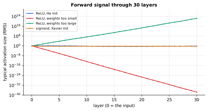
Reading it: this is the forward direction: the typical size of the activations entering each layer, log scale. With He initialization the ReLU network's signal stays near 1 for all 30 layers. Too small, it fades to nothing within a few layers; too large, it grows by about 5.6× per layer. For the three ReLU lines the backward picture above mirrors this one, because the same weights scale both directions. The sigmoid line is where the mirror breaks: its signal holds steady near 0.5 for all 30 layers (sigmoid's outputs sit around 0.5 whatever comes in), yet its gradient above lost 18 orders of magnitude. The forward pass only sends values through sigmoid; the backward pass multiplies by sigmoid's slope, at most 0.25, at every layer. A healthy forward signal does not prove a healthy gradient, so check both.
Level 3: the formula and its symbols
$$ \operatorname{Var}(z) = n_{\text{in}}\,\operatorname{Var}(w)\,\mathbb{E}[h^2] \quad\Rightarrow\quad \operatorname{Var}(w) = \frac{2}{n_{\text{in}}}\ \text{for ReLU} $$
Symbols
| Symbol | Meaning here | In the example |
|---|---|---|
| $z$ | one neuron's weighted sum | |
| $\operatorname{Var}(\cdot)$ | variance: the average squared distance from the mean (standard deviation squared) | $0.2^2 = 0.04$ |
| $w$ | one weight | |
| $h$ | one input to the neuron (the previous layer's output) | |
| $\mathbb{E}[h^2]$ | the average of $h^2$ ("E" for expected value, the long-run average) | half the pre-ReLU variance |
| $n_{\text{in}}$ | fan-in | 50 |
| $\Rightarrow$ | "therefore" |
In words: "the variance of a neuron's sum is the number of inputs times the weight variance times the average squared input; ReLU halves that average, so to keep the variance steady the weights need variance 2 over the fan-in."
With the numbers: $\operatorname{Var}(w) = 2/50 = 0.04$, so the standard deviation is $\sqrt{0.04} = 0.2$.
Level 3: in Python
In Python:
import math
n_in = 50
# Var(w) = 2 / n_in, for ReLU
var_w = 2 / n_in
# the variance, then the standard deviation
var_w, round(math.sqrt(var_w), 3)  # → (0.04, 0.2)
# Xavier for comparison: 100 in, 100 out
round(math.sqrt(2 / (100 + 100)), 3)  # → 0.1
In code: init_std returns the starting weight standard deviation for Xavier, He and two deliberately bad choices; forward_signal_rms measures the forward signal plotted above.
Why it matters: every framework initializes this way by default
(PyTorch's nn.Linear uses a Kaiming-style uniform init). Custom layers or
deep stacks built without it can silently fail to train.
Residual connections: an express lane for the gradient
Picture a building where messages go up by stairs, one floor at a time, and at every landing someone might mumble. Add an express lift that runs the whole height, and the message always arrives intact; each floor adds its own notes to what the lift carries. A residual (or skip) connection is that express lift: each block computes a correction and adds it to its input, instead of replacing the input.
Worked example: ten blocks, each with slope 0.025 of its own.
| per-block factor | after 10 blocks | |
|---|---|---|
| plain: h ← f(h) | 0.025 | 0.025¹⁰ ≈ 9.5 × 10⁻¹⁷ |
| residual: h ← h + f(h) | 1 + 0.025 | 1.025¹⁰ = 1.28 |
flowchart TD
  IN[h] --> F["block F<br/>(layers, activation)"]
  F --> ADD((+))
  IN -- "skip: identity" --> ADD
  ADD --> OUT["h + F(h)"]
Reading it: the input splits. One copy goes through the block, the other goes straight around it, and the two are added. Going backwards, the gradient also splits: one part flows back through the block (and may shrink), the other flows through the "+" untouched. That untouched path is the "1" in 1 + 0.025, and it guarantees that some gradient reaches the early layers no matter how deep the stack is.
Level 3: the formula and its symbols
$$ h_{l+1} = h_l + F(h_l), \qquad \frac{\partial h_{l+1}}{\partial h_l} = I + \frac{\partial F}{\partial h_l} $$
Symbols
| Symbol | Meaning here | In the example |
|---|---|---|
| $h_l$ | the signal entering block $l$ | |
| $F$ | what the block computes (its layers and activation) | slope 0.025 |
| $\partial h_{l+1}/\partial h_l$ | how the block's output changes with its input | $1.025$ |
| $I$ | the identity: "1" for a single number, the do-nothing matrix for vectors | 1 |
| $\partial F/\partial h_l$ | the block's own slope | 0.025 |
In words: "the output is the input plus a correction, so its slope is one plus the correction's slope, never just the correction's slope."
With the numbers: $(1 + 0.025)^{10} = 1.28$ instead of $0.025^{10} \approx 10^{-16}$.
Level 3: in Python
In Python:
# each block's own slope
dF_dh = 0.025
plain, residual = 1.0, 1.0
for l in range(10):
    # h ← F(h): the slope is just ∂F/∂h
    plain *= dF_dh
    # h ← h + F(h): the slope is I + ∂F/∂h
    residual *= 1 + dF_dh
f"{plain:.1e}", round(residual, 2)  # → ('9.5e-17', 1.28)
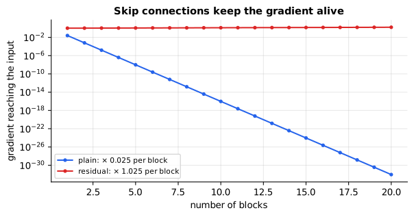
Reading it: the x-axis counts stacked blocks and the y-axis, on a log scale, is how much gradient survives the trip back to the input (1 means all of it). The plain line drops by a factor of 40 with every block, a straight plunge on a log scale, and after 10 blocks it is at 10⁻¹⁶: early layers receive essentially nothing. The residual line stays near 1 at every depth, because each block's "1 +" passes the gradient through intact. That flat line is why networks with hundreds of layers can be trained at all.
In code: residual_chain_gradient multiplies the per-block factors from the table, with or without the skip path.
Why it matters: residual connections (ResNet, 2015) made 100+ layer
networks trainable, and every transformer wraps both its attention and its
feed-forward sub-layers in one (see primer.ml.transformer). One caveat
the code shows: adding corrections forever makes the signal grow (a 30-layer
residual ReLU stack here grows its gradient about 7 million×), which is why
residuals are always paired with normalization.
Normalization: grading on a curve
A teacher can "grade on a curve" in two ways. Batch normalization curves each question across the whole class: your score on question 3 is compared with everyone else's score on question 3, so your grade depends on who else sat the exam. Layer normalization curves each student across their own answers: your scores are rescaled relative to your own average, whoever else is in the room. Both re-centre and re-scale numbers into a steady range so no layer is swamped by huge or tiny values.
Worked examples:
- BatchNorm, batch [[1, 2], [3, 6]]: column means (2, 4), standard deviations (1, 2), so the output is [[−1, −1], [1, 1]]. The value 1 becomes −1.22 in the batch (1, 3, 5) but −0.93 in the batch (1, 3, 11).
- LayerNorm, one row (1, 2, 3, 4): mean 2.5, standard deviation 1.118, so the output is (−1.342, −0.447, 0.447, 1.342), whatever else is in the batch.
- RMSNorm, the same row: root-mean-square √((1+4+9+16)/4) = 2.739, so the output is (0.365, 0.730, 1.095, 1.461). No mean is subtracted.
flowchart LR
  subgraph M["activations: rows = examples, columns = features"]
    direction TB
    r1["ex 1: a  b  c  d"]
    r2["ex 2: e  f  g  h"]
    r3["ex 3: i  j  k  l"]
  end
  M -->|"down each column<br/>(across the batch)"| BN[BatchNorm]
  M -->|"along each row<br/>(within one example)"| LN[LayerNorm / RMSNorm]
Reading it: the same grid of activations can be normalized in two directions. BatchNorm takes statistics down each column, across the examples, so every example's output depends on its batch-mates. LayerNorm and RMSNorm take statistics along each row, within a single example, so an example is normalized the same way alone or in any batch.
Level 3: the formula and its symbols
$$ \text{LayerNorm}(x) = \gamma \odot \frac{x - \mu}{\sqrt{\sigma^2 + \epsilon}} + \beta, \qquad \text{RMSNorm}(x) = \gamma \odot \frac{x}{\sqrt{\tfrac{1}{d}\sum_{i=1}^{d} x_i^2 + \epsilon}} $$
Symbols
| Symbol | Meaning here | In the example |
|---|---|---|
| $x$ | one example's activations (a row) | (1, 2, 3, 4) |
| $d$ | number of features in the row | 4 |
| $x_i$ | the $i$-th feature | $x_4 = 4$ |
| $\mu$ | "mu", the row's mean | 2.5 |
| $\sigma^2$ | "sigma squared", the row's variance | 1.25 |
| $\epsilon$ | a tiny number so we never divide by zero | $10^{-5}$ |
| $\gamma, \beta$ | "gamma, beta", a learned scale and shift per feature, so the network can undo the normalization if it helps | 1 and 0 at the start |
| $\odot$ | multiply feature by feature |
In words: "LayerNorm subtracts the row's mean, divides by its standard deviation, then applies a learned scale and shift; RMSNorm skips the mean and just divides by the root-mean-square."
With the numbers: LayerNorm: $(4 - 2.5)/\sqrt{1.25} = 1.5/1.118 = 1.342$. RMSNorm: $4 / \sqrt{7.5} = 4/2.739 = 1.461$.
BatchNorm is the column version of the same formula, with $\mu$ and $\sigma^2$ computed across the batch for each feature.
Level 3: in Python
In Python:
import math
x = [1, 2, 3, 4]
d, eps, gamma, beta = len(x), 1e-5, 1.0, 0.0
# the row's mean
mu = sum(x) / d
# σ², the row's variance
var = sum((x_i - mu) ** 2 for x_i in x) / d
mu, var  # → (2.5, 1.25)
# LayerNorm
[round(gamma * (x_i - mu) / math.sqrt(var + eps) + beta, 3) for x_i in x]  # → [-1.342, -0.447, 0.447, 1.342]
# √((1/d) Σ x_i² + ε)
rms = math.sqrt(sum(x_i ** 2 for x_i in x) / d + eps)
round(rms, 3)  # → 2.739
# RMSNorm: no mean subtracted
[round(gamma * x_i / rms, 3) for x_i in x]  # → [0.365, 0.73, 1.095, 1.461]
In code: batch_norm normalizes each column across the batch, layer_norm each row across its own features, and rms_norm divides each row by its root-mean-square.
Why it matters: transformers use LayerNorm or RMSNorm, never BatchNorm: sequences have different lengths, batches at inference are often size 1, and an example's output must not depend on its batch-mates. Modern LLMs (Llama and others) use RMSNorm because it's cheaper and works as well, and they place it before each sub-layer ("pre-norm"), which keeps the residual path clean and trains more stably. CNNs are where BatchNorm lives on: ResNet puts it after every convolution.
Gradient clipping: a circuit breaker
Even with all of the above, one unlucky batch can produce a gradient spike. A circuit breaker doesn't stop the current; it caps it. Clipping by global norm does the same to the update: if the gradient's total length exceeds a limit, it's scaled down to the limit, direction unchanged.
Worked example: in the exploding (too-large) 30-layer network above, the gradients' combined length is astronomically large. Clipped with a limit of 1, the update has length exactly 1 and points the same way.
flowchart LR
  G[Gradients of all layers] --> N["‖g‖: combined length"]
  N --> C{"above the limit?"}
  C -->|yes| S["scale every gradient by limit / ‖g‖"]
  C -->|no| K[leave unchanged]
Reading it: measure all layers' gradients together as one long list; if that list is longer than the limit, shrink every entry by the same factor.
Level 3: the formula and its symbols
$$ g \leftarrow g \cdot \min!\left(1, \frac{c}{\lVert g \rVert}\right) $$
Symbols
| Symbol | Meaning here | In the example |
|---|---|---|
| $g$ | every weight gradient, as one long list | the 30 layers' gradients |
| $\lVert g \rVert$ | its length: square every entry, add them up, take the square root | enormous |
| $c$ | the limit | 1 |
In words: "if the gradient is longer than the limit, rescale it to the limit."
With the numbers: in the too-large network $\lVert g \rVert \approx 8 \times 10^{46}$;
with $c = 1$ every entry is multiplied by about $10^{-47}$ and the new length
is exactly 1. (The
optimizers lesson traces (3, 4) → (0.6, 0.8); see
primer.ml.optimizers.clip_by_global_norm, which this lesson reuses.)
Level 3: in Python
In Python:
import math
# a stand-in with the same enormous length
g = [4.8e46, 6.4e46]
# ‖g‖
norm = math.sqrt(sum(g_i ** 2 for g_i in g))
f"{norm:.0e}"  # → '8e+46'
c = 1
# min(1, c / ‖g‖)
scale = min(1, c / norm)
f"{scale:.0e}"  # → '1e-47'
# the new length
round(math.sqrt(sum((g_i * scale) ** 2 for g_i in g)), 6)  # → 1.0
In code: layer_gradients collects every layer's weight gradient from a 30-layer network, and global_norm_after_clipping reports their combined length after clipping.
Why it matters: clipping treats the symptom, not the cause: it makes a rare spike harmless, but a network that explodes on every step needs better initialization or normalization. Almost every large training run clips at a norm of about 1.
In 20 seconds
- Backprop multiplies one slope per layer, so gradients shrink (vanish) or grow (explode) exponentially with depth.
- Initialization sets weight sizes so each layer preserves signal size: Xavier for tanh/sigmoid, He (2 / fan-in) for ReLU.
- Residual connections add the input back, giving the gradient a path multiplied by 1; they're why very deep nets and transformers train.
- Normalization keeps activations in a steady range: BatchNorm across the batch (CNNs), LayerNorm/RMSNorm within each example (transformers).
- Gradient clipping caps rare spikes.
Self-test questions
Why do gradients vanish in deep sigmoid networks? Backprop multiplies the gradient by each layer's slope, and sigmoid's slope is at most 0.25. Thirty layers can shrink it by 0.25³⁰, so early layers stop learning.
What's the difference between Xavier and He initialization? Both choose the weight variance so signal size is preserved. Xavier uses 2 / (fan-in + fan-out), suited to symmetric activations like tanh. He uses 2 / fan-in, doubling the variance to compensate for ReLU zeroing half its inputs.
How do residual connections fix vanishing gradients? The block's output is input + F(input), so its derivative is 1 + F′. The gradient always has an identity path back to early layers that isn't multiplied by small slopes.
Why do transformers use LayerNorm instead of BatchNorm? BatchNorm's statistics come from the batch, which breaks for variable-length sequences, tiny or single-example batches at inference, and makes an example's output depend on its batch-mates. LayerNorm normalizes each token across its own features, independent of the batch.
What is RMSNorm and why do modern LLMs use it? LayerNorm without the mean subtraction and shift: divide by the root-mean-square and apply a learned scale. It's cheaper and trains as well.
Gradient clipping or better initialization: which fixes exploding gradients? Initialization (and normalization) fix the cause, keeping per-layer gain near 1. Clipping is a safety net for occasional spikes.
The papers behind this lesson
- Bengio, Simard & Frasconi, Learning long-term dependencies with gradient descent is difficult (IEEE Trans. Neural Networks, 1994): https://doi.org/10.1109/72.279181 Proved that gradients shrink or explode exponentially through many steps, the root of the problem.
- Glorot & Bengio, Understanding the difficulty of training deep feedforward neural networks (AISTATS 2010): https://proceedings.mlr.press/v9/glorot10a.html Diagnosed saturation and derived Xavier initialization to keep variance steady across layers.
- He, Zhang, Ren & Sun, Delving Deep into Rectifiers (2015): https://arxiv.org/abs/1502.01852 Derived the 2 / fan-in (He) initialization for ReLU networks.
- He, Zhang, Ren & Sun, Deep Residual Learning for Image Recognition (2015): https://arxiv.org/abs/1512.03385 Introduced residual connections and trained networks over 100 layers deep. annotated companion
- Ioffe & Szegedy, Batch Normalization (2015): https://arxiv.org/abs/1502.03167 Normalized activations across the batch, allowing much higher learning rates.
- Ba, Kiros & Hinton, Layer Normalization (2016): https://arxiv.org/abs/1607.06450 Normalized within each example instead, independent of batch size; the version transformers use. annotated companion
- Zhang & Sennrich, Root Mean Square Layer Normalization (2019): https://arxiv.org/abs/1910.07467 Dropped LayerNorm's mean subtraction for a cheaper normalization with the same benefit.
- Xiong et al., On Layer Normalization in the Transformer Architecture (2020): https://arxiv.org/abs/2002.04745 Showed why putting the norm before each sub-layer (pre-norm) trains more stably.
Further reading
- CS231n notes, Neural Networks Part 2 (initialization, batch norm): https://cs231n.github.io/neural-networks-2/
- Michael Nielsen, Why are deep neural networks hard to train?: http://neuralnetworksanddeeplearning.com/chap5.html
- Goodfellow, Bengio & Courville, Deep Learning, ch. 8 (optimization for training deep models): https://www.deeplearningbook.org/contents/optimization.html
- PyTorch
nn.initdocs: https://pytorch.org/docs/stable/nn.init.html - PyTorch
nn.LayerNorm: https://pytorch.org/docs/stable/generated/torch.nn.LayerNorm.html
1r""" 2# Deep networks: why deep stacks fail to train, and the fixes that made them work 3 4Run: `python -m primer.ml.deep_nets` 5 6New to the notation (Π, ∂, σ)? `primer.notation` builds every symbol used 7here from zero. This lesson builds on backpropagation from 8`primer.ml.neural_net` and the optimizer step from `primer.ml.optimizers`. 9 10## Level 1: The practitioner's guide 11 12**In one sentence.** Backpropagation multiplies one factor per layer, so 13in a deep stack the learning signal shrinks to nothing or grows without 14bound unless every layer is built to pass it on at about its original 15size, and the four standard fixes (a good activation, matched 16initialization, residual connections, normalization) plus a safety net 17(gradient clipping) are what make every modern architecture trainable. 18 19**When you need it.** You need this when you read a model's config and 20meet `rms_norm_eps`, `initializer_range` or `layer_norm_eps`, when a 21network you built stops improving while its loss curve looks merely slow, 22when a training run turns NaN in its first steps, or when a paper says 23"pre-norm" and you have to decide whether it matters. The tell: a model 24whose late layers learn while its early layers stay at their random start, 25which no loss curve shows and a plot of gradient size per layer shows at 26once. You don't need it to fine-tune a published transformer: the fixes 27are baked into its architecture, and your job is to leave them alone. One 28number from this lesson says why they are there: in a 30-layer network of 29ReLU units, weights drawn a little too small shrink the gradient reaching 30the first layer by 36 orders of magnitude, a little too large grow it by 3122, and the right size keeps it within a factor of about 4. 32 33**Your options.** The fixes, from the ones a framework applies for you to 34the ones that shape an architecture: 35 36| Option | What it does | What it guarantees | What it costs | Where it lives | 37|---|---|---|---|---| 38| An activation with slope near 1 (ReLU exactly; GELU and SiLU for large positive inputs) | Passes the gradient through unshrunk for positive inputs, where sigmoid passes at most 0.25 (GELU and SiLU pass 0.5 at zero, rising toward 1) | No 0.25-per-layer decay: ten sigmoid layers lose a factor of a million, ten ReLU layers lose nothing | ReLU units pushed negative pass nothing and can die; GELU and SiLU leak a little instead | `hidden_act` in a config | 39| Initialization matched to the activation (Xavier, He) | Sets the starting weights' size so each layer passes signal on at the same size, forward and backward | The healthy line in this lesson's figure: a factor of about 4 over 30 layers, against 10⁻³⁶ or 10²² | Nothing at runtime; a per-layer rule you must apply to custom layers | The framework's default init; `initializer_range` in a config | 40| Residual connections | Each block adds its correction to its input instead of replacing it | Some gradient always reaches the early layers: 1.28 after ten blocks against 10⁻¹⁶ without | The signal grows as corrections pile up (7 million times over 30 layers here) unless normalized; block input and output must share a shape | The architecture: every transformer block | 41| Normalization (BatchNorm, LayerNorm, RMSNorm) | Re-centres and rescales activations, across the batch or within each example | Activations in a steady range at every depth; with residuals, a stable stack of any depth | A mean and a variance per layer per step (RMSNorm drops the mean); BatchNorm ties each example to its batch-mates | The architecture: `layer_norm_eps`, `rms_norm_eps` | 42| Gradient clipping | Rescales the whole update when its length exceeds a limit | A rare spike cannot wreck the run: a gradient of length 8 × 10⁴⁶ becomes length 1, same direction | One norm per step; a network that explodes every step is hidden, not fixed | The training loop: `max_grad_norm` | 43 44**How to choose.** Start from whether you are reading an architecture or 45building one. 46 47- Fine-tuning a published model: read the config and change nothing. A 48 Llama model is built with RMSNorm placed before each sub-layer 49 (pre-norm), residuals in every block and SiLU-based activations, and its 50 released config records the numbers, such as Llama 2's `rms_norm_eps` of 51 10⁻⁵; the trained weights assume every one of them. 52- Building a network more than a few layers deep: ReLU or GELU, the 53 framework's default initialization (PyTorch's `nn.Linear` scales its 54 starting weights by the fan-in), a residual path around every block, and 55 a normalization layer beside it. 56- Sequences, or inference one example at a time: LayerNorm or RMSNorm, 57 never BatchNorm, because an example's output must not depend on who else 58 is in the batch. Convolutional networks with large batches: BatchNorm, 59 which ResNet places after every convolution. 60- A run that spikes: clip at 1.0, the limit GPT-3 and Llama 2 trained with. 61 If the clip fires on every step, the fault is initialization or 62 normalization, and clipping is masking it. 63- A network that trains slowly for no visible reason: plot the gradient 64 norm per layer. Vanishing shows up as a slope of many orders of 65 magnitude from the last layer to the first. 66- Whatever you pick, the goal is one number: a per-layer factor near 1 in 67 both directions. Check the forward signal and the backward gradient 68 separately, because a healthy one does not prove a healthy other. 69 70**What it costs.** Initialization is free. Residual connections cost one 71addition per value, nothing beside the block's matrix multiplies, but fix 72the shape of every block's output to its input. A 73normalization layer costs a mean and a variance per row per layer, which 74is why RMSNorm, dropping the mean, is the cheaper choice modern language 75models make. Clipping costs one norm over all parameters per step. What they buy is depth itself: ResNet trained networks over 100 76layers deep with residuals, a 7-billion-parameter Llama config stacks 32 77blocks, and Llama 3's largest model is a dense transformer with 405 billion 78parameters, none of which could be trained if the per-layer factor drifted 79from 1. Depth is also what you pay for at inference: every layer runs on 80every token. 81 82**What breaks.** 83 84- **Early layers never learn.** The gradient vanished on the way back: 85 sigmoid or tanh stacked deep (18 orders of magnitude lost over 30 layers 86 even with Xavier initialization), or weights initialized too small. 87- **NaN in the first steps.** Weights too large (22 orders of magnitude 88 of growth), or residual blocks stacked without normalization. 89- **A healthy forward pass with a dead backward pass.** The sigmoid 90 network's signal holds steady near 0.5 through all 30 layers while its 91 gradient collapses, because the forward pass sends values through the 92 activation and the backward pass multiplies by its slope. Check both. 93- **BatchNorm where the batch is not a population.** The value 1 becomes 94 −1.22 in one batch and −0.93 in another; at batch size 1, or with 95 variable-length sequences, the statistics are meaningless. Use LayerNorm. 96- **A custom layer that silently fails to train.** It skipped the 97 initialization rule the framework applies to its own layers. 98- **Clipping that fires every step.** Not a spike: an explosion. Fix the 99 cause. 100- **Post-norm instability.** Placing the norm after the residual add trains 101 less stably than before it (Xiong et al., 2020); pre-norm is what Llama 102 and most recent models use. 103 104**In the wild.** Llama 2's paper describes its blocks as pre-normalization 105with RMSNorm, the SwiGLU activation and rotary position embeddings, and 106Hugging Face's `LlamaConfig` exposes the settings (`initializer_range` 1070.02, `num_hidden_layers` 32, `hidden_act` silu, and an `rms_norm_eps` that 108defaults to 1e-6 while Meta's Llama 2 code and released config use 1e-5). 109PyTorch's `nn.LayerNorm` takes the shape to normalize over with 110`eps=1e-05` and a learned per-element scale and shift; its `nn.Linear` 111initializes from a uniform range set by the fan-in; and 112`torch.nn.utils.clip_grad_norm_` clips by the norm over all parameters 113together, which Hugging Face's `TrainingArguments` calls with a default 114`max_grad_norm` of 1.0, the same limit Llama 2 trained with. The fixes are 115He et al. (ResNet and He initialization, 2015), Glorot and Bengio (Xavier, 1162010), Ioffe and Szegedy (BatchNorm, 2015), Ba, Kiros and Hinton 117(LayerNorm, 2016) and Zhang and Sennrich (RMSNorm, 2019), with the problem 118itself diagnosed by Bengio, Simard and Frasconi (1994); all are linked at 119the end of the lesson. 120 121**Go deeper.** Level 2 multiplies the slopes of a ten-layer chain by hand, 122watches the gradient at every layer of a 30-layer network under four 123initializations, derives the Xavier and He rules from one variance 124equation, shows the "1 +" that residual connections add, normalizes one 125row three ways with the numbers shown, and clips an exploding gradient of 126length 8 × 10⁴⁶ down to 1. If you only needed to read a config, you are 127done. 128 129## Level 2: How it works, from scratch 130 131A deep network's gradient is a product with one factor per layer, and 132every fix in this lesson is a way of holding that factor near 1. This 133level builds the problem in a chain of ten numbers, watches it in a 13430-layer network, then adds each fix and measures what it restores. 135 136## The idea: a gradient is a product of slopes 137 138Picture a game of telephone along a line of 30 people. Each person repeats 139the message to the next, but everyone speaks at a quarter of the volume they 140heard. By the end of the line the message is silence. If instead everyone 141speaks 1.5× louder, the end of the line is a deafening roar. Training a deep 142network has exactly this problem, run backwards: the learning signal (the 143**gradient**, how much each weight should change; see `primer.ml.neural_net`) 144starts at the output and is passed back layer by layer, and each layer 145multiplies it by its own **slope** (derivative). Thirty multiplications by 146something below 1 is almost zero: the **vanishing gradient**. Thirty by 147something above 1 is enormous: the **exploding gradient**. 148 149Worked example: a chain of ten one-number layers, each sitting at its 150steepest point. 151 152| chain | slope per layer | gradient after 10 layers | 153|---|---|---| 154| sigmoid units, weight 1 | 0.25 | 0.25¹⁰ = 0.00000095 | 155| linear units, weight 1 | 1 | 1¹⁰ = 1 | 156| linear units, weight 1.5 | 1.5 | 1.5¹⁰ = 57.7 | 157 158```mermaid 159flowchart RL 160 L[Loss] -- "gradient 1" --> H10[layer 10] 161 H10 -- "× 0.25" --> H9[layer 9] 162 H9 -- "× 0.25" --> H8[layer 8] 163 H8 -- "× 0.25 ... " --> H2[layer 2] 164 H2 -- "× 0.25" --> H1["layer 1<br/>receives 0.25¹⁰ ≈ 1e-6"] 165``` 166 167**Reading it:** read right to left, the direction backprop travels. The loss 168hands the last layer a gradient of 1. Every hop multiplies by that layer's 169slope (0.25 for a sigmoid at its steepest). After ten hops the first layer 170receives about one millionth of the signal, so its weights barely change: it 171effectively stops learning while the later layers carry on. 172 173$$ 174\frac{\partial \mathcal{L}}{\partial h_0} = \frac{\partial \mathcal{L}}{\partial h_L}\prod_{l=1}^{L} w_l\,\phi'(z_l) 175$$ 176 177**Symbols** 178 179| Symbol | Meaning here | In the example | 180|---|---|---| 181| $h_0$ | the input to the first layer | | 182| $h_L$ | the output of the last layer | | 183| $L$ | the number of layers | 10 | 184| $l$ | a counter over the layers | 1 to 10 | 185| $\prod_{l=1}^{L}$ | "multiply together the following, for every layer" (like Σ, but multiplying) | ten factors | 186| $w_l$ | layer $l$'s weight | 1 | 187| $\phi'(z_l)$ | the activation's slope at layer $l$'s input | 0.25 | 188| $\partial \mathcal{L}/\partial h$ | how much the loss changes when $h$ changes | 1 at the top | 189 190**In words:** "the gradient reaching the first layer is the gradient at the 191top times every layer's weight times every layer's slope." 192 193**With the numbers:** $1 \times (1 \times 0.25)^{10} = 9.5 \times 10^{-7}$. 194 195**In Python:** 196 197```python 198def gradient_at_input(w_l, slope, L=10): 199 # ∂L/∂h_L: the loss hands the top layer 1 200 grad = 1.0 201 # Π over the layers: a running product 202 for l in range(L): 203 # × w_l φ'(z_l) 204 grad *= w_l * slope 205 return grad 206# sigmoid at its steepest 207f"{gradient_at_input(1, 0.25):.1e}" # → '9.5e-07' 208# linear, weight 1 209gradient_at_input(1, 1) # → 1.0 210# linear, weight 1.5 211round(gradient_at_input(1.5, 1), 1) # → 57.7 212``` 213 214`chain_gradient` builds that chain and backprops through it. 215 216**Why it matters:** this is why networks deeper than a handful of layers 217were considered untrainable for decades. Every fix below (better 218activations, careful initialization, residual connections, normalization) 219is a way of keeping the per-layer factor close to 1. 220 221## In a real network: watching the gradient layer by layer 222 223In a real layer, each neuron sums 64 inputs, so the multiplier per layer 224depends on three things together: the size of the weights, how many inputs 225each neuron adds up, and the activation's slope. Same telephone game, but 226now everyone in the line hears 64 people at once. 227 228Worked example: a 30-layer network, 64 neurons per layer. The ratio of the 229gradient at the first layer to the gradient at the last: 230 231| setup | ratio first / last | 232|---|---| 233| ReLU, He initialization | ≈ 4 (healthy) | 234| ReLU, weights too small (std 0.01) | ≈ 10⁻³⁶ (vanished) | 235| ReLU, weights too large (std 1) | ≈ 10²² (exploded) | 236| sigmoid, Xavier initialization | ≈ 10⁻¹⁸ (vanished) | 237 238 239 240**Reading it:** the horizontal axis is the layer (1 is next to the input, 30 241next to the loss). The vertical axis is the size of the gradient reaching 242that layer divided by its size at layer 30, on a log scale where each 243gridline is a factor of 10⁶. So every line starts at 1 on the right; read it 244from right to left, following backprop, and its height at layer 1 is the 245ratio in the table. The healthy ReLU + He line stays within a factor of 246about 5 of 1. The too-small line dives about 36 orders of magnitude. The 247sigmoid line dives too, but only about half as far, 18 orders: Xavier keeps 248the weights' own gain near 1, so what shrinks the gradient is sigmoid's 249slope, at most 0.25, about 4× per layer. The too-large line climbs about 22 250orders. The dashed line is the same sigmoid network with skip connections, 251and it stays flat (see residual connections below). 252 253$$ 254\text{gain per layer} \approx \sigma_w \sqrt{n_{\text{in}}}\;\cdot\;\text{typical }\phi' 255$$ 256 257**Symbols** 258 259| Symbol | Meaning here | In the example | 260|---|---|---| 261| $\sigma_w$ | the standard deviation (typical size) of the random starting weights | 0.01 (too small) | 262| $n_{\text{in}}$ | "fan-in": how many inputs each neuron adds up | 64 | 263| $\sqrt{n_{\text{in}}}$ | a sum of $n$ random terms grows like $\sqrt{n}$, not $n$ | 8 | 264| typical $\phi'$ | the average slope the activation passes back | ≈ 0.7 for ReLU's "half on" | 265 266**In words:** "each layer multiplies the gradient by roughly the weight 267size, times the square root of how many inputs it sums, times the 268activation's typical slope." 269 270**With the numbers:** too small: $0.01 \times 8 \times 0.7 = 0.056$ 271per layer, and $0.056^{30} \approx 3 \times 10^{-38}$. Too large: 272$1 \times 8 \times 0.7 = 5.6$ per layer, and $5.6^{30} \approx 3 \times 10^{22}$. 273 274**In Python:** 275 276```python 277import math 278n_in, typical_slope = 64, 0.7 279for sigma_w in (0.01, 1.0): 280 # σ_w √n_in · typical φ' 281 gain = sigma_w * math.sqrt(n_in) * typical_slope 282 # per layer, then over 30 layers 283 print(round(gain, 3), f"{gain ** 30:.0e}") # → 0.056 3e-38 5.6 3e+22 284``` 285 286**In code:** `gradient_norms` runs a 30-layer, 64-wide network forward and backward and returns the gradient size reaching every layer; `first_to_last_gradient_ratio` divides the first by the last to fill the table. 287 288**Why it matters:** you can't see this from the loss curve alone. A network 289whose early layers get no gradient still trains a little (the late layers 290learn), just badly. Plotting per-layer gradient norms is a standard 291diagnostic. 292 293## Initialization: setting every amplifier's volume 294 295Think of a chain of 30 audio amplifiers. If each is set a little too quiet, 296the sound fades to nothing; a little too loud, and it distorts into noise. 297Set each so that what comes out is exactly as loud as what went in, and the 298music survives the whole chain. **Initialization** picks the random 299starting weights' size so that each layer passes on a signal of the same 300size, forward and backward. 301 302Worked example: 303 304| scheme | rule for the weight standard deviation | example | 305|---|---|---| 306| Xavier (Glorot), for tanh/sigmoid | √(2 / (fan-in + fan-out)) | 100 in, 100 out → √(2/200) = **0.1** | 307| He (Kaiming), for ReLU | √(2 / fan-in) | 50 in → √(2/50) = **0.2** | 308 309He uses twice Xavier's variance because ReLU zeroes about half its inputs, 310throwing away half the signal's energy; the factor 2 puts it back. 311 312```mermaid 313flowchart LR 314 A{Activation?} -->|ReLU / GELU| He["He: std = √(2 / fan_in)"] 315 A -->|tanh / sigmoid / linear| X["Xavier: std = √(2 / (fan_in + fan_out))"] 316 He & X --> S[Signal keeps its size<br/>layer after layer] 317``` 318 319**Reading it:** the choice of starting weights follows the activation. Both 320rules have the same goal, shown in the last box: a layer should neither 321shrink nor grow what passes through it. 322 323 324 325**Reading it:** this is the forward direction: the typical size of the 326activations entering each layer, log scale. With He initialization the ReLU 327network's signal stays near 1 for all 30 layers. Too small, it fades to 328nothing within a few layers; too large, it grows by about 5.6× per layer. 329For the three ReLU lines the backward picture above mirrors this one, 330because the same weights scale both directions. The sigmoid line is where 331the mirror breaks: its signal holds steady near 0.5 for all 30 layers 332(sigmoid's outputs sit around 0.5 whatever comes in), yet its gradient 333above lost 18 orders of magnitude. The forward pass only sends values 334through sigmoid; the backward pass multiplies by sigmoid's slope, at most 3350.25, at every layer. A healthy forward signal does not prove a healthy 336gradient, so check both. 337 338$$ 339\operatorname{Var}(z) = n_{\text{in}}\,\operatorname{Var}(w)\,\mathbb{E}[h^2] 340\quad\Rightarrow\quad 341\operatorname{Var}(w) = \frac{2}{n_{\text{in}}}\ \text{for ReLU} 342$$ 343 344**Symbols** 345 346| Symbol | Meaning here | In the example | 347|---|---|---| 348| $z$ | one neuron's weighted sum | | 349| $\operatorname{Var}(\cdot)$ | variance: the average squared distance from the mean (standard deviation squared) | $0.2^2 = 0.04$ | 350| $w$ | one weight | | 351| $h$ | one input to the neuron (the previous layer's output) | | 352| $\mathbb{E}[h^2]$ | the average of $h^2$ ("E" for expected value, the long-run average) | half the pre-ReLU variance | 353| $n_{\text{in}}$ | fan-in | 50 | 354| $\Rightarrow$ | "therefore" | | 355 356**In words:** "the variance of a neuron's sum is the number of inputs times 357the weight variance times the average squared input; ReLU halves that 358average, so to keep the variance steady the weights need variance 2 over 359the fan-in." 360 361**With the numbers:** $\operatorname{Var}(w) = 2/50 = 0.04$, so the standard 362deviation is $\sqrt{0.04} = 0.2$. 363 364**In Python:** 365 366```python 367import math 368n_in = 50 369# Var(w) = 2 / n_in, for ReLU 370var_w = 2 / n_in 371# the variance, then the standard deviation 372var_w, round(math.sqrt(var_w), 3) # → (0.04, 0.2) 373# Xavier for comparison: 100 in, 100 out 374round(math.sqrt(2 / (100 + 100)), 3) # → 0.1 375``` 376 377**In code:** `init_std` returns the starting weight standard deviation for Xavier, He and two deliberately bad choices; `forward_signal_rms` measures the forward signal plotted above. 378 379**Why it matters:** every framework initializes this way by default 380(PyTorch's `nn.Linear` uses a Kaiming-style uniform init). Custom layers or 381deep stacks built without it can silently fail to train. 382 383## Residual connections: an express lane for the gradient 384 385Picture a building where messages go up by stairs, one floor at a time, and 386at every landing someone might mumble. Add an express lift that runs the 387whole height, and the message always arrives intact; each floor adds its 388own notes to what the lift carries. A **residual** (or skip) connection is 389that express lift: each block computes a correction and *adds* it to its 390input, instead of replacing the input. 391 392Worked example: ten blocks, each with slope 0.025 of its own. 393 394| | per-block factor | after 10 blocks | 395|---|---|---| 396| plain: h ← f(h) | 0.025 | 0.025¹⁰ ≈ 9.5 × 10⁻¹⁷ | 397| residual: h ← h + f(h) | 1 + 0.025 | 1.025¹⁰ = 1.28 | 398 399```mermaid 400flowchart TD 401 IN[h] --> F["block F<br/>(layers, activation)"] 402 F --> ADD((+)) 403 IN -- "skip: identity" --> ADD 404 ADD --> OUT["h + F(h)"] 405``` 406 407**Reading it:** the input splits. One copy goes through the block, the 408other goes straight around it, and the two are added. Going backwards, the 409gradient also splits: one part flows back through the block (and may 410shrink), the other flows through the "+" untouched. That untouched path is 411the "1" in 1 + 0.025, and it guarantees that some gradient reaches the 412early layers no matter how deep the stack is. 413 414$$ 415h_{l+1} = h_l + F(h_l), \qquad 416\frac{\partial h_{l+1}}{\partial h_l} = I + \frac{\partial F}{\partial h_l} 417$$ 418 419**Symbols** 420 421| Symbol | Meaning here | In the example | 422|---|---|---| 423| $h_l$ | the signal entering block $l$ | | 424| $F$ | what the block computes (its layers and activation) | slope 0.025 | 425| $\partial h_{l+1}/\partial h_l$ | how the block's output changes with its input | $1.025$ | 426| $I$ | the identity: "1" for a single number, the do-nothing matrix for vectors | 1 | 427| $\partial F/\partial h_l$ | the block's own slope | 0.025 | 428 429**In words:** "the output is the input plus a correction, so its slope is 430one plus the correction's slope, never just the correction's slope." 431 432**With the numbers:** $(1 + 0.025)^{10} = 1.28$ instead of 433$0.025^{10} \approx 10^{-16}$. 434 435**In Python:** 436 437```python 438# each block's own slope 439dF_dh = 0.025 440plain, residual = 1.0, 1.0 441for l in range(10): 442 # h ← F(h): the slope is just ∂F/∂h 443 plain *= dF_dh 444 # h ← h + F(h): the slope is I + ∂F/∂h 445 residual *= 1 + dF_dh 446f"{plain:.1e}", round(residual, 2) # → ('9.5e-17', 1.28) 447``` 448 449 450 451**Reading it:** the x-axis counts stacked blocks and the y-axis, on a log 452scale, is how much gradient survives the trip back to the input (1 means 453all of it). The plain line drops by a factor of 40 with every block, a 454straight plunge on a log scale, and after 10 blocks it is at 10⁻¹⁶: early 455layers receive essentially nothing. The residual line stays near 1 at every 456depth, because each block's "1 +" passes the gradient through intact. That 457flat line is why networks with hundreds of layers can be trained at all. 458 459**In code:** `residual_chain_gradient` multiplies the per-block factors from the table, with or without the skip path. 460 461**Why it matters:** residual connections (ResNet, 2015) made 100+ layer 462networks trainable, and every transformer wraps both its attention and its 463feed-forward sub-layers in one (see `primer.ml.transformer`). One caveat 464the code shows: adding corrections forever makes the signal grow (a 30-layer 465residual ReLU stack here grows its gradient about 7 million×), which is why 466residuals are always paired with normalization. 467 468## Normalization: grading on a curve 469 470A teacher can "grade on a curve" in two ways. **Batch normalization** curves 471each question across the whole class: your score on question 3 is compared 472with everyone else's score on question 3, so your grade depends on who else 473sat the exam. **Layer normalization** curves each student across their own 474answers: your scores are rescaled relative to your own average, whoever 475else is in the room. Both re-centre and re-scale numbers into a steady range 476so no layer is swamped by huge or tiny values. 477 478Worked examples: 479 480- **BatchNorm**, batch [[1, 2], [3, 6]]: column means (2, 4), standard 481 deviations (1, 2), so the output is [[−1, −1], [1, 1]]. The value 1 becomes 482 −1.22 in the batch (1, 3, 5) but −0.93 in the batch (1, 3, 11). 483- **LayerNorm**, one row (1, 2, 3, 4): mean 2.5, standard deviation 1.118, so 484 the output is (−1.342, −0.447, 0.447, 1.342), whatever else is in the batch. 485- **RMSNorm**, the same row: root-mean-square √((1+4+9+16)/4) = 2.739, so the 486 output is (0.365, 0.730, 1.095, 1.461). No mean is subtracted. 487 488```mermaid 489flowchart LR 490 subgraph M["activations: rows = examples, columns = features"] 491 direction TB 492 r1["ex 1: a b c d"] 493 r2["ex 2: e f g h"] 494 r3["ex 3: i j k l"] 495 end 496 M -->|"down each column<br/>(across the batch)"| BN[BatchNorm] 497 M -->|"along each row<br/>(within one example)"| LN[LayerNorm / RMSNorm] 498``` 499 500**Reading it:** the same grid of activations can be normalized in two 501directions. BatchNorm takes statistics down each column, across the 502examples, so every example's output depends on its batch-mates. LayerNorm 503and RMSNorm take statistics along each row, within a single example, so an 504example is normalized the same way alone or in any batch. 505 506$$ 507\text{LayerNorm}(x) = \gamma \odot \frac{x - \mu}{\sqrt{\sigma^2 + \epsilon}} + \beta, 508\qquad 509\text{RMSNorm}(x) = \gamma \odot \frac{x}{\sqrt{\tfrac{1}{d}\sum_{i=1}^{d} x_i^2 + \epsilon}} 510$$ 511 512**Symbols** 513 514| Symbol | Meaning here | In the example | 515|---|---|---| 516| $x$ | one example's activations (a row) | (1, 2, 3, 4) | 517| $d$ | number of features in the row | 4 | 518| $x_i$ | the $i$-th feature | $x_4 = 4$ | 519| $\mu$ | "mu", the row's mean | 2.5 | 520| $\sigma^2$ | "sigma squared", the row's variance | 1.25 | 521| $\epsilon$ | a tiny number so we never divide by zero | $10^{-5}$ | 522| $\gamma, \beta$ | "gamma, beta", a learned scale and shift per feature, so the network can undo the normalization if it helps | 1 and 0 at the start | 523| $\odot$ | multiply feature by feature | | 524 525**In words:** "LayerNorm subtracts the row's mean, divides by its standard 526deviation, then applies a learned scale and shift; RMSNorm skips the mean 527and just divides by the root-mean-square." 528 529**With the numbers:** LayerNorm: $(4 - 2.5)/\sqrt{1.25} = 1.5/1.118 = 1.342$. 530RMSNorm: $4 / \sqrt{7.5} = 4/2.739 = 1.461$. 531 532BatchNorm is the column version of the same formula, with $\mu$ and 533$\sigma^2$ computed across the batch for each feature. 534 535**In Python:** 536 537```python 538import math 539x = [1, 2, 3, 4] 540d, eps, gamma, beta = len(x), 1e-5, 1.0, 0.0 541# the row's mean 542mu = sum(x) / d 543# σ², the row's variance 544var = sum((x_i - mu) ** 2 for x_i in x) / d 545mu, var # → (2.5, 1.25) 546# LayerNorm 547[round(gamma * (x_i - mu) / math.sqrt(var + eps) + beta, 3) for x_i in x] # → [-1.342, -0.447, 0.447, 1.342] 548# √((1/d) Σ x_i² + ε) 549rms = math.sqrt(sum(x_i ** 2 for x_i in x) / d + eps) 550round(rms, 3) # → 2.739 551# RMSNorm: no mean subtracted 552[round(gamma * x_i / rms, 3) for x_i in x] # → [0.365, 0.73, 1.095, 1.461] 553``` 554 555**In code:** `batch_norm` normalizes each column across the batch, `layer_norm` each row across its own features, and `rms_norm` divides each row by its root-mean-square. 556 557**Why it matters:** transformers use LayerNorm or RMSNorm, never BatchNorm: 558sequences have different lengths, batches at inference are often size 1, and 559an example's output must not depend on its batch-mates. Modern LLMs 560(Llama and others) use RMSNorm because it's cheaper and works as well, and 561they place it *before* each sub-layer ("pre-norm"), which keeps the residual 562path clean and trains more stably. CNNs are where BatchNorm lives on: 563ResNet puts it after every convolution. 564 565## Gradient clipping: a circuit breaker 566 567Even with all of the above, one unlucky batch can produce a gradient spike. 568A circuit breaker doesn't stop the current; it caps it. Clipping by global 569norm does the same to the update: if the gradient's total length exceeds a 570limit, it's scaled down to the limit, direction unchanged. 571 572Worked example: in the exploding (too-large) 30-layer network above, the 573gradients' combined length is astronomically large. Clipped with a limit of 5741, the update has length exactly 1 and points the same way. 575 576```mermaid 577flowchart LR 578 G[Gradients of all layers] --> N["‖g‖: combined length"] 579 N --> C{"above the limit?"} 580 C -->|yes| S["scale every gradient by limit / ‖g‖"] 581 C -->|no| K[leave unchanged] 582``` 583 584**Reading it:** measure all layers' gradients together as one long list; if 585that list is longer than the limit, shrink every entry by the same factor. 586 587$$ 588g \leftarrow g \cdot \min\!\left(1, \frac{c}{\lVert g \rVert}\right) 589$$ 590 591**Symbols** 592 593| Symbol | Meaning here | In the example | 594|---|---|---| 595| $g$ | every weight gradient, as one long list | the 30 layers' gradients | 596| $\lVert g \rVert$ | its length: square every entry, add them up, take the square root | enormous | 597| $c$ | the limit | 1 | 598 599**In words:** "if the gradient is longer than the limit, rescale it to the 600limit." 601 602**With the numbers:** in the too-large network $\lVert g \rVert \approx 8 \times 10^{46}$; 603with $c = 1$ every entry is multiplied by about $10^{-47}$ and the new length 604is exactly 1. (The 605optimizers lesson traces (3, 4) → (0.6, 0.8); see 606`primer.ml.optimizers.clip_by_global_norm`, which this lesson reuses.) 607 608**In Python:** 609 610```python 611import math 612# a stand-in with the same enormous length 613g = [4.8e46, 6.4e46] 614# ‖g‖ 615norm = math.sqrt(sum(g_i ** 2 for g_i in g)) 616f"{norm:.0e}" # → '8e+46' 617c = 1 618# min(1, c / ‖g‖) 619scale = min(1, c / norm) 620f"{scale:.0e}" # → '1e-47' 621# the new length 622round(math.sqrt(sum((g_i * scale) ** 2 for g_i in g)), 6) # → 1.0 623``` 624 625**In code:** `layer_gradients` collects every layer's weight gradient from a 30-layer network, and `global_norm_after_clipping` reports their combined length after clipping. 626 627**Why it matters:** clipping treats the symptom, not the cause: it makes a 628rare spike harmless, but a network that explodes on every step needs better 629initialization or normalization. Almost every large training run clips at a 630norm of about 1. 631 632## In 20 seconds 633- Backprop multiplies one slope per layer, so gradients shrink (vanish) or 634 grow (explode) exponentially with depth. 635- Initialization sets weight sizes so each layer preserves signal size: 636 Xavier for tanh/sigmoid, He (2 / fan-in) for ReLU. 637- Residual connections add the input back, giving the gradient a path 638 multiplied by 1; they're why very deep nets and transformers train. 639- Normalization keeps activations in a steady range: BatchNorm across the 640 batch (CNNs), LayerNorm/RMSNorm within each example (transformers). 641- Gradient clipping caps rare spikes. 642 643## Self-test questions 644 645**Why do gradients vanish in deep sigmoid networks?** 646Backprop multiplies the gradient by each layer's slope, and sigmoid's slope 647is at most 0.25. Thirty layers can shrink it by 0.25³⁰, so early layers 648stop learning. 649 650**What's the difference between Xavier and He initialization?** 651Both choose the weight variance so signal size is preserved. Xavier uses 6522 / (fan-in + fan-out), suited to symmetric activations like tanh. He uses 6532 / fan-in, doubling the variance to compensate for ReLU zeroing half its 654inputs. 655 656**How do residual connections fix vanishing gradients?** 657The block's output is input + F(input), so its derivative is 1 + F′. The 658gradient always has an identity path back to early layers that isn't 659multiplied by small slopes. 660 661**Why do transformers use LayerNorm instead of BatchNorm?** 662BatchNorm's statistics come from the batch, which breaks for variable-length 663sequences, tiny or single-example batches at inference, and makes an 664example's output depend on its batch-mates. LayerNorm normalizes each token 665across its own features, independent of the batch. 666 667**What is RMSNorm and why do modern LLMs use it?** 668LayerNorm without the mean subtraction and shift: divide by the 669root-mean-square and apply a learned scale. It's cheaper and trains as well. 670 671**Gradient clipping or better initialization: which fixes exploding gradients?** 672Initialization (and normalization) fix the cause, keeping per-layer gain 673near 1. Clipping is a safety net for occasional spikes. 674 675## The papers behind this lesson 676 677- Bengio, Simard & Frasconi, *Learning long-term dependencies with gradient descent is difficult* (IEEE Trans. Neural Networks, 1994): https://doi.org/10.1109/72.279181 678 Proved that gradients shrink or explode exponentially through many steps, the root of the problem. 679- Glorot & Bengio, *Understanding the difficulty of training deep feedforward neural networks* (AISTATS 2010): https://proceedings.mlr.press/v9/glorot10a.html 680 Diagnosed saturation and derived Xavier initialization to keep variance steady across layers. 681- He, Zhang, Ren & Sun, *Delving Deep into Rectifiers* (2015): https://arxiv.org/abs/1502.01852 682 Derived the 2 / fan-in (He) initialization for ReLU networks. 683- He, Zhang, Ren & Sun, *Deep Residual Learning for Image Recognition* (2015): https://arxiv.org/abs/1512.03385 684 Introduced residual connections and trained networks over 100 layers deep. [annotated companion](../../papers/resnet.html) 685- Ioffe & Szegedy, *Batch Normalization* (2015): https://arxiv.org/abs/1502.03167 686 Normalized activations across the batch, allowing much higher learning rates. 687- Ba, Kiros & Hinton, *Layer Normalization* (2016): https://arxiv.org/abs/1607.06450 688 Normalized within each example instead, independent of batch size; the version transformers use. [annotated companion](../../papers/layer-norm.html) 689- Zhang & Sennrich, *Root Mean Square Layer Normalization* (2019): https://arxiv.org/abs/1910.07467 690 Dropped LayerNorm's mean subtraction for a cheaper normalization with the same benefit. 691- Xiong et al., *On Layer Normalization in the Transformer Architecture* (2020): https://arxiv.org/abs/2002.04745 692 Showed why putting the norm before each sub-layer (pre-norm) trains more stably. 693 694## Further reading 695- CS231n notes, *Neural Networks Part 2* (initialization, batch norm): https://cs231n.github.io/neural-networks-2/ 696- Michael Nielsen, *Why are deep neural networks hard to train?*: http://neuralnetworksanddeeplearning.com/chap5.html 697- Goodfellow, Bengio & Courville, *Deep Learning*, ch. 8 (optimization for training deep models): https://www.deeplearningbook.org/contents/optimization.html 698- PyTorch `nn.init` docs: https://pytorch.org/docs/stable/nn.init.html 699- PyTorch `nn.LayerNorm`: https://pytorch.org/docs/stable/generated/torch.nn.LayerNorm.html 700""" 701 702from __future__ import annotations 703 704import numpy as np 705 706from primer._show import banner, say, table, takeaway 707from primer.ml.optimizers import clip_by_global_norm 708 709WIDTH = 64 710BATCH = 32 711 712# --------------------------------------------------------------------------- 713# 1. Activations and their slopes (just what this lesson needs) 714# --------------------------------------------------------------------------- 715 716 717def _act(name: str, z: np.ndarray) -> np.ndarray: 718 if name == "relu": 719 return np.maximum(0.0, z) 720 if name == "sigmoid": 721 return 1 / (1 + np.exp(-z)) 722 if name == "tanh": 723 return np.tanh(z) 724 if name == "linear": 725 return z 726 raise ValueError(name) 727 728 729def _slope(name: str, z: np.ndarray) -> np.ndarray: 730 if name == "relu": 731 return (z > 0).astype(float) 732 if name == "sigmoid": 733 s = 1 / (1 + np.exp(-z)) 734 return s * (1 - s) 735 if name == "tanh": 736 return 1 - np.tanh(z) ** 2 737 if name == "linear": 738 return np.ones_like(z) 739 raise ValueError(name) 740 741 742# --------------------------------------------------------------------------- 743# 2. The one-number chain: gradients are products of slopes 744# --------------------------------------------------------------------------- 745 746 747def chain_gradient(depth: int = 10, activation: str = "sigmoid", weight: float = 1.0) -> float: 748 """d(output)/d(input) for a chain of one-number layers h ← act(weight·h + bias). 749 750 Biases are set so that every unit sits at z = 0, its steepest point: the 751 best case for gradient flow. Backprop multiplies one local slope per 752 layer, weight × act'(z), so the answer is a product of `depth` factors. 753 """ 754 rest = float(_act(activation, np.array(0.0))) # the value each unit outputs at z = 0 755 h, zs = 0.0, [] 756 for layer in range(depth): 757 bias = 0.0 if layer == 0 else -weight * rest # keeps z at 0 for every unit after the first 758 z = weight * h + bias 759 zs.append(z) 760 h = float(_act(activation, np.array(z))) 761 grad = 1.0 762 for z in reversed(zs): # the backward pass: one multiplication per layer 763 grad *= weight * float(_slope(activation, np.array(z))) 764 return grad 765 766 767def residual_chain_gradient(depth: int = 10, block_slope: float = 0.025, residual: bool = True) -> float: 768 """Gradient through `depth` blocks whose own slope is `block_slope`. 769 770 Plain block: h ← f(h), local slope s. Residual block: h ← h + f(h), local 771 slope 1 + s. The "1" is the skip connection: a path the gradient can take 772 without being multiplied by anything small. 773 """ 774 grad = 1.0 775 for _ in range(depth): 776 grad *= (1.0 + block_slope) if residual else block_slope 777 return grad 778 779 780# --------------------------------------------------------------------------- 781# 3. Initialization 782# --------------------------------------------------------------------------- 783 784 785def init_std(kind: str, fan_in: int, fan_out: int) -> float: 786 """Standard deviation for a layer's random starting weights. 787 788 xavier (Glorot): √(2 / (fan_in + fan_out)), keeps variance steady for tanh/sigmoid-like units. 789 he (Kaiming): √(2 / fan_in), doubles the variance because ReLU zeroes half its inputs. 790 tiny / large: deliberately bad choices, to watch gradients vanish or explode. 791 """ 792 if kind == "xavier": 793 return float(np.sqrt(2.0 / (fan_in + fan_out))) 794 if kind == "he": 795 return float(np.sqrt(2.0 / fan_in)) 796 if kind == "tiny": 797 return 0.01 798 if kind == "large": 799 return 1.0 800 raise ValueError(kind) 801 802 803# --------------------------------------------------------------------------- 804# 4. A deep stack, forward and backward 805# --------------------------------------------------------------------------- 806 807 808def _deep_forward_backward(depth: int, activation: str, init: str, residual: bool = False, seed: int = 0) -> dict: 809 """Run a `depth`-layer network of width 64 forward and backward on random data. 810 811 Each layer: z = h·W, a = act(z), next h = a (plain) or h + a (residual). 812 Loss = ½·mean over the batch of ‖h_last‖². Returns per-layer activations, 813 the gradient arriving at each layer's input, and each weight's gradient. 814 """ 815 rng = np.random.default_rng(seed) 816 std = init_std(init, WIDTH, WIDTH) 817 Ws = [rng.normal(0.0, std, (WIDTH, WIDTH)) for _ in range(depth)] 818 h = rng.standard_normal((BATCH, WIDTH)) 819 hs, zs = [h], [] 820 with np.errstate(over="ignore", invalid="ignore"): 821 for W in Ws: 822 z = h @ W 823 a = _act(activation, z) 824 h = h + a if residual else a 825 zs.append(z) 826 hs.append(h) 827 dh = hs[-1] / BATCH # d/dh of ½·mean‖h‖² 828 dh_norms = [np.linalg.norm(dh)] 829 dWs = [] 830 for W, z, h_in in zip(reversed(Ws), reversed(zs), reversed(hs[:-1])): 831 dz = dh * _slope(activation, z) # through the activation 832 dWs.append(h_in.T @ dz) # this layer's weight gradient 833 dh = dz @ W.T + (dh if residual else 0.0) # back through W, plus the skip path 834 dh_norms.append(np.linalg.norm(dh)) 835 return dict( 836 signal_rms=np.array([np.sqrt(np.mean(x**2)) for x in hs]), 837 grad_norms=np.array(dh_norms[::-1]), # index 0 = the first layer's input 838 weight_grads=dWs[::-1], 839 ) 840 841 842def first_to_last_gradient_ratio(depth: int = 30, activation: str = "relu", init: str = "he", residual: bool = False) -> float: 843 """How big the gradient reaching the first layer is, relative to the one at the last layer.""" 844 g = _deep_forward_backward(depth, activation, init, residual)["grad_norms"] 845 return float(g[0] / g[-2]) 846 847 848def gradient_norms(depth: int = 30, activation: str = "relu", init: str = "he", residual: bool = False) -> np.ndarray: 849 return _deep_forward_backward(depth, activation, init, residual)["grad_norms"] 850 851 852def forward_signal_rms(depth: int = 30, activation: str = "relu", init: str = "he", residual: bool = False) -> np.ndarray: 853 """Root-mean-square size of the activations entering each layer (index 0 = the input).""" 854 return _deep_forward_backward(depth, activation, init, residual)["signal_rms"] 855 856 857def layer_gradients(depth: int = 30, activation: str = "relu", init: str = "he") -> list[np.ndarray]: 858 return _deep_forward_backward(depth, activation, init)["weight_grads"] 859 860 861def global_norm_after_clipping(grads: list[np.ndarray], max_norm: float = 1.0) -> float: 862 clipped, _ = clip_by_global_norm(grads, max_norm) 863 return float(np.sqrt(sum(np.sum(g**2) for g in clipped))) 864 865 866# --------------------------------------------------------------------------- 867# 5. Normalization layers 868# --------------------------------------------------------------------------- 869 870 871def batch_norm(x: np.ndarray, eps: float = 1e-5) -> np.ndarray: 872 """Normalize each *feature* (column) across the examples in the batch. 873 874 Shape (batch, features). The statistics come from the other examples, so 875 an example's output depends on who it's batched with. At inference, 876 running averages from training replace the batch statistics. 877 """ 878 mean = x.mean(axis=0, keepdims=True) 879 var = x.var(axis=0, keepdims=True) 880 return (x - mean) / np.sqrt(var + eps) 881 882 883def layer_norm(x: np.ndarray, eps: float = 1e-5, gamma: np.ndarray | None = None, beta: np.ndarray | None = None) -> np.ndarray: 884 """Normalize each *example* (row) across its own features. Independent of the batch. 885 886 `gamma` and `beta` are the learned per-feature scale and shift that let 887 the network undo the normalization where that helps. 888 """ 889 mean = x.mean(axis=-1, keepdims=True) 890 var = x.var(axis=-1, keepdims=True) 891 out = (x - mean) / np.sqrt(var + eps) 892 if gamma is not None: 893 out = out * gamma 894 if beta is not None: 895 out = out + beta 896 return out 897 898 899def rms_norm(x: np.ndarray, eps: float = 1e-6, gamma: np.ndarray | None = None) -> np.ndarray: 900 """Divide each row by its root-mean-square. No mean subtraction, no shift: cheaper than LayerNorm.""" 901 rms = np.sqrt(np.mean(x**2, axis=-1, keepdims=True) + eps) 902 out = x / rms 903 return out * gamma if gamma is not None else out 904 905 906# --------------------------------------------------------------------------- 907# 6. Figures (rendered by `make figures`) 908# --------------------------------------------------------------------------- 909 910_SETUPS = [ 911 ("ReLU, He init", "relu", "he", False), 912 ("ReLU, weights too small", "relu", "tiny", False), 913 ("ReLU, weights too large", "relu", "large", False), 914 ("sigmoid, Xavier init", "sigmoid", "xavier", False), 915 ("sigmoid, Xavier, residual", "sigmoid", "xavier", True), 916] 917 918 919def figures() -> dict: 920 """Plots computed from this module's own functions.""" 921 import matplotlib 922 923 matplotlib.use("Agg") 924 import matplotlib.pyplot as plt 925 926 figs = {} 927 depth = 30 928 layers = np.arange(1, depth + 1) 929 930 fig, ax = plt.subplots(figsize=(7, 4)) 931 for label, act, init, res in _SETUPS: 932 g = gradient_norms(depth, act, init, res)[:depth] 933 # Relative to layer 30, so every line starts at 1 on the right and its height at layer 1 934 # is the first/last ratio in the lesson's table (raw sizes span 10⁻⁷⁵ to 10⁴⁶). 935 ax.plot(layers, g / g[-1], ls="--" if res else "-", marker=".", ms=3, label=label) 936 ax.set(yscale="log", ylim=(1e-38, 1e26), yticks=[10.0**k for k in range(-36, 25, 6)], 937 xlabel="layer (1 = next to the input)", 938 ylabel="gradient size ÷ size at layer 30", title="Gradient flow through 30 layers") 939 ax.legend(fontsize=8) 940 ax.grid(alpha=0.3) 941 fig.tight_layout() 942 figs["gradient_flow"] = fig 943 944 fig, ax = plt.subplots(figsize=(7, 3.8)) 945 for label, act, init, res in _SETUPS[:4]: 946 ax.plot(np.arange(0, depth + 1), forward_signal_rms(depth, act, init, res), marker=".", ms=3, label=label) 947 ax.set(yscale="log", ylim=(1e-40, 1e30), xlabel="layer (0 = the input)", 948 ylabel="typical activation size (RMS)", title="Forward signal through 30 layers") 949 ax.legend(fontsize=8) 950 ax.grid(alpha=0.3) 951 fig.tight_layout() 952 figs["signal"] = fig 953 954 fig, ax = plt.subplots(figsize=(6.4, 3.4)) 955 depths = np.arange(1, 21) 956 ax.plot(depths, [residual_chain_gradient(int(d), 0.025, False) for d in depths], marker="o", ms=3, label="plain: × 0.025 per block") 957 ax.plot(depths, [residual_chain_gradient(int(d), 0.025, True) for d in depths], marker="o", ms=3, label="residual: × 1.025 per block") 958 ax.set(yscale="log", xlabel="number of blocks", ylabel="gradient reaching the input", 959 title="Skip connections keep the gradient alive") 960 ax.legend(fontsize=8) 961 ax.grid(alpha=0.3) 962 fig.tight_layout() 963 figs["residual"] = fig 964 return figs 965 966 967# --------------------------------------------------------------------------- 968# 7. Walkthrough 969# --------------------------------------------------------------------------- 970 971 972def demo() -> None: 973 banner("1. A gradient is a product of slopes") 974 table( 975 ["chain of 10 units", "slope per unit", "gradient at the start"], 976 [ 977 ("sigmoid, weight 1", 0.25, chain_gradient(10, "sigmoid", 1.0)), 978 ("linear, weight 1", 1.0, chain_gradient(10, "linear", 1.0)), 979 ("linear, weight 1.5", 1.5, chain_gradient(10, "linear", 1.5)), 980 ], 981 floatfmt=".3g", 982 ) 983 takeaway("Multiply anything below 1 by itself enough times and it vanishes; anything above 1 explodes.") 984 985 banner("2. Watching it happen in a 30-layer network") 986 table( 987 ["setup", "gradient first/last layer", "signal out/in"], 988 [ 989 (label, first_to_last_gradient_ratio(30, act, init, res), 990 forward_signal_rms(30, act, init, res)[-1] / forward_signal_rms(30, act, init, res)[0]) 991 for label, act, init, res in _SETUPS 992 ], 993 floatfmt=".2e", 994 ) 995 say( 996 """ 997 Only ReLU with He initialization, and the residual sigmoid network, 998 keep the gradient within a factor of 10 across 30 layers. 999 """ 1000 ) 1001 1002 banner("3. Initialization scales") 1003 table(["scheme", "fan-in", "fan-out", "weight std"], 1004 [("xavier", 100, 100, init_std("xavier", 100, 100)), ("he", 50, 50, init_std("he", 50, 50))], floatfmt=".3f") 1005 1006 banner("4. Residual connections") 1007 table(["blocks", "plain (0.025 each)", "residual (1.025 each)"], 1008 [(d, residual_chain_gradient(d, 0.025, False), residual_chain_gradient(d, 0.025, True)) for d in (1, 5, 10, 20)], 1009 floatfmt=".3g") 1010 say( 1011 f""" 1012 Caveat: a residual ReLU stack with He init and no normalization grows: 1013 its gradient ratio over 30 layers is 1014 {first_to_last_gradient_ratio(30, "relu", "he", True):.1e}. That's why 1015 every transformer pairs its residuals with LayerNorm or RMSNorm. 1016 """ 1017 ) 1018 1019 banner("5. BatchNorm vs. LayerNorm vs. RMSNorm") 1020 row = np.array([[1.0, 2.0, 3.0, 4.0]]) 1021 table(["norm", "input (1, 2, 3, 4)"], 1022 [("LayerNorm", str(np.round(layer_norm(row)[0], 3))), ("RMSNorm", str(np.round(rms_norm(row)[0], 3)))]) 1023 say( 1024 f""" 1025 BatchNorm normalizes across the batch instead: the value 1 becomes 1026 {batch_norm(np.array([[1.0], [3.0], [5.0]]))[0, 0]:.3f} in the batch (1, 3, 5) 1027 but {batch_norm(np.array([[1.0], [3.0], [11.0]]))[0, 0]:.3f} in the batch (1, 3, 11). 1028 """ 1029 ) 1030 1031 banner("6. Clipping an exploding gradient") 1032 grads = layer_gradients(30, "relu", "large") 1033 raw = float(np.sqrt(sum(np.sum(g**2) for g in grads))) 1034 say(f"Combined gradient length {raw:.2e}; after clipping at 1.0: {global_norm_after_clipping(grads, 1.0):.3f}.") 1035 1036 1037if __name__ == "__main__": 1038 demo()
748def chain_gradient(depth: int = 10, activation: str = "sigmoid", weight: float = 1.0) -> float:
749    """d(output)/d(input) for a chain of one-number layers h ← act(weight·h + bias).
750
751    Biases are set so that every unit sits at z = 0, its steepest point: the
752    best case for gradient flow. Backprop multiplies one local slope per
753    layer, weight × act'(z), so the answer is a product of `depth` factors.
754    """
755    rest = float(_act(activation, np.array(0.0)))  # the value each unit outputs at z = 0
756    h, zs = 0.0, []
757    for layer in range(depth):
758        bias = 0.0 if layer == 0 else -weight * rest  # keeps z at 0 for every unit after the first
759        z = weight * h + bias
760        zs.append(z)
761        h = float(_act(activation, np.array(z)))
762    grad = 1.0
763    for z in reversed(zs):  # the backward pass: one multiplication per layer
764        grad *= weight * float(_slope(activation, np.array(z)))
765    return grad
d(output)/d(input) for a chain of one-number layers h ← act(weight·h + bias).
Biases are set so that every unit sits at z = 0, its steepest point: the
best case for gradient flow. Backprop multiplies one local slope per
layer, weight × act'(z), so the answer is a product of depth factors.
768def residual_chain_gradient(depth: int = 10, block_slope: float = 0.025, residual: bool = True) -> float:
769    """Gradient through `depth` blocks whose own slope is `block_slope`.
770
771    Plain block: h ← f(h), local slope s. Residual block: h ← h + f(h), local
772    slope 1 + s. The "1" is the skip connection: a path the gradient can take
773    without being multiplied by anything small.
774    """
775    grad = 1.0
776    for _ in range(depth):
777        grad *= (1.0 + block_slope) if residual else block_slope
778    return grad
Gradient through depth blocks whose own slope is block_slope.
Plain block: h ← f(h), local slope s. Residual block: h ← h + f(h), local slope 1 + s. The "1" is the skip connection: a path the gradient can take without being multiplied by anything small.
786def init_std(kind: str, fan_in: int, fan_out: int) -> float:
787    """Standard deviation for a layer's random starting weights.
788
789    xavier (Glorot): √(2 / (fan_in + fan_out)), keeps variance steady for tanh/sigmoid-like units.
790    he (Kaiming):    √(2 / fan_in), doubles the variance because ReLU zeroes half its inputs.
791    tiny / large:    deliberately bad choices, to watch gradients vanish or explode.
792    """
793    if kind == "xavier":
794        return float(np.sqrt(2.0 / (fan_in + fan_out)))
795    if kind == "he":
796        return float(np.sqrt(2.0 / fan_in))
797    if kind == "tiny":
798        return 0.01
799    if kind == "large":
800        return 1.0
801    raise ValueError(kind)
Standard deviation for a layer's random starting weights.
xavier (Glorot): √(2 / (fan_in + fan_out)), keeps variance steady for tanh/sigmoid-like units. he (Kaiming): √(2 / fan_in), doubles the variance because ReLU zeroes half its inputs. tiny / large: deliberately bad choices, to watch gradients vanish or explode.
843def first_to_last_gradient_ratio(depth: int = 30, activation: str = "relu", init: str = "he", residual: bool = False) -> float:
844    """How big the gradient reaching the first layer is, relative to the one at the last layer."""
845    g = _deep_forward_backward(depth, activation, init, residual)["grad_norms"]
846    return float(g[0] / g[-2])
How big the gradient reaching the first layer is, relative to the one at the last layer.
853def forward_signal_rms(depth: int = 30, activation: str = "relu", init: str = "he", residual: bool = False) -> np.ndarray:
854    """Root-mean-square size of the activations entering each layer (index 0 = the input)."""
855    return _deep_forward_backward(depth, activation, init, residual)["signal_rms"]
Root-mean-square size of the activations entering each layer (index 0 = the input).
872def batch_norm(x: np.ndarray, eps: float = 1e-5) -> np.ndarray:
873    """Normalize each *feature* (column) across the examples in the batch.
874
875    Shape (batch, features). The statistics come from the other examples, so
876    an example's output depends on who it's batched with. At inference,
877    running averages from training replace the batch statistics.
878    """
879    mean = x.mean(axis=0, keepdims=True)
880    var = x.var(axis=0, keepdims=True)
881    return (x - mean) / np.sqrt(var + eps)
Normalize each feature (column) across the examples in the batch.
Shape (batch, features). The statistics come from the other examples, so an example's output depends on who it's batched with. At inference, running averages from training replace the batch statistics.
884def layer_norm(x: np.ndarray, eps: float = 1e-5, gamma: np.ndarray | None = None, beta: np.ndarray | None = None) -> np.ndarray:
885    """Normalize each *example* (row) across its own features. Independent of the batch.
886
887    `gamma` and `beta` are the learned per-feature scale and shift that let
888    the network undo the normalization where that helps.
889    """
890    mean = x.mean(axis=-1, keepdims=True)
891    var = x.var(axis=-1, keepdims=True)
892    out = (x - mean) / np.sqrt(var + eps)
893    if gamma is not None:
894        out = out * gamma
895    if beta is not None:
896        out = out + beta
897    return out
Normalize each example (row) across its own features. Independent of the batch.
gamma and beta are the learned per-feature scale and shift that let
the network undo the normalization where that helps.
900def rms_norm(x: np.ndarray, eps: float = 1e-6, gamma: np.ndarray | None = None) -> np.ndarray:
901    """Divide each row by its root-mean-square. No mean subtraction, no shift: cheaper than LayerNorm."""
902    rms = np.sqrt(np.mean(x**2, axis=-1, keepdims=True) + eps)
903    out = x / rms
904    return out * gamma if gamma is not None else out
Divide each row by its root-mean-square. No mean subtraction, no shift: cheaper than LayerNorm.
920def figures() -> dict:
921    """Plots computed from this module's own functions."""
922    import matplotlib
923
924    matplotlib.use("Agg")
925    import matplotlib.pyplot as plt
926
927    figs = {}
928    depth = 30
929    layers = np.arange(1, depth + 1)
930
931    fig, ax = plt.subplots(figsize=(7, 4))
932    for label, act, init, res in _SETUPS:
933        g = gradient_norms(depth, act, init, res)[:depth]
934        # Relative to layer 30, so every line starts at 1 on the right and its height at layer 1
935        # is the first/last ratio in the lesson's table (raw sizes span 10⁻⁷⁵ to 10⁴⁶).
936        ax.plot(layers, g / g[-1], ls="--" if res else "-", marker=".", ms=3, label=label)
937    ax.set(yscale="log", ylim=(1e-38, 1e26), yticks=[10.0**k for k in range(-36, 25, 6)],
938           xlabel="layer (1 = next to the input)",
939           ylabel="gradient size ÷ size at layer 30", title="Gradient flow through 30 layers")
940    ax.legend(fontsize=8)
941    ax.grid(alpha=0.3)
942    fig.tight_layout()
943    figs["gradient_flow"] = fig
944
945    fig, ax = plt.subplots(figsize=(7, 3.8))
946    for label, act, init, res in _SETUPS[:4]:
947        ax.plot(np.arange(0, depth + 1), forward_signal_rms(depth, act, init, res), marker=".", ms=3, label=label)
948    ax.set(yscale="log", ylim=(1e-40, 1e30), xlabel="layer (0 = the input)",
949           ylabel="typical activation size (RMS)", title="Forward signal through 30 layers")
950    ax.legend(fontsize=8)
951    ax.grid(alpha=0.3)
952    fig.tight_layout()
953    figs["signal"] = fig
954
955    fig, ax = plt.subplots(figsize=(6.4, 3.4))
956    depths = np.arange(1, 21)
957    ax.plot(depths, [residual_chain_gradient(int(d), 0.025, False) for d in depths], marker="o", ms=3, label="plain: × 0.025 per block")
958    ax.plot(depths, [residual_chain_gradient(int(d), 0.025, True) for d in depths], marker="o", ms=3, label="residual: × 1.025 per block")
959    ax.set(yscale="log", xlabel="number of blocks", ylabel="gradient reaching the input",
960           title="Skip connections keep the gradient alive")
961    ax.legend(fontsize=8)
962    ax.grid(alpha=0.3)
963    fig.tight_layout()
964    figs["residual"] = fig
965    return figs
Plots computed from this module's own functions.
 973def demo() -> None:
 974    banner("1. A gradient is a product of slopes")
 975    table(
 976        ["chain of 10 units", "slope per unit", "gradient at the start"],
 977        [
 978            ("sigmoid, weight 1", 0.25, chain_gradient(10, "sigmoid", 1.0)),
 979            ("linear, weight 1", 1.0, chain_gradient(10, "linear", 1.0)),
 980            ("linear, weight 1.5", 1.5, chain_gradient(10, "linear", 1.5)),
 981        ],
 982        floatfmt=".3g",
 983    )
 984    takeaway("Multiply anything below 1 by itself enough times and it vanishes; anything above 1 explodes.")
 985
 986    banner("2. Watching it happen in a 30-layer network")
 987    table(
 988        ["setup", "gradient first/last layer", "signal out/in"],
 989        [
 990            (label, first_to_last_gradient_ratio(30, act, init, res),
 991             forward_signal_rms(30, act, init, res)[-1] / forward_signal_rms(30, act, init, res)[0])
 992            for label, act, init, res in _SETUPS
 993        ],
 994        floatfmt=".2e",
 995    )
 996    say(
 997        """
 998        Only ReLU with He initialization, and the residual sigmoid network,
 999        keep the gradient within a factor of 10 across 30 layers.
1000        """
1001    )
1002
1003    banner("3. Initialization scales")
1004    table(["scheme", "fan-in", "fan-out", "weight std"],
1005          [("xavier", 100, 100, init_std("xavier", 100, 100)), ("he", 50, 50, init_std("he", 50, 50))], floatfmt=".3f")
1006
1007    banner("4. Residual connections")
1008    table(["blocks", "plain (0.025 each)", "residual (1.025 each)"],
1009          [(d, residual_chain_gradient(d, 0.025, False), residual_chain_gradient(d, 0.025, True)) for d in (1, 5, 10, 20)],
1010          floatfmt=".3g")
1011    say(
1012        f"""
1013        Caveat: a residual ReLU stack with He init and no normalization grows:
1014        its gradient ratio over 30 layers is
1015        {first_to_last_gradient_ratio(30, "relu", "he", True):.1e}. That's why
1016        every transformer pairs its residuals with LayerNorm or RMSNorm.
1017        """
1018    )
1019
1020    banner("5. BatchNorm vs. LayerNorm vs. RMSNorm")
1021    row = np.array([[1.0, 2.0, 3.0, 4.0]])
1022    table(["norm", "input (1, 2, 3, 4)"],
1023          [("LayerNorm", str(np.round(layer_norm(row)[0], 3))), ("RMSNorm", str(np.round(rms_norm(row)[0], 3)))])
1024    say(
1025        f"""
1026        BatchNorm normalizes across the batch instead: the value 1 becomes
1027        {batch_norm(np.array([[1.0], [3.0], [5.0]]))[0, 0]:.3f} in the batch (1, 3, 5)
1028        but {batch_norm(np.array([[1.0], [3.0], [11.0]]))[0, 0]:.3f} in the batch (1, 3, 11).
1029        """
1030    )
1031
1032    banner("6. Clipping an exploding gradient")
1033    grads = layer_gradients(30, "relu", "large")
1034    raw = float(np.sqrt(sum(np.sum(g**2) for g in grads)))
1035    say(f"Combined gradient length {raw:.2e}; after clipping at 1.0: {global_norm_after_clipping(grads, 1.0):.3f}.")