primer.ml.transformer
The transformer block: the unit every modern LLM stacks
Run: python -m primer.ml.transformer
New to the notation (vectors, matrix multiply, mean, square root)? Every
symbol is decoded where it appears, and primer.notation teaches them all
from zero. This lesson builds on primer.ml.attention.
Read alongside the annotated paper: Attention Is All You Need, annotated.
Level 1: The practitioner's guide
In one sentence. The transformer block (attention, then a feed-forward network that works on each token alone, each wrapped in a residual add and a normalization) is the unit every modern language model stacks, and reading a model's block count, width and expert layout off its card tells you its memory, its speed and its training cost before you download it.
When you need it. You never build a block; you meet its numbers. The
day comes when you choose between a dense 70B model and one that calls
itself "8x7B", size a GPU for a download, estimate what a fine-tune or a
pretraining run will cost, pick an encoder or a decoder for an embedding or
classification job, or open a config.json and need to turn
num_hidden_layers, hidden_size, intermediate_size and
num_local_experts into gigabytes and dollars. The rule of thumb behind all
of it, from this lesson's gpt_param_count: parameters are about twelve
square matrices per block plus the embedding table, 12 · L · d² + V · d. For
GPT-2 small that gives 123,532,032, within 0.7% of the exact 124,439,808.
When you call a hosted model by name, the vendor has already made these
choices; the block then matters only as the reason you pay per token, and
you can skip to the cost section.
Your options. The choices below are the ones a practitioner makes around the block: which family, dense or sparse, and how a parameter count becomes hardware. From the plainest to the most involved:
| Option | What it does | What it gives you | What it costs | Where it lives |
|---|---|---|---|---|
| Encoder-only (BERT) | Every token attends to every token, both directions | One vector per token: classification, embeddings, tagging | Cannot generate; a fixed maximum length | Embedding and classifier models |
| Encoder-decoder (T5, the 2017 transformer) | An encoder reads the source; a decoder writes the output while attending to it | Translation and summarization with a clean split between reading and writing | Two stacks to train and serve; rarely used for chat | Sequence-to-sequence models |
| Decoder-only, dense (GPT, Llama, Claude) | Each token sees only the past; every block's feed-forward network runs for every token | Generation, chat, agents; the simplest to serve | About 2N operations per generated token, and all N parameters in memory | The model family you pick |
| Decoder-only, mixture of experts (Mixtral, DeepSeek-V3) | Each block routes each token to k of E expert feed-forward networks | Far more parameters per unit of compute: Mixtral 8x7B holds about 47B and runs about 13B per token; DeepSeek-V3 holds 671B and runs 37B | Every expert must be loaded, so memory for all E and compute for k; a router and a balancing loss to keep experts busy | The model family; num_local_experts, num_experts_per_tok |
| A smaller model trained longer | The vendor picks N below the compute-optimal size and trains far past 20 tokens per parameter | A model that is cheaper to serve forever: Llama 3 8B saw more than 15 trillion tokens | More training compute up front, paid once by the vendor | The card's training-token count |
| Quantization at load time | Stores each parameter in fewer bits | A 70B model at 4 bits is 35 GB instead of 140 GB and fits one 80 GB GPU | Some quality loss, measured per model (primer.ml.inference) |
The serving stack |
How to choose. Start from the job, then the hardware.
- Generating text, chatting, calling tools: a decoder. Embeddings,
classification, tagging: an encoder, or a decoder's final vectors
(
primer.ml.embeddings). - Dense or mixture of experts for a model you host: experts win when memory is plentiful and compute per token is the constraint (many concurrent users); dense wins when memory is tight, because Mixtral's 47B parameters must all be resident (about 94 GB at 16 bits) to run its 13B.
- Sizing memory: parameters times bytes per parameter. 70B at 16 bits is 140 GB, more than one 80 GB GPU; at 4 bits it is 35 GB.
- Estimating a training run: 6 · N · D. A 7B model on its compute-optimal
140 billion tokens costs 5.88 × 10²¹ operations, about 4,100 GPU-hours at
a sustained 400 teraFLOP/s per GPU (
primer.ml.pretraining). - Reading a config: blocks L, width d, feed-forward width (14,336 against 4,096 for Llama 3 8B, about 3.5×), vocabulary V, and the expert counts. With those you can reproduce the parameter count before downloading.
- Whatever you pick, remember that the block is the same in all of them. The differences of kind are the attention mask and whether the feed-forward network is routed; everything else is size.
What it costs. Three currencies: memory, compute and, for experts, the gap between the two.
- Memory. Parameters × bytes. GPT-2 ran from 124 million (12 blocks, width
768) to 1.56 billion (48 blocks, width 1,600); Llama 3 runs from 8B (32
blocks, width 4,096) through 70B (80 blocks, width 8,192) to 405B (126
blocks, width 16,384), each with 8 key-value heads. The feed-forward
network is always the largest share, and the embedding table shrinks from
32% of GPT-2 small to 5% of XL as blocks multiply (
param_breakdown). - Compute. About 2N operations per generated token (a 7B model: 1.4 × 10¹⁰, 14 GFLOPs) and about 6 · N · D to train (GPT-3: 3.15 × 10²³, matching the paper's 3.14 × 10²³). Llama 3 405B took 3.8 × 10²⁵ operations over 15.6 trillion tokens on up to 16,000 H100 GPUs, and DeepSeek-V3 reports 2.788 million H800 GPU-hours over 14.8 trillion tokens.
- Experts. This lesson's 8 experts of width 16 hold 17,152 parameters while one token touches 4,384: the whole point, and the whole catch. You buy knowledge with memory and pay compute only for what each token uses.
What breaks.
- Reading "8x7B" as 56B or as 7B. It is neither: about 47B to load, because only the feed-forward networks are multiplied by eight (attention and embeddings are not), and about 13B to run per token. Size the GPU for the first number and the latency for the second.
- Experts that starve. Even an untrained router is lopsided: in this
lesson's run experts 3 and 5 receive 75 of 256 tokens each while expert 2
receives 51, and in training the imbalance compounds because busy experts
improve and attract more traffic. The balancing loss is the fix; Hugging
Face's Mixtral config keeps it on with
router_aux_loss_coefat 0.001. Leave it on when you fine-tune an expert model. - Normalizing after instead of before. The 2017 layout put the norm after each sub-layer; pre-norm, with the norm before and the residual path untouched, trains more stably (Xiong et al., 2020) and is what modern models use. If you assemble blocks yourself, copy the modern order.
- A stack with no skip path. Replace the residual add with plain replacement and a hundred blocks cannot train; the spec checks that a block with both sub-layers switched off returns its input unchanged.
- The wrong mask for the job. An encoder cannot generate, and a decoder's per-token vectors only ever saw the past, which is why embedding models are usually encoders.
- Forgetting the embedding table. For a small model it is not a rounding error: 38.6 million of GPT-2 small's 124 million parameters, 32% of the total.
In the wild. GPT-2 ships in the four sizes counted above, and this
lesson's count lands on its exact 124,439,808 once the attention biases are
included. Llama 3's herd (8B, 70B, 405B) uses RMSNorm, SwiGLU feed-forward
networks and grouped-query attention inside the same block. Mixtral 8x7B
and DeepSeek-V3 are the reference mixture-of-experts models, and the Switch
Transformer paper (Fedus, Zoph and Shazeer, 2021) introduced the balancing
loss built here. Hugging Face configs name the block's numbers directly:
num_hidden_layers, hidden_size, intermediate_size,
num_attention_heads, num_key_value_heads, vocab_size and, for
experts, num_local_experts and num_experts_per_tok. The 6 · N · D rule
comes from Kaplan et al. (2020) and the 20-tokens-per-parameter rule from
Hoffmann et al. (2022). BERT is the canonical encoder and T5 the canonical
encoder-decoder. The papers are linked at the end of the lesson.
Go deeper. Level 2 builds a block on a two-number token, normalizes (1, 2, 3, 4) by hand, runs one number through GELU, assembles a 27,328-parameter GPT, draws the three families' masks, counts GPT-2 to the exact parameter, routes a token through a mixture of experts with its balancing loss, and derives the 2N and 6N rules. If you only needed to read a model card or size a machine, you are done.
Level 2: How it works, from scratch
Level 2 assembles the block one piece at a time, starting with the picture of a team that meets, then works alone.
1. The block: a meeting, then desk work
Everyday picture. A team works in rounds. Each round starts with a meeting, where everyone listens to everyone else and takes notes on what's relevant to them (that's attention). Then comes desk work: each person goes back to their own desk and thinks through their notes alone, without talking to anyone (that's the feed-forward network). Nobody throws away their old notes; they only add to them (the residual connection). A large model runs dozens of these rounds: GPT-2 small has 12, big models have 80 or more.
Tiny worked example. Take one token whose vector is x = (1, 2). The meeting produces a correction (0.1, −0.3); adding it gives (1.1, 1.7). Desk work then adds (−0.2, 0.4), giving (0.9, 2.1). The token's vector has been edited twice, never replaced.
flowchart TD
  IN[Input vectors<br/>one per token] --> N1[Layer norm]
  N1 --> AT[Multi-head attention<br/>the meeting: mix across tokens]
  AT --> R1((Add))
  IN --> R1
  R1 --> N2[Layer norm]
  N2 --> FF[Feed-forward network<br/>desk work: each token alone]
  FF --> R2((Add))
  R1 --> R2
  R2 --> OUT[To the next block]
Reading it: follow the main line straight down the left. The input is first normalized (rescaled, section 2) and fed to attention. Attention's output does not replace the input: the "Add" circle adds it to the original, which arrives by the side arrow that skips the whole step. The same pattern repeats for the feed-forward network. Those two skip arrows are the residual connections. Because every step only adds a correction, the signal (and during training, the gradient) has an unobstructed highway through a hundred blocks. This layout, with the norm before each sub-layer, is called pre-norm; it trains more stably than the 2017 original, which normalized after.
The math and the code.
Level 3: the formula and its symbols
$$ x \leftarrow x + \text{Attn}(\text{LN}(x)), \qquad x \leftarrow x + \text{FFN}(\text{LN}(x)) $$
Symbols
| Symbol | Meaning here | In the example |
|---|---|---|
| $x$ | the token vectors, one row per token (the "residual stream") | (1, 2) for one token |
| $\leftarrow$ | "replace the left side with the right side", as in code: x = x + ... |
|
| $\text{LN}(\cdot)$ | layer normalization (section 2) | |
| $\text{Attn}(\cdot)$ | multi-head attention from primer.ml.attention: the meeting |
returns (0.1, −0.3) |
| $\text{FFN}(\cdot)$ | the feed-forward network (section 3): desk work | returns (−0.2, 0.4) |
| $+$ | add the correction to the vector, number by number |
In words: "add what the meeting found to each token's notes, then add what each token worked out alone."
With the numbers: (1, 2) + (0.1, −0.3) = (1.1, 1.7); then (1.1, 1.7) +
(−0.2, 0.4) = (0.9, 2.1). TransformerBlock.__call__ is exactly these
two lines.
Level 3: in Python
In Python:
x = [1.0, 2.0]
# what Attn(LN(x)) returned
attn = [0.1, -0.3]
# x ← x + Attn(LN(x))
x = [x_j + a_j for x_j, a_j in zip(x, attn)]
[round(x_j, 1) for x_j in x]  # → [1.1, 1.7]
# what FFN(LN(x)) returned
ffn = [-0.2, 0.4]
# x ← x + FFN(LN(x))
x = [x_j + f_j for x_j, f_j in zip(x, ffn)]
[round(x_j, 1) for x_j in x]  # → [0.9, 2.1]
In code: TransformerBlock holds one primer.ml.attention.MultiHeadAttention, one FeedForward and the two norms' learned gains and biases.
Why it matters. The block's output has the same shape as its input, so blocks stack like Lego. And because the input is never overwritten, switching both sub-layers off gives back the input unchanged (a scenario in the spec), which is why very deep stacks train at all.
2. Layer normalization: grading each token on its own curve
Everyday picture. A teacher grading on a curve: subtract the class average from each score, then divide by how spread out the scores are. After that, "2 above average" means the same thing in every class. LayerNorm does this to the numbers inside one token's vector, so no token's numbers can drift huge or tiny as they pass through dozens of blocks.
Tiny worked example. Normalize (1, 2, 3, 4). The mean (average) is 2.5. The variance (average squared distance from the mean) is (2.25 + 0.25 + 0.25 + 2.25) / 4 = 1.25, so the spread (standard deviation, its square root) is 1.118. Result: (−1.342, −0.447, 0.447, 1.342). Multiply the input by 100 and the result is identical.
flowchart LR
  X["one token: (1, 2, 3, 4)"] --> M["subtract the mean 2.5<br/>(−1.5, −0.5, 0.5, 1.5)"]
  M --> S["divide by the spread 1.118<br/>(−1.342, −0.447, 0.447, 1.342)"]
  S --> G["× learned gain, + learned bias<br/>(start as 1 and 0)"]
Reading it: two fixed steps, then one learned step. Centring and dividing force every token's numbers to average 0 with spread 1; the learned gain and bias then let the model pick whatever scale each feature actually needs. RMSNorm (used by Llama and most recent models) skips the centring box and divides by the root-mean-square instead: cheaper, and it works as well.
The math and the code.
Level 3: the formula and its symbols
$$ \text{LN}(x)_j = \gamma_j \,\frac{x_j - \mu}{\sqrt{\sigma^2 + \epsilon}} + \beta_j, \qquad \mu = \frac{1}{d}\sum_{j=1}^{d} x_j, \qquad \sigma^2 = \frac{1}{d}\sum_{j=1}^{d}(x_j - \mu)^2 $$
Symbols
| Symbol | Meaning here | In the example |
|---|---|---|
| $x$ | one token's vector | (1, 2, 3, 4) |
| $d$ | how many numbers it has | 4 |
| $j$ | a counter over those numbers, 1 to $d$ | |
| $x_j$ | the $j$-th number | $x_1 = 1$ |
| $\sum_{j=1}^{d}$ | "add up the following for $j$ = 1, 2, ..., $d$" | |
| $\mu$ (mu) | the mean | 2.5 |
| $\sigma^2$ (sigma squared) | the variance | 1.25 |
| $\sqrt{\cdot}$ | square root; $\sqrt{\sigma^2}$ is the spread | 1.118 |
| $\epsilon$ (epsilon) | a tiny number (1e-5) so we never divide by zero | 0.00001 |
| $\gamma_j, \beta_j$ (gamma, beta) | learned gain and bias per feature | 1 and 0 at the start |
In words: "subtract the token's average from each of its numbers, divide by the token's spread, then rescale and shift each feature by learned amounts."
With the numbers: $x_1$: (1 − 2.5) / √(1.25 + 0.00001) = −1.5 / 1.118 =
−1.342, then × 1 + 0 = −1.342. layer_norm and rms_norm implement
both variants.
Level 3: in Python
In Python:
import math
x = [1, 2, 3, 4]
d = len(x)
# μ = (1/d) Σ x_j
mu = sum(x) / d
# σ² = (1/d) Σ (x_j − μ)²
sigma2 = sum((x_j - mu) ** 2 for x_j in x) / d
mu, sigma2  # → (2.5, 1.25)
# learned gain and bias start at 1 and 0
eps, gamma, beta = 1e-5, 1.0, 0.0
[round(gamma * (x_j - mu) / math.sqrt(sigma2 + eps) + beta, 3) for x_j in x]  # → [-1.342, -0.447, 0.447, 1.342]
Why it matters. Without normalization, activations drift layer after layer until training blows up or stalls. It normalizes per token (not per batch, unlike the BatchNorm used in image networks), so it works for any batch size and sequence length.
3. The feed-forward network: desk work
Everyday picture. Back at their desk, each person spreads their notes out over a desk four times wider than the notebook, underlines what matters, and writes a short summary back into the notebook. Nobody talks to anyone.
Tiny worked example. With model width 8, the network widens each token to 32 numbers, applies GELU to each, and narrows back to 8. Parameters: 8·32 + 32 + 32·8 + 8 = 552. GELU on single numbers: GELU(1) = 0.841, GELU(10) = 10.0, GELU(−3) = −0.004, GELU(0) = 0.
flowchart LR
  X["token vector<br/>d numbers"] --> W1["× W1 + b1<br/>widen to 4·d"]
  W1 --> G["GELU on each number<br/>keep positives, squash negatives"]
  G --> W2["× W2 + b2<br/>back to d"]
  W2 --> Y["correction for this token"]
Reading it: a token's vector goes in on the left, alone. It is widened by a matrix multiply, passed through a smooth on/off switch (GELU) number by number, and narrowed back. The same weights are applied to every token separately, so this step never mixes tokens; it transforms each one using what attention already gathered. Two thirds of each block's parameters live here (8d² of every 12d²); counting the embedding table too, that is 45% of GPT-2 small and 63% of GPT-2 XL (chapter 6). Much of a model's factual knowledge is thought to be stored in these weights.
The math and the code. A matrix multiply $xW$ turns a list of $d$ numbers into a list of $4d$ numbers: each output number is the dot product of $x$ with one column of $W$ (multiply matching numbers, add them up).
Level 3: the formula and its symbols
$$ \text{FFN}(x) = \text{GELU}(x W_1 + b_1)\, W_2 + b_2, \qquad \text{GELU}(z) \approx \tfrac{1}{2} z \left(1 + \tanh!\left(\sqrt{2/\pi}\,(z + 0.044715\, z^3)\right)\right) $$
Symbols
| Symbol | Meaning here | In the example |
|---|---|---|
| $x$ | one token's vector | 8 numbers |
| $W_1$ | first weight matrix, widens | 8 × 32 |
| $b_1$ | first bias, added after widening | 32 numbers |
| $W_2$ | second weight matrix, narrows | 32 × 8 |
| $b_2$ | second bias | 8 numbers |
| $z$ | any single number fed to GELU | 1 |
| $\tanh$ | "hyperbolic tangent": an S-shaped curve from −1 to +1 | $\tanh(0.8)$ = 0.664 |
| $\pi$ | pi, 3.14159... | |
| $\approx$ | "approximately equals": this tanh form is a fast stand-in for exact GELU |
In words: "widen the token with a matrix multiply, softly switch off negative numbers, then narrow it back with another matrix multiply."
With the numbers: GELU(1) = ½ · 1 · (1 + tanh(0.798 · 1.045)) = ½ · (1 +
tanh(0.834)) = ½ · (1 + 0.683) = 0.841. FeedForward and gelu are the
code.
Level 3: in Python
In Python:
import math
def gelu(z):
    return 0.5 * z * (1 + math.tanh(math.sqrt(2 / math.pi) * (z + 0.044715 * z ** 3)))
[round(gelu(z), 3) for z in (1, 10, -3, 0)]  # → [0.841, 10.0, -0.004, 0.0]
d = 8
# W1 (8 × 32), b1, W2 (32 × 8), b2
d * 4 * d + 4 * d + 4 * d * d + d  # → 552
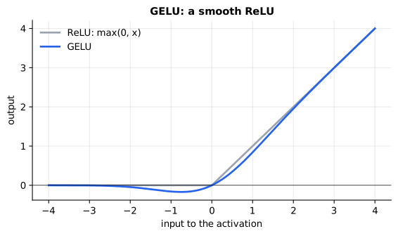
Reading it: the x-axis is the number going into the activation and the y-axis is what comes out. ReLU (grey) is a hard hinge: zero for every negative input, the identity for positives. GELU (blue) follows the same shape far from zero but bends smoothly around it and dips slightly below zero for small negatives. The smooth bend means the gradient never jumps, which is part of why transformers train well with it. (Many newer models use SwiGLU, a gated cousin of the same idea.)
Why it matters. Without a nonlinearity like GELU, the two matrix multiplies would collapse into one, and stacking layers would add nothing.
4. A tiny GPT, end to end
Everyday picture. An assembly line. Token ids go in one end, get turned into vectors, pass through a row of identical workstations (the blocks), get a final polish (the last norm), and come out the far end as a score for every word in the dictionary.
Tiny worked example. A model with a 50-token vocabulary, width 32, 2 blocks and 16 positions. The ids [3, 1, 4, 1, 5] become a 5 × 32 grid, pass through both blocks as 5 × 32, and come out as a 5 × 50 grid of logits (raw scores): row 5 scores every possible 6th token. It has 27,328 parameters.
flowchart LR
  IDS["ids [3,1,4,1,5]"] --> TE["token table lookup<br/>(50 × 32)"]
  POS["positions 0..4"] --> PE["position table lookup<br/>(16 × 32)"]
  TE --> ADD(("+"))
  PE --> ADD
  ADD --> B1["block 1"] --> B2["block 2"] --> LN["final layer norm"]
  LN --> OUT["× token tableᵀ<br/>logits (5 × 50)"]
  TE -. "same table (tied)" .- OUT
Reading it: the top-left path says what each token is, the bottom-left
path where it is (see primer.ml.positional); their sum enters the blocks.
Every block keeps the 5 × 32 shape. At the end, each token's final vector is
dot-producted with every row of the token table, giving one score per
vocabulary entry. The dotted line marks weight tying: the table that
turned ids into vectors on the way in is reused to score them on the way out,
saving vocab × width parameters.
The math and the code.
Level 3: the formula and its symbols
$$ \text{logits} = \text{LN}(h)\, E^{\top} $$
Symbols
| Symbol | Meaning here | In the example |
|---|---|---|
| $h$ | the vectors leaving the last block | 5 × 32 |
| $\text{LN}(h)$ | after the final layer norm | 5 × 32 |
| $E$ | the token embedding table, one row per vocabulary entry | 50 × 32 |
| $E^{\top}$ | $E$ transposed: rows become columns | 32 × 50 |
| logits | score of every vocabulary entry at every position | 5 × 50 |
In words: "score each candidate next token by how well its embedding lines up with the model's final vector."
With the numbers: row 5 of the logits holds 50 scores, one per token id;
softmax turns them into next-token probabilities (see
primer.ml.big_picture). TinyGPT.__call__ is this pipeline. Shrink it to
a width of 2 and a vocabulary of 3 to check by hand: a last position whose
normalized vector is LN(h) = (1, −1), against table rows (1, 0), (0, 1) and
(−1, 1), scores 1·1 + (−1)·0 = 1, then −1 and −2: token 0 lines
up best.
Level 3: in Python
In Python:
# LN(h) for the last position
ln_h = [1.0, -1.0]
# one row per vocabulary entry
E = [[1.0, 0.0], [0.0, 1.0], [-1.0, 1.0]]
# LN(h) Eᵀ: a dot product with each row
[sum(h_k * e_k for h_k, e_k in zip(ln_h, row)) for row in E]  # → [1.0, -1.0, -2.0]
In code: TinyGPT.hidden runs everything up to the final norm, and TinyGPT.n_params counts the 27,328 weights.
Why it matters. This is the whole forward pass of GPT-2, Llama and Claude-style models in miniature. Real models differ in size, not in kind.
5. Three families: encoder, decoder, encoder-decoder
Everyday picture. An editor reads the whole page before commenting on any sentence (encoder). A storyteller tells the story word by word and can't peek at words they haven't said yet (decoder). A translator reads the whole source sentence, then writes the translation word by word (encoder-decoder).
Tiny worked example. With 3 tokens, an encoder's attention may use all 9 (query, key) pairs; a decoder only the 6 on or below the diagonal. In the spec, changing token 5 changes token 1's output in an encoder block, and leaves it untouched in a decoder block.
flowchart TB
  subgraph ENC["Encoder-only (BERT)"]
    e1[every token sees every token] --> e2[a vector per token<br/>classify, embed, tag]
  end
  subgraph DEC["Decoder-only (GPT, Claude, Llama)"]
    d1[each token sees only the past] --> d2[predict the next token<br/>generate, chat, agents]
  end
  subgraph ED["Encoder-decoder (T5, original transformer)"]
    x1[encoder reads the source<br/>bidirectionally] --> x2[decoder writes the output causally,<br/>attending to the encoder too]
  end
Reading it: the three boxes differ only in who may attend to whom. The blocks inside are the same. That one choice of mask decides what the model is good at: seeing everything suits understanding tasks, and seeing only the past is what makes generation possible.
| Type | Example | Attention | Best for |
|---|---|---|---|
| Encoder-only | BERT | Bidirectional | Classification, embeddings, NER |
| Decoder-only | GPT, Claude, Llama | Causal | Generation, chat, agents |
| Encoder-decoder | T5, original transformer | Both | Translation, summarization |
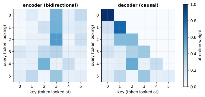
Reading it: both panels are attention weights from one block on the same 6 input vectors; rows are the token looking, columns the token looked at, darker is more weight. On the left (encoder) weight is spread over the whole grid. On the right (decoder) the upper-right triangle is empty, so nothing reads the future. Only the bottom row is identical in both panels: the last token sees everything either way, so the mask changes nothing for it. Every other decoder row differs, because its weights are shared out over only the tokens it may see: the first token, seeing only itself, puts all of its weight (1.0) there.
In code: TransformerBlock with its causal flag on is a decoder block and with it off an encoder block; mask_patterns runs one of each on the same input to draw the figure.
Why it matters. Embedding models (primer.ml.embeddings) are usually
encoders; chat models and agents are decoders.
6. Counting parameters
Everyday picture. Counting the bricks in a Lego model from its blueprint, without opening the box.
Tiny worked example. For width d, one block holds: attention 4·d² (W_q, W_k, W_v, W_o), feed-forward 8·d² (two d × 4d matrices), plus small bias and norm terms. With d = 32: 12 · 1,024 = 12,288, plus 160 (biases) plus 128 (norms) = 12,576 per block. Two blocks, plus tables of 50 × 32 and 16 × 32 and a final norm of 64, gives 27,328. The same recipe on GPT-2 small (d = 768, 12 blocks, 50,257 tokens, 1,024 positions) gives 124,402,944. GPT-2 also puts a bias on its attention projections, which the tiny model leaves out: 4·d = 3,072 more per block, 36,864 in all, and that brings it to exactly its published 124,439,808.
flowchart LR
  B["one block"] --> A["attention<br/>4·d²"]
  B --> F["feed-forward<br/>8·d²"]
  B --> N["norms and biases<br/>~13·d (tiny)"]
  A & F --> T["≈ 12·d² per block"]
  T --> ALL["× L blocks + embeddings<br/>vocab·d + positions·d"]
Reading it: almost all of a block's weight sits in two places, attention's four square matrices and the feed-forward's two wide ones. Everything else is a rounding error at large width, which is where the famous 12·L·d² rule comes from. Embeddings are added once, not per block.
The math.
Level 3: the formula and its symbols
$$ N \approx 12\, L\, d^2 + V d $$
Symbols
| Symbol | Meaning here | GPT-2 small |
|---|---|---|
| $N$ | total parameters | 124,439,808 |
| $L$ | number of blocks (layers) | 12 |
| $d$ | model width | 768 |
| $d^2$ | $d$ times $d$: the size of one square matrix | 589,824 |
| $V$ | vocabulary size | 50,257 |
| $Vd$ | the token embedding table | 38,597,376 |
In words: "about twelve square matrices per layer, plus the embedding table."
With the numbers: 12 · 12 · 589,824 = 84,934,656, plus 38,597,376 =
123,532,032, about 0.7% under the exact 124,439,808 (which also counts positions,
biases and norms; see gpt_param_count).
Level 3: in Python
In Python:
L, d, V = 12, 768, 50_257
# 12·L·d² and V·d
blocks, table = 12 * L * d ** 2, V * d
print(f"{blocks:,} + {table:,} = {blocks + table:,}")  # → 84,934,656 + 38,597,376 = 123,532,032
# the share it leaves out
round((124_439_808 - (blocks + table)) / 124_439_808, 3)  # → 0.007
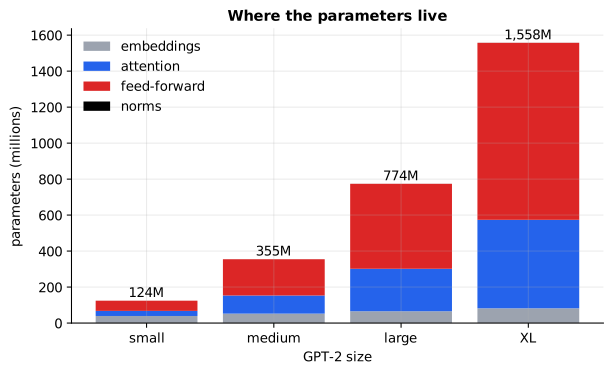
Reading it: each bar is one GPT-2 size, split by where the parameters live. Feed-forward (red) is always the largest block of the stack. In the small model, embeddings (grey) are almost a third of everything, because a 50k-row table is big next to 12 narrow layers. As models grow, the embeddings stay fixed while layers multiply, so their share shrinks to about 5% in XL, and the 12·L·d² term dominates.
In code: param_breakdown splits a GPT-2-shaped model's count into embeddings, attention, feed-forward and norms for the figure, and TransformerBlock.n_params counts one real block's weights.
Why it matters. Parameters × bytes per parameter is the memory a model
needs just to load (see primer.ml.inference for the arithmetic).
7. Mixture of Experts (MoE): a triage desk
Everyday picture. A hospital triage desk. Instead of one general practitioner seeing every patient, the desk sends each patient to the two most relevant specialists out of eight. The hospital employs eight doctors' worth of expertise, but each patient only takes up two doctors' time.
Tiny worked example. A router scores one token against 4 experts: (2.0, 1.0, 0.5, −1.0). Keep the top 2 (experts 0 and 1) and softmax just those two: e² / (e² + e¹) = 7.39 / 10.11 = 0.731, and 0.269. The token's output is 0.731 × expert 0's output + 0.269 × expert 1's output; experts 2 and 3 never run for this token.
flowchart LR
  X[token vector] --> R["router<br/>one score per expert"]
  R --> K["keep top 2<br/>softmax over them"]
  K -->|0.731| E0[expert 0: an FFN]
  K -->|0.269| E1[expert 1: an FFN]
  K -.->|skipped| E2[expert 2]
  K -.->|skipped| E3[expert 3]
  E0 --> S(("weighted sum"))
  E1 --> S
  S --> Y[output]
Reading it: the router is a tiny linear layer that scores the token against every expert. Only the two best-scoring experts run, and their outputs are blended by the renormalized scores (solid arrows); the others are skipped entirely (dotted). An MoE layer replaces the feed-forward network inside a block; attention is unchanged.
The math and the code.
Level 3: the formula and its symbols
$$ y = \sum_{i \in \text{TopK}(r)} g_i \, E_i(x), \qquad g = \text{softmax}\big(r_{\text{TopK}}\big), \qquad r = x W_r $$
Symbols
| Symbol | Meaning here | In the example |
|---|---|---|
| $x$ | one token's vector | |
| $W_r$ | the router's weights, width × number of experts | |
| $r$ | the router scores | (2.0, 1.0, 0.5, −1.0) |
| $\text{TopK}(r)$ | the positions of the $k$ largest scores | experts {0, 1} for k = 2 |
| $r_{\text{TopK}}$ | just those scores | (2.0, 1.0) |
| $g_i$ | expert $i$'s gate: softmax over the kept scores | 0.731, 0.269 |
| $E_i(x)$ | expert $i$ (a feed-forward network) applied to $x$ | |
| $\sum_{i \in \ldots}$ | add up over the chosen experts only | two terms |
In words: "score every expert, keep the best k, and blend those experts' outputs by their softmaxed scores."
With the numbers: y = 0.731 · E₀(x) + 0.269 · E₁(x). With 8 experts of
width 16, the layer holds 8 × 2,128 + 128 = 17,152 parameters, but one token
touches only 2 × 2,128 + 128 = 4,384. MixtureOfExperts and top_k_gates
are the code. Mixtral 8x7B works the same way: about 47B parameters in total,
about 13B active per token.
Level 3: in Python
In Python:
import math
r, k = [2.0, 1.0, 0.5, -1.0], 2
# TopK(r)
top_k = sorted(range(len(r)), key=lambda i: r[i], reverse=True)[:k]
top_k  # → [0, 1]
exps = [math.exp(r[i]) for i in top_k]
# g: softmax over the kept scores only
[round(e / sum(exps), 3) for e in exps]  # → [0.731, 0.269]
d, n_experts = 16, 8
# one expert is one feed-forward network
expert = d * 4 * d + 4 * d + 4 * d * d + d
# W_r
router = d * n_experts
# one, all held, touched per token
expert, n_experts * expert + router, k * expert + router  # → (2128, 17152, 4384)
A router left alone tends to play favourites, overloading some experts while others starve. Training adds a small load-balancing loss (Switch Transformer):
Level 3: the formula and its symbols
$$ \mathcal{L}_{\text{balance}} = n \sum_{i=1}^{n} f_i \, P_i $$
Symbols
| Symbol | Meaning here | Balanced example | Collapsed example |
|---|---|---|---|
| $n$ | number of experts | 4 | 4 |
| $f_i$ | share of routing slots that went to expert $i$ | ¼ each | (1, 0, 0, 0) |
| $P_i$ | expert $i$'s average router probability | ¼ each | ≈ (1, 0, 0, 0) |
| $\mathcal{L}$ | the penalty added to the training loss | 1.0 | ≈ 4.0 |
In words: "number of experts times the sum, over experts, of traffic share times average router probability."
With the numbers: balanced: 4 · (4 · ¼ · ¼) = 1.0, the minimum.
Collapsed onto one expert: 4 · (1 · 1) = 4.0, the maximum
(load_balancing_loss).
Level 3: in Python
In Python:
n = 4
def balance(f, P):
    # n Σ f_i P_i
    return n * sum(f_i * P_i for f_i, P_i in zip(f, P))
# every expert gets a quarter
balance([0.25] * n, [0.25] * n)  # → 1.0
# everything goes to expert 0
balance([1.0, 0.0, 0.0, 0.0], [1.0, 0.0, 0.0, 0.0])  # → 4.0
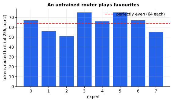
Reading it: each bar counts how many of 256 tokens an untrained router sent to each of 8 experts (top-2, so 512 slots in all); the dashed line is the perfectly even 64. Experts 3 and 5 get 75 tokens each while expert 2 gets only 51: even random routing is lopsided, and in training the imbalance compounds because favoured experts improve and attract more traffic. The balancing loss pushes the bars back towards the line.
In code: MixtureOfExperts.n_params and MixtureOfExperts.active_params give the 17,152 and 4,384 above, and MixtureOfExperts.tokens_per_expert counts the bars in the figure.
Why it matters. MoE lets a model hold far more knowledge (parameters) for the same compute per token, which is why many frontier models use it. The price is memory: every expert must be loaded even though few run per token.
8. Compute arithmetic: 2N to generate, 6N to train
Everyday picture. Every parameter does one multiply and one add for every token that passes through it, like a toll booth that charges two coins per car.
Tiny worked example. A 7B-parameter model generating one token: 2 × 7e9 = 1.4e10 operations (14 GFLOPs). Training a 70B model on a trillion tokens: 6 × 70e9 × 1e12 = 4.2e23 operations.
flowchart LR
  F["forward pass<br/>2 FLOPs per parameter per token"] --> L[loss]
  L --> B["backward pass<br/>≈ 4 FLOPs per parameter per token"]
  B --> T["training total ≈ 6·N per token"]
  F --> I["inference total ≈ 2·N per token"]
Reading it: inference only runs the forward pass, so it pays 2 per
parameter per token. Training runs the same forward pass, then a backward
pass (primer.ml.neural_net) that costs about twice as much, because it
computes gradients both for the weights and for the activations. 2 + 4 = 6.
The math.
Level 3: the formula and its symbols
$$ C_{\text{infer}} \approx 2N \text{ per token}, \qquad C_{\text{train}} \approx 6ND $$
Symbols
| Symbol | Meaning here | In the example |
|---|---|---|
| $N$ | number of parameters | 7e9 / 70e9 / 175e9 |
| $D$ | number of training tokens | 1e12 / 300e9 |
| $C$ | compute in FLOPs (floating-point operations: one multiply or one add) | |
| $e$ in 7e9 | "times 10 to the power": 7e9 = 7,000,000,000 |
In words: "generating costs two operations per parameter per token; training costs six per parameter per training token."
With the numbers: GPT-3: 6 × 175e9 × 300e9 = 3.15e23 FLOPs, matching
the roughly 3.14e23 its paper reports (training_flops,
inference_flops_per_token).
Level 3: in Python
In Python:
def C_infer(N):
    # per generated token
    return 2 * N
def C_train(N, D):
    # over all D training tokens
    return 6 * N * D
print(f"{C_infer(7e9):.2g}  {C_train(70e9, 1e12):.2g}  {C_train(175e9, 300e9):.3g}")  # → 1.4e+10 4.2e+23 3.15e+23
Why it matters. These two lines let you estimate GPU-hours, serving cost and training budgets on the back of an envelope.
In 20 seconds
- A block is attention (tokens exchange information) then a feed-forward network (each token processes alone), each wrapped in a residual add and a layer norm (pre-norm).
- A GPT is: embed tokens and positions, run N blocks, normalize, and score every vocabulary entry with the (tied) embedding table.
- Parameters ≈ 12·L·d² + vocab·d; compute ≈ 2N per generated token and 6ND to train. MoE adds experts to grow parameters without growing per-token compute.
Self-test questions
What do attention and the feed-forward network each contribute? Attention mixes information across tokens; the feed-forward network transforms each token independently and holds most of the parameters (and, it's thought, much of the factual knowledge).
Why residual connections? Each sub-layer adds a correction instead of replacing its input, so signal and gradients have a direct path through very deep stacks.
Pre-norm vs. post-norm? Pre-norm normalizes before each sub-layer and leaves the residual path untouched; it trains more stably, so modern models use it.
Why LayerNorm rather than BatchNorm in transformers? It normalizes within each token, so it doesn't depend on batch size or sequence length.
Roughly how many parameters does a model with 32 layers of width 4096 have, not counting embeddings? 12 · 32 · 4096² ≈ 6.4 billion.
Encoder-only vs. decoder-only? Encoders attend bidirectionally and suit classification and embeddings; decoders attend causally and generate text.
What does Mixture of Experts buy you, and what does it cost? More total parameters at the same compute per token, since each token runs only k experts. It costs memory (all experts loaded), routing complexity and load-balancing.
Estimate the compute to train a 7B model on 2 trillion tokens. 6 × 7e9 × 2e12 = 8.4e22 FLOPs.
The papers behind this lesson
- Vaswani et al. (2017), Attention Is All You Need. https://arxiv.org/abs/1706.03762. Introduced the transformer block: attention plus feed-forward, residuals and layer norm, stacked. annotated companion
- Ba, Kiros & Hinton (2016), Layer Normalization. https://arxiv.org/abs/1607.06450. Normalized within each example instead of across the batch, the variant transformers use. annotated companion
- Zhang & Sennrich (2019), Root Mean Square Layer Normalization. https://arxiv.org/abs/1910.07467. Dropped the mean-centring for a cheaper norm now used by most LLMs.
- Hendrycks & Gimpel (2016), Gaussian Error Linear Units (GELUs). https://arxiv.org/abs/1606.08415. The smooth activation used in GPT-2 and BERT.
- Xiong et al. (2020), On Layer Normalization in the Transformer Architecture. https://arxiv.org/abs/2002.04745. Explained why pre-norm trains more stably than post-norm.
- Devlin et al. (2018), BERT. https://arxiv.org/abs/1810.04805. The canonical encoder-only model.
- Fedus, Zoph & Shazeer (2021), Switch Transformers. https://arxiv.org/abs/2101.03961. Scaled Mixture of Experts and introduced the load-balancing loss built here.
- Jiang et al. (2024), Mixtral of Experts. https://arxiv.org/abs/2401.04088. An open top-2-of-8 MoE model: about 47B parameters, about 13B active per token.
- Kaplan et al. (2020), Scaling Laws for Neural Language Models. https://arxiv.org/abs/2001.08361. Popularized the 6·N·D compute estimate. annotated companion
Further reading
- The Annotated Transformer (Harvard NLP): https://nlp.seas.harvard.edu/annotated-transformer/
- The Illustrated Transformer (Jay Alammar): https://jalammar.github.io/illustrated-transformer/
- Andrej Karpathy, Let's build GPT (video): https://www.youtube.com/watch?v=kCc8FmEb1nY
- Karpathy's
nanoGPT: https://github.com/karpathy/nanoGPT - Hugging Face LLM course, How do Transformers work?: https://huggingface.co/learn/llm-course/chapter1/4
- Hugging Face blog, Mixture of Experts Explained: https://huggingface.co/blog/moe
1r""" 2# The transformer block: the unit every modern LLM stacks 3 4Run: `python -m primer.ml.transformer` 5 6New to the notation (vectors, matrix multiply, mean, square root)? Every 7symbol is decoded where it appears, and `primer.notation` teaches them all 8from zero. This lesson builds on `primer.ml.attention`. 9 10Read alongside the annotated paper: [Attention Is All You Need, annotated](../../papers/attention-is-all-you-need.html). 11 12## Level 1: The practitioner's guide 13 14**In one sentence.** The transformer block (attention, then a feed-forward 15network that works on each token alone, each wrapped in a residual add and 16a normalization) is the unit every modern language model stacks, and 17reading a model's block count, width and expert layout off its card tells 18you its memory, its speed and its training cost before you download it. 19 20**When you need it.** You never build a block; you meet its numbers. The 21day comes when you choose between a dense 70B model and one that calls 22itself "8x7B", size a GPU for a download, estimate what a fine-tune or a 23pretraining run will cost, pick an encoder or a decoder for an embedding or 24classification job, or open a `config.json` and need to turn 25`num_hidden_layers`, `hidden_size`, `intermediate_size` and 26`num_local_experts` into gigabytes and dollars. The rule of thumb behind all 27of it, from this lesson's `gpt_param_count`: parameters are about twelve 28square matrices per block plus the embedding table, 12 · L · d² + V · d. For 29GPT-2 small that gives 123,532,032, within 0.7% of the exact 124,439,808. 30When you call a hosted model by name, the vendor has already made these 31choices; the block then matters only as the reason you pay per token, and 32you can skip to the cost section. 33 34**Your options.** The choices below are the ones a practitioner makes 35around the block: which family, dense or sparse, and how a parameter count 36becomes hardware. From the plainest to the most involved: 37 38| Option | What it does | What it gives you | What it costs | Where it lives | 39|---|---|---|---|---| 40| Encoder-only (BERT) | Every token attends to every token, both directions | One vector per token: classification, embeddings, tagging | Cannot generate; a fixed maximum length | Embedding and classifier models | 41| Encoder-decoder (T5, the 2017 transformer) | An encoder reads the source; a decoder writes the output while attending to it | Translation and summarization with a clean split between reading and writing | Two stacks to train and serve; rarely used for chat | Sequence-to-sequence models | 42| Decoder-only, dense (GPT, Llama, Claude) | Each token sees only the past; every block's feed-forward network runs for every token | Generation, chat, agents; the simplest to serve | About 2N operations per generated token, and all N parameters in memory | The model family you pick | 43| Decoder-only, mixture of experts (Mixtral, DeepSeek-V3) | Each block routes each token to k of E expert feed-forward networks | Far more parameters per unit of compute: Mixtral 8x7B holds about 47B and runs about 13B per token; DeepSeek-V3 holds 671B and runs 37B | Every expert must be loaded, so memory for all E and compute for k; a router and a balancing loss to keep experts busy | The model family; `num_local_experts`, `num_experts_per_tok` | 44| A smaller model trained longer | The vendor picks N below the compute-optimal size and trains far past 20 tokens per parameter | A model that is cheaper to serve forever: Llama 3 8B saw more than 15 trillion tokens | More training compute up front, paid once by the vendor | The card's training-token count | 45| Quantization at load time | Stores each parameter in fewer bits | A 70B model at 4 bits is 35 GB instead of 140 GB and fits one 80 GB GPU | Some quality loss, measured per model (`primer.ml.inference`) | The serving stack | 46 47**How to choose.** Start from the job, then the hardware. 48 49- Generating text, chatting, calling tools: a decoder. Embeddings, 50 classification, tagging: an encoder, or a decoder's final vectors 51 (`primer.ml.embeddings`). 52- Dense or mixture of experts for a model you host: experts win when memory 53 is plentiful and compute per token is the constraint (many concurrent 54 users); dense wins when memory is tight, because Mixtral's 47B parameters 55 must all be resident (about 94 GB at 16 bits) to run its 13B. 56- Sizing memory: parameters times bytes per parameter. 70B at 16 bits is 57 140 GB, more than one 80 GB GPU; at 4 bits it is 35 GB. 58- Estimating a training run: 6 · N · D. A 7B model on its compute-optimal 59 140 billion tokens costs 5.88 × 10²¹ operations, about 4,100 GPU-hours at 60 a sustained 400 teraFLOP/s per GPU (`primer.ml.pretraining`). 61- Reading a config: blocks L, width d, feed-forward width (14,336 against 62 4,096 for Llama 3 8B, about 3.5×), vocabulary V, and the expert counts. 63 With those you can reproduce the parameter count before downloading. 64- Whatever you pick, remember that the block is the same in all of them. 65 The differences of kind are the attention mask and whether the 66 feed-forward network is routed; everything else is size. 67 68**What it costs.** Three currencies: memory, compute and, for experts, the 69gap between the two. 70 71- Memory. Parameters × bytes. GPT-2 ran from 124 million (12 blocks, width 72 768) to 1.56 billion (48 blocks, width 1,600); Llama 3 runs from 8B (32 73 blocks, width 4,096) through 70B (80 blocks, width 8,192) to 405B (126 74 blocks, width 16,384), each with 8 key-value heads. The feed-forward 75 network is always the largest share, and the embedding table shrinks from 76 32% of GPT-2 small to 5% of XL as blocks multiply (`param_breakdown`). 77- Compute. About 2N operations per generated token (a 7B model: 1.4 × 10¹⁰, 78 14 GFLOPs) and about 6 · N · D to train (GPT-3: 3.15 × 10²³, matching the 79 paper's 3.14 × 10²³). Llama 3 405B took 3.8 × 10²⁵ operations over 15.6 80 trillion tokens on up to 16,000 H100 GPUs, and DeepSeek-V3 reports 2.788 81 million H800 GPU-hours over 14.8 trillion tokens. 82- Experts. This lesson's 8 experts of width 16 hold 17,152 parameters while 83 one token touches 4,384: the whole point, and the whole catch. You buy 84 knowledge with memory and pay compute only for what each token uses. 85 86**What breaks.** 87 88- **Reading "8x7B" as 56B or as 7B.** It is neither: about 47B to load, 89 because only the feed-forward networks are multiplied by eight (attention 90 and embeddings are not), and about 13B to run per token. Size the GPU for the first number and the latency for the 91 second. 92- **Experts that starve.** Even an untrained router is lopsided: in this 93 lesson's run experts 3 and 5 receive 75 of 256 tokens each while expert 2 94 receives 51, and in training the imbalance compounds because busy experts 95 improve and attract more traffic. The balancing loss is the fix; Hugging 96 Face's Mixtral config keeps it on with `router_aux_loss_coef` at 0.001. 97 Leave it on when you fine-tune an expert model. 98- **Normalizing after instead of before.** The 2017 layout put the norm 99 after each sub-layer; pre-norm, with the norm before and the residual 100 path untouched, trains more stably (Xiong et al., 2020) and is what modern 101 models use. If you assemble blocks yourself, copy the modern order. 102- **A stack with no skip path.** Replace the residual add with plain 103 replacement and a hundred blocks cannot train; the spec checks that a 104 block with both sub-layers switched off returns its input unchanged. 105- **The wrong mask for the job.** An encoder cannot generate, and a 106 decoder's per-token vectors only ever saw the past, which is why 107 embedding models are usually encoders. 108- **Forgetting the embedding table.** For a small model it is not a 109 rounding error: 38.6 million of GPT-2 small's 124 million parameters, 32% 110 of the total. 111 112**In the wild.** GPT-2 ships in the four sizes counted above, and this 113lesson's count lands on its exact 124,439,808 once the attention biases are 114included. Llama 3's herd (8B, 70B, 405B) uses RMSNorm, SwiGLU feed-forward 115networks and grouped-query attention inside the same block. Mixtral 8x7B 116and DeepSeek-V3 are the reference mixture-of-experts models, and the Switch 117Transformer paper (Fedus, Zoph and Shazeer, 2021) introduced the balancing 118loss built here. Hugging Face configs name the block's numbers directly: 119`num_hidden_layers`, `hidden_size`, `intermediate_size`, 120`num_attention_heads`, `num_key_value_heads`, `vocab_size` and, for 121experts, `num_local_experts` and `num_experts_per_tok`. The 6 · N · D rule 122comes from Kaplan et al. (2020) and the 20-tokens-per-parameter rule from 123Hoffmann et al. (2022). BERT is the canonical encoder and T5 the canonical 124encoder-decoder. The papers are linked at the end of the lesson. 125 126**Go deeper.** Level 2 builds a block on a two-number token, normalizes 127(1, 2, 3, 4) by hand, runs one number through GELU, assembles a 27,328-parameter 128GPT, draws the three families' masks, counts GPT-2 to the exact parameter, 129routes a token through a mixture of experts with its balancing loss, and 130derives the 2N and 6N rules. If you only needed to read a model card or 131size a machine, you are done. 132 133## Level 2: How it works, from scratch 134 135Level 2 assembles the block one piece at a time, starting with the picture 136of a team that meets, then works alone. 137 138## 1. The block: a meeting, then desk work 139 140**Everyday picture.** A team works in rounds. Each round starts with a 141**meeting**, where everyone listens to everyone else and takes notes on what's 142relevant to them (that's attention). Then comes **desk work**: each person 143goes back to their own desk and thinks through their notes alone, without 144talking to anyone (that's the feed-forward network). Nobody throws away their 145old notes; they only add to them (the *residual connection*). A large model 146runs dozens of these rounds: GPT-2 small has 12, big models have 80 or more. 147 148**Tiny worked example.** Take one token whose vector is x = (1, 2). The 149meeting produces a correction (0.1, −0.3); adding it gives (1.1, 1.7). Desk 150work then adds (−0.2, 0.4), giving (0.9, 2.1). The token's vector has been 151*edited twice*, never replaced. 152 153```mermaid 154flowchart TD 155 IN[Input vectors<br/>one per token] --> N1[Layer norm] 156 N1 --> AT[Multi-head attention<br/>the meeting: mix across tokens] 157 AT --> R1((Add)) 158 IN --> R1 159 R1 --> N2[Layer norm] 160 N2 --> FF[Feed-forward network<br/>desk work: each token alone] 161 FF --> R2((Add)) 162 R1 --> R2 163 R2 --> OUT[To the next block] 164``` 165 166**Reading it:** follow the main line straight down the left. The input is 167first normalized (rescaled, section 2) and fed to attention. Attention's 168output does *not* replace the input: the "Add" circle adds it to the original, 169which arrives by the side arrow that skips the whole step. The same pattern 170repeats for the feed-forward network. Those two skip arrows are the 171**residual connections**. Because every step only adds a correction, the 172signal (and during training, the gradient) has an unobstructed highway 173through a hundred blocks. This layout, with the norm *before* each sub-layer, 174is called **pre-norm**; it trains more stably than the 2017 original, which 175normalized after. 176 177**The math and the code.** 178 179$$ 180x \leftarrow x + \text{Attn}(\text{LN}(x)), \qquad x \leftarrow x + \text{FFN}(\text{LN}(x)) 181$$ 182 183**Symbols** 184 185| Symbol | Meaning here | In the example | 186|---|---|---| 187| $x$ | the token vectors, one row per token (the "residual stream") | (1, 2) for one token | 188| $\leftarrow$ | "replace the left side with the right side", as in code: `x = x + ...` | | 189| $\text{LN}(\cdot)$ | layer normalization (section 2) | | 190| $\text{Attn}(\cdot)$ | multi-head attention from `primer.ml.attention`: the meeting | returns (0.1, −0.3) | 191| $\text{FFN}(\cdot)$ | the feed-forward network (section 3): desk work | returns (−0.2, 0.4) | 192| $+$ | add the correction to the vector, number by number | | 193 194**In words:** "add what the meeting found to each token's notes, then add 195what each token worked out alone." 196 197**With the numbers:** (1, 2) + (0.1, −0.3) = (1.1, 1.7); then (1.1, 1.7) + 198(−0.2, 0.4) = **(0.9, 2.1)**. `TransformerBlock.__call__` is exactly these 199two lines. 200 201**In Python:** 202 203```python 204x = [1.0, 2.0] 205# what Attn(LN(x)) returned 206attn = [0.1, -0.3] 207# x ← x + Attn(LN(x)) 208x = [x_j + a_j for x_j, a_j in zip(x, attn)] 209[round(x_j, 1) for x_j in x] # → [1.1, 1.7] 210# what FFN(LN(x)) returned 211ffn = [-0.2, 0.4] 212# x ← x + FFN(LN(x)) 213x = [x_j + f_j for x_j, f_j in zip(x, ffn)] 214[round(x_j, 1) for x_j in x] # → [0.9, 2.1] 215``` 216 217**In code:** `TransformerBlock` holds one `primer.ml.attention.MultiHeadAttention`, one `FeedForward` and the two norms' learned gains and biases. 218 219**Why it matters.** The block's output has the same shape as its input, so 220blocks stack like Lego. And because the input is never overwritten, switching 221both sub-layers off gives back the input unchanged (a scenario in the spec), 222which is why very deep stacks train at all. 223 224## 2. Layer normalization: grading each token on its own curve 225 226**Everyday picture.** A teacher grading on a curve: subtract the class 227average from each score, then divide by how spread out the scores are. After 228that, "2 above average" means the same thing in every class. LayerNorm does 229this to the numbers *inside one token's vector*, so no token's numbers can 230drift huge or tiny as they pass through dozens of blocks. 231 232**Tiny worked example.** Normalize (1, 2, 3, 4). The **mean** (average) is 2332.5. The **variance** (average squared distance from the mean) is 234(2.25 + 0.25 + 0.25 + 2.25) / 4 = 1.25, so the spread (**standard 235deviation**, its square root) is 1.118. Result: (−1.342, −0.447, 0.447, 2361.342). Multiply the input by 100 and the result is identical. 237 238```mermaid 239flowchart LR 240 X["one token: (1, 2, 3, 4)"] --> M["subtract the mean 2.5<br/>(−1.5, −0.5, 0.5, 1.5)"] 241 M --> S["divide by the spread 1.118<br/>(−1.342, −0.447, 0.447, 1.342)"] 242 S --> G["× learned gain, + learned bias<br/>(start as 1 and 0)"] 243``` 244 245**Reading it:** two fixed steps, then one learned step. Centring and 246dividing force every token's numbers to average 0 with spread 1; the learned 247gain and bias then let the model pick whatever scale each feature actually 248needs. RMSNorm (used by Llama and most recent models) skips the centring box 249and divides by the root-mean-square instead: cheaper, and it works as well. 250 251**The math and the code.** 252 253$$ 254\text{LN}(x)_j = \gamma_j \,\frac{x_j - \mu}{\sqrt{\sigma^2 + \epsilon}} + \beta_j, 255\qquad \mu = \frac{1}{d}\sum_{j=1}^{d} x_j, \qquad \sigma^2 = \frac{1}{d}\sum_{j=1}^{d}(x_j - \mu)^2 256$$ 257 258**Symbols** 259 260| Symbol | Meaning here | In the example | 261|---|---|---| 262| $x$ | one token's vector | (1, 2, 3, 4) | 263| $d$ | how many numbers it has | 4 | 264| $j$ | a counter over those numbers, 1 to $d$ | | 265| $x_j$ | the $j$-th number | $x_1 = 1$ | 266| $\sum_{j=1}^{d}$ | "add up the following for $j$ = 1, 2, ..., $d$" | | 267| $\mu$ (mu) | the mean | 2.5 | 268| $\sigma^2$ (sigma squared) | the variance | 1.25 | 269| $\sqrt{\cdot}$ | square root; $\sqrt{\sigma^2}$ is the spread | 1.118 | 270| $\epsilon$ (epsilon) | a tiny number (1e-5) so we never divide by zero | 0.00001 | 271| $\gamma_j, \beta_j$ (gamma, beta) | learned gain and bias per feature | 1 and 0 at the start | 272 273**In words:** "subtract the token's average from each of its numbers, divide 274by the token's spread, then rescale and shift each feature by learned 275amounts." 276 277**With the numbers:** $x_1$: (1 − 2.5) / √(1.25 + 0.00001) = −1.5 / 1.118 = 278**−1.342**, then × 1 + 0 = −1.342. `layer_norm` and `rms_norm` implement 279both variants. 280 281**In Python:** 282 283```python 284import math 285x = [1, 2, 3, 4] 286d = len(x) 287# μ = (1/d) Σ x_j 288mu = sum(x) / d 289# σ² = (1/d) Σ (x_j − μ)² 290sigma2 = sum((x_j - mu) ** 2 for x_j in x) / d 291mu, sigma2 # → (2.5, 1.25) 292# learned gain and bias start at 1 and 0 293eps, gamma, beta = 1e-5, 1.0, 0.0 294[round(gamma * (x_j - mu) / math.sqrt(sigma2 + eps) + beta, 3) for x_j in x] # → [-1.342, -0.447, 0.447, 1.342] 295``` 296 297**Why it matters.** Without normalization, activations drift layer after 298layer until training blows up or stalls. It normalizes per token (not per 299batch, unlike the BatchNorm used in image networks), so it works for any 300batch size and sequence length. 301 302## 3. The feed-forward network: desk work 303 304**Everyday picture.** Back at their desk, each person spreads their notes 305out over a desk four times wider than the notebook, underlines what matters, 306and writes a short summary back into the notebook. Nobody talks to anyone. 307 308**Tiny worked example.** With model width 8, the network widens each token 309to 32 numbers, applies GELU to each, and narrows back to 8. Parameters: 3108·32 + 32 + 32·8 + 8 = **552**. GELU on single numbers: GELU(1) = 0.841, 311GELU(10) = 10.0, GELU(−3) = −0.004, GELU(0) = 0. 312 313```mermaid 314flowchart LR 315 X["token vector<br/>d numbers"] --> W1["× W1 + b1<br/>widen to 4·d"] 316 W1 --> G["GELU on each number<br/>keep positives, squash negatives"] 317 G --> W2["× W2 + b2<br/>back to d"] 318 W2 --> Y["correction for this token"] 319``` 320 321**Reading it:** a token's vector goes in on the left, alone. It is widened 322by a matrix multiply, passed through a smooth on/off switch (GELU) number by 323number, and narrowed back. The same weights are applied to every token 324separately, so this step never mixes tokens; it transforms each one using 325what attention already gathered. Two thirds of each block's parameters 326live here (8d² of every 12d²); counting the embedding table too, that is 45% 327of GPT-2 small and 63% of GPT-2 XL (chapter 6). Much of a model's factual 328knowledge is thought to be stored in these weights. 329 330**The math and the code.** A **matrix multiply** $xW$ turns a list of $d$ 331numbers into a list of $4d$ numbers: each output number is the dot product of 332$x$ with one column of $W$ (multiply matching numbers, add them up). 333 334$$ 335\text{FFN}(x) = \text{GELU}(x W_1 + b_1)\, W_2 + b_2, 336\qquad \text{GELU}(z) \approx \tfrac{1}{2} z \left(1 + \tanh\!\left(\sqrt{2/\pi}\,(z + 0.044715\, z^3)\right)\right) 337$$ 338 339**Symbols** 340 341| Symbol | Meaning here | In the example | 342|---|---|---| 343| $x$ | one token's vector | 8 numbers | 344| $W_1$ | first weight matrix, widens | 8 × 32 | 345| $b_1$ | first bias, added after widening | 32 numbers | 346| $W_2$ | second weight matrix, narrows | 32 × 8 | 347| $b_2$ | second bias | 8 numbers | 348| $z$ | any single number fed to GELU | 1 | 349| $\tanh$ | "hyperbolic tangent": an S-shaped curve from −1 to +1 | $\tanh(0.8)$ = 0.664 | 350| $\pi$ | pi, 3.14159... | | 351| $\approx$ | "approximately equals": this tanh form is a fast stand-in for exact GELU | | 352 353**In words:** "widen the token with a matrix multiply, softly switch off 354negative numbers, then narrow it back with another matrix multiply." 355 356**With the numbers:** GELU(1) = ½ · 1 · (1 + tanh(0.798 · 1.045)) = ½ · (1 + 357tanh(0.834)) = ½ · (1 + 0.683) = **0.841**. `FeedForward` and `gelu` are the 358code. 359 360**In Python:** 361 362```python 363import math 364def gelu(z): 365 return 0.5 * z * (1 + math.tanh(math.sqrt(2 / math.pi) * (z + 0.044715 * z ** 3))) 366[round(gelu(z), 3) for z in (1, 10, -3, 0)] # → [0.841, 10.0, -0.004, 0.0] 367d = 8 368# W1 (8 × 32), b1, W2 (32 × 8), b2 369d * 4 * d + 4 * d + 4 * d * d + d # → 552 370``` 371 372 373 374**Reading it:** the x-axis is the number going into the activation and the 375y-axis is what comes out. ReLU (grey) is a hard hinge: zero for every 376negative input, the identity for positives. GELU (blue) follows the same 377shape far from zero but bends smoothly around it and dips slightly below 378zero for small negatives. The smooth bend means the gradient never jumps, 379which is part of why transformers train well with it. (Many newer models use 380SwiGLU, a gated cousin of the same idea.) 381 382**Why it matters.** Without a nonlinearity like GELU, the two matrix 383multiplies would collapse into one, and stacking layers would add nothing. 384 385## 4. A tiny GPT, end to end 386 387**Everyday picture.** An assembly line. Token ids go in one end, get turned 388into vectors, pass through a row of identical workstations (the blocks), get 389a final polish (the last norm), and come out the far end as a score for every 390word in the dictionary. 391 392**Tiny worked example.** A model with a 50-token vocabulary, width 32, 2 393blocks and 16 positions. The ids [3, 1, 4, 1, 5] become a 5 × 32 grid, pass 394through both blocks as 5 × 32, and come out as a 5 × 50 grid of **logits** 395(raw scores): row 5 scores every possible 6th token. It has **27,328** 396parameters. 397 398```mermaid 399flowchart LR 400 IDS["ids [3,1,4,1,5]"] --> TE["token table lookup<br/>(50 × 32)"] 401 POS["positions 0..4"] --> PE["position table lookup<br/>(16 × 32)"] 402 TE --> ADD(("+")) 403 PE --> ADD 404 ADD --> B1["block 1"] --> B2["block 2"] --> LN["final layer norm"] 405 LN --> OUT["× token tableᵀ<br/>logits (5 × 50)"] 406 TE -. "same table (tied)" .- OUT 407``` 408 409**Reading it:** the top-left path says *what* each token is, the bottom-left 410path *where* it is (see `primer.ml.positional`); their sum enters the blocks. 411Every block keeps the 5 × 32 shape. At the end, each token's final vector is 412dot-producted with every row of the token table, giving one score per 413vocabulary entry. The dotted line marks **weight tying**: the table that 414turned ids into vectors on the way in is reused to score them on the way out, 415saving vocab × width parameters. 416 417**The math and the code.** 418 419$$ 420\text{logits} = \text{LN}(h)\, E^{\top} 421$$ 422 423**Symbols** 424 425| Symbol | Meaning here | In the example | 426|---|---|---| 427| $h$ | the vectors leaving the last block | 5 × 32 | 428| $\text{LN}(h)$ | after the final layer norm | 5 × 32 | 429| $E$ | the token embedding table, one row per vocabulary entry | 50 × 32 | 430| $E^{\top}$ | $E$ **transposed**: rows become columns | 32 × 50 | 431| logits | score of every vocabulary entry at every position | 5 × 50 | 432 433**In words:** "score each candidate next token by how well its embedding 434lines up with the model's final vector." 435 436**With the numbers:** row 5 of the logits holds 50 scores, one per token id; 437softmax turns them into next-token probabilities (see 438`primer.ml.big_picture`). `TinyGPT.__call__` is this pipeline. Shrink it to 439a width of 2 and a vocabulary of 3 to check by hand: a last position whose 440normalized vector is LN(h) = (1, −1), against table rows (1, 0), (0, 1) and 441(−1, 1), scores 1·1 + (−1)·0 = **1**, then **−1** and **−2**: token 0 lines 442up best. 443 444**In Python:** 445 446```python 447# LN(h) for the last position 448ln_h = [1.0, -1.0] 449# one row per vocabulary entry 450E = [[1.0, 0.0], [0.0, 1.0], [-1.0, 1.0]] 451# LN(h) Eᵀ: a dot product with each row 452[sum(h_k * e_k for h_k, e_k in zip(ln_h, row)) for row in E] # → [1.0, -1.0, -2.0] 453``` 454 455**In code:** `TinyGPT.hidden` runs everything up to the final norm, and `TinyGPT.n_params` counts the 27,328 weights. 456 457**Why it matters.** This is the whole forward pass of GPT-2, Llama and 458Claude-style models in miniature. Real models differ in size, not in kind. 459 460## 5. Three families: encoder, decoder, encoder-decoder 461 462**Everyday picture.** An **editor** reads the whole page before commenting 463on any sentence (encoder). A **storyteller** tells the story word by word 464and can't peek at words they haven't said yet (decoder). A **translator** 465reads the whole source sentence, then writes the translation word by word 466(encoder-decoder). 467 468**Tiny worked example.** With 3 tokens, an encoder's attention may use all 9 469(query, key) pairs; a decoder only the 6 on or below the diagonal. In the 470spec, changing token 5 changes token 1's output in an encoder block, and 471leaves it untouched in a decoder block. 472 473```mermaid 474flowchart TB 475 subgraph ENC["Encoder-only (BERT)"] 476 e1[every token sees every token] --> e2[a vector per token<br/>classify, embed, tag] 477 end 478 subgraph DEC["Decoder-only (GPT, Claude, Llama)"] 479 d1[each token sees only the past] --> d2[predict the next token<br/>generate, chat, agents] 480 end 481 subgraph ED["Encoder-decoder (T5, original transformer)"] 482 x1[encoder reads the source<br/>bidirectionally] --> x2[decoder writes the output causally,<br/>attending to the encoder too] 483 end 484``` 485 486**Reading it:** the three boxes differ only in *who may attend to whom*. 487The blocks inside are the same. That one choice of mask decides what the 488model is good at: seeing everything suits understanding tasks, and seeing 489only the past is what makes generation possible. 490 491| Type | Example | Attention | Best for | 492|-----------------|--------------------------|---------------|---------------------------------| 493| Encoder-only | BERT | Bidirectional | Classification, embeddings, NER | 494| Decoder-only | GPT, Claude, Llama | Causal | Generation, chat, agents | 495| Encoder-decoder | T5, original transformer | Both | Translation, summarization | 496 497 498 499**Reading it:** both panels are attention weights from one block on the 500same 6 input vectors; rows are the token looking, columns the token looked 501at, darker is more weight. On the left (encoder) weight is spread over the 502whole grid. On the right (decoder) the upper-right triangle is empty, so 503nothing reads the future. Only the bottom row is identical in both panels: 504the last token sees everything either way, so the mask changes nothing for 505it. Every other decoder row differs, because its weights are shared out over 506only the tokens it may see: the first token, seeing only itself, puts all 507of its weight (1.0) there. 508 509**In code:** `TransformerBlock` with its causal flag on is a decoder block and with it off an encoder block; `mask_patterns` runs one of each on the same input to draw the figure. 510 511**Why it matters.** Embedding models (`primer.ml.embeddings`) are usually 512encoders; chat models and agents are decoders. 513 514## 6. Counting parameters 515 516**Everyday picture.** Counting the bricks in a Lego model from its 517blueprint, without opening the box. 518 519**Tiny worked example.** For width d, one block holds: attention 4·d² 520(W_q, W_k, W_v, W_o), feed-forward 8·d² (two d × 4d matrices), plus small 521bias and norm terms. With d = 32: 12 · 1,024 = 12,288, plus 160 (biases) plus 522128 (norms) = 12,576 per block. Two blocks, plus tables of 50 × 32 and 16 × 32 523and a final norm of 64, gives **27,328**. The same recipe on GPT-2 small 524(d = 768, 12 blocks, 50,257 tokens, 1,024 positions) gives 124,402,944. 525GPT-2 also puts a bias on its attention projections, which the tiny model 526leaves out: 4·d = 3,072 more per block, 36,864 in all, and that brings it to 527exactly its published **124,439,808**. 528 529```mermaid 530flowchart LR 531 B["one block"] --> A["attention<br/>4·d²"] 532 B --> F["feed-forward<br/>8·d²"] 533 B --> N["norms and biases<br/>~13·d (tiny)"] 534 A & F --> T["≈ 12·d² per block"] 535 T --> ALL["× L blocks + embeddings<br/>vocab·d + positions·d"] 536``` 537 538**Reading it:** almost all of a block's weight sits in two places, 539attention's four square matrices and the feed-forward's two wide ones. 540Everything else is a rounding error at large width, which is where the 541famous 12·L·d² rule comes from. Embeddings are added once, not per block. 542 543**The math.** 544 545$$ 546N \approx 12\, L\, d^2 + V d 547$$ 548 549**Symbols** 550 551| Symbol | Meaning here | GPT-2 small | 552|---|---|---| 553| $N$ | total parameters | 124,439,808 | 554| $L$ | number of blocks (layers) | 12 | 555| $d$ | model width | 768 | 556| $d^2$ | $d$ times $d$: the size of one square matrix | 589,824 | 557| $V$ | vocabulary size | 50,257 | 558| $Vd$ | the token embedding table | 38,597,376 | 559 560**In words:** "about twelve square matrices per layer, plus the embedding 561table." 562 563**With the numbers:** 12 · 12 · 589,824 = 84,934,656, plus 38,597,376 = 564123,532,032, about 0.7% under the exact 124,439,808 (which also counts positions, 565biases and norms; see `gpt_param_count`). 566 567**In Python:** 568 569```python 570L, d, V = 12, 768, 50_257 571# 12·L·d² and V·d 572blocks, table = 12 * L * d ** 2, V * d 573print(f"{blocks:,} + {table:,} = {blocks + table:,}") # → 84,934,656 + 38,597,376 = 123,532,032 574# the share it leaves out 575round((124_439_808 - (blocks + table)) / 124_439_808, 3) # → 0.007 576``` 577 578 579 580**Reading it:** each bar is one GPT-2 size, split by where the parameters 581live. Feed-forward (red) is always the largest block of the stack. In the 582small model, embeddings (grey) are almost a third of everything, because a 58350k-row table is big next to 12 narrow layers. As models grow, the 584embeddings stay fixed while layers multiply, so their share shrinks to about 5855% in XL, and the 12·L·d² term dominates. 586 587**In code:** `param_breakdown` splits a GPT-2-shaped model's count into embeddings, attention, feed-forward and norms for the figure, and `TransformerBlock.n_params` counts one real block's weights. 588 589**Why it matters.** Parameters × bytes per parameter is the memory a model 590needs just to load (see `primer.ml.inference` for the arithmetic). 591 592## 7. Mixture of Experts (MoE): a triage desk 593 594**Everyday picture.** A hospital triage desk. Instead of one general 595practitioner seeing every patient, the desk sends each patient to the two 596most relevant specialists out of eight. The hospital employs eight doctors' 597worth of expertise, but each patient only takes up two doctors' time. 598 599**Tiny worked example.** A router scores one token against 4 experts: (2.0, 6001.0, 0.5, −1.0). Keep the top 2 (experts 0 and 1) and softmax just those 601two: e² / (e² + e¹) = 7.39 / 10.11 = **0.731**, and 0.269. The token's output is 6020.731 × expert 0's output + 0.269 × expert 1's output; experts 2 and 3 never 603run for this token. 604 605```mermaid 606flowchart LR 607 X[token vector] --> R["router<br/>one score per expert"] 608 R --> K["keep top 2<br/>softmax over them"] 609 K -->|0.731| E0[expert 0: an FFN] 610 K -->|0.269| E1[expert 1: an FFN] 611 K -.->|skipped| E2[expert 2] 612 K -.->|skipped| E3[expert 3] 613 E0 --> S(("weighted sum")) 614 E1 --> S 615 S --> Y[output] 616``` 617 618**Reading it:** the router is a tiny linear layer that scores the token 619against every expert. Only the two best-scoring experts run, and their 620outputs are blended by the renormalized scores (solid arrows); the others 621are skipped entirely (dotted). An MoE layer replaces the feed-forward network 622inside a block; attention is unchanged. 623 624**The math and the code.** 625 626$$ 627y = \sum_{i \in \text{TopK}(r)} g_i \, E_i(x), \qquad g = \text{softmax}\big(r_{\text{TopK}}\big), \qquad r = x W_r 628$$ 629 630**Symbols** 631 632| Symbol | Meaning here | In the example | 633|---|---|---| 634| $x$ | one token's vector | | 635| $W_r$ | the router's weights, width × number of experts | | 636| $r$ | the router scores | (2.0, 1.0, 0.5, −1.0) | 637| $\text{TopK}(r)$ | the positions of the $k$ largest scores | experts {0, 1} for k = 2 | 638| $r_{\text{TopK}}$ | just those scores | (2.0, 1.0) | 639| $g_i$ | expert $i$'s gate: softmax over the kept scores | 0.731, 0.269 | 640| $E_i(x)$ | expert $i$ (a feed-forward network) applied to $x$ | | 641| $\sum_{i \in \ldots}$ | add up over the chosen experts only | two terms | 642 643**In words:** "score every expert, keep the best k, and blend those experts' 644outputs by their softmaxed scores." 645 646**With the numbers:** y = 0.731 · E₀(x) + 0.269 · E₁(x). With 8 experts of 647width 16, the layer holds 8 × 2,128 + 128 = **17,152** parameters, but one token 648touches only 2 × 2,128 + 128 = **4,384**. `MixtureOfExperts` and `top_k_gates` 649are the code. Mixtral 8x7B works the same way: about 47B parameters in total, 650about 13B active per token. 651 652**In Python:** 653 654```python 655import math 656r, k = [2.0, 1.0, 0.5, -1.0], 2 657# TopK(r) 658top_k = sorted(range(len(r)), key=lambda i: r[i], reverse=True)[:k] 659top_k # → [0, 1] 660exps = [math.exp(r[i]) for i in top_k] 661# g: softmax over the kept scores only 662[round(e / sum(exps), 3) for e in exps] # → [0.731, 0.269] 663d, n_experts = 16, 8 664# one expert is one feed-forward network 665expert = d * 4 * d + 4 * d + 4 * d * d + d 666# W_r 667router = d * n_experts 668# one, all held, touched per token 669expert, n_experts * expert + router, k * expert + router # → (2128, 17152, 4384) 670``` 671 672A router left alone tends to play favourites, overloading some experts 673while others starve. Training adds a small **load-balancing loss** (Switch 674Transformer): 675 676$$ 677\mathcal{L}_{\text{balance}} = n \sum_{i=1}^{n} f_i \, P_i 678$$ 679 680**Symbols** 681 682| Symbol | Meaning here | Balanced example | Collapsed example | 683|---|---|---|---| 684| $n$ | number of experts | 4 | 4 | 685| $f_i$ | share of routing slots that went to expert $i$ | ¼ each | (1, 0, 0, 0) | 686| $P_i$ | expert $i$'s average router probability | ¼ each | ≈ (1, 0, 0, 0) | 687| $\mathcal{L}$ | the penalty added to the training loss | 1.0 | ≈ 4.0 | 688 689**In words:** "number of experts times the sum, over experts, of traffic 690share times average router probability." 691 692**With the numbers:** balanced: 4 · (4 · ¼ · ¼) = **1.0**, the minimum. 693Collapsed onto one expert: 4 · (1 · 1) = **4.0**, the maximum 694(`load_balancing_loss`). 695 696**In Python:** 697 698```python 699n = 4 700def balance(f, P): 701 # n Σ f_i P_i 702 return n * sum(f_i * P_i for f_i, P_i in zip(f, P)) 703# every expert gets a quarter 704balance([0.25] * n, [0.25] * n) # → 1.0 705# everything goes to expert 0 706balance([1.0, 0.0, 0.0, 0.0], [1.0, 0.0, 0.0, 0.0]) # → 4.0 707``` 708 709 710 711**Reading it:** each bar counts how many of 256 tokens an untrained router 712sent to each of 8 experts (top-2, so 512 slots in all); the dashed line is the 713perfectly even 64. Experts 3 and 5 get 75 tokens each while expert 2 gets 714only 51: even random routing is lopsided, and in training the imbalance compounds because 715favoured experts improve and attract more traffic. The balancing loss pushes 716the bars back towards the line. 717 718**In code:** `MixtureOfExperts.n_params` and `MixtureOfExperts.active_params` give the 17,152 and 4,384 above, and `MixtureOfExperts.tokens_per_expert` counts the bars in the figure. 719 720**Why it matters.** MoE lets a model hold far more knowledge (parameters) 721for the same compute per token, which is why many frontier models use it. The 722price is memory: every expert must be loaded even though few run per token. 723 724## 8. Compute arithmetic: 2N to generate, 6N to train 725 726**Everyday picture.** Every parameter does one multiply and one add for 727every token that passes through it, like a toll booth that charges two coins 728per car. 729 730**Tiny worked example.** A 7B-parameter model generating one token: 2 × 7e9 731= **1.4e10** operations (14 GFLOPs). Training a 70B model on a trillion tokens: 7326 × 70e9 × 1e12 = **4.2e23** operations. 733 734```mermaid 735flowchart LR 736 F["forward pass<br/>2 FLOPs per parameter per token"] --> L[loss] 737 L --> B["backward pass<br/>≈ 4 FLOPs per parameter per token"] 738 B --> T["training total ≈ 6·N per token"] 739 F --> I["inference total ≈ 2·N per token"] 740``` 741 742**Reading it:** inference only runs the forward pass, so it pays 2 per 743parameter per token. Training runs the same forward pass, then a backward 744pass (`primer.ml.neural_net`) that costs about twice as much, because it 745computes gradients both for the weights and for the activations. 2 + 4 = 6. 746 747**The math.** 748 749$$ 750C_{\text{infer}} \approx 2N \text{ per token}, \qquad C_{\text{train}} \approx 6ND 751$$ 752 753**Symbols** 754 755| Symbol | Meaning here | In the example | 756|---|---|---| 757| $N$ | number of parameters | 7e9 / 70e9 / 175e9 | 758| $D$ | number of training tokens | 1e12 / 300e9 | 759| $C$ | compute in FLOPs (floating-point operations: one multiply or one add) | | 760| $e$ in 7e9 | "times 10 to the power": 7e9 = 7,000,000,000 | | 761 762**In words:** "generating costs two operations per parameter per token; 763training costs six per parameter per training token." 764 765**With the numbers:** GPT-3: 6 × 175e9 × 300e9 = **3.15e23** FLOPs, matching 766the roughly 3.14e23 its paper reports (`training_flops`, 767`inference_flops_per_token`). 768 769**In Python:** 770 771```python 772def C_infer(N): 773 # per generated token 774 return 2 * N 775def C_train(N, D): 776 # over all D training tokens 777 return 6 * N * D 778print(f"{C_infer(7e9):.2g} {C_train(70e9, 1e12):.2g} {C_train(175e9, 300e9):.3g}") # → 1.4e+10 4.2e+23 3.15e+23 779``` 780 781**Why it matters.** These two lines let you estimate GPU-hours, serving cost 782and training budgets on the back of an envelope. 783 784## In 20 seconds 785- A block is attention (tokens exchange information) then a feed-forward 786 network (each token processes alone), each wrapped in a residual add and a 787 layer norm (pre-norm). 788- A GPT is: embed tokens and positions, run N blocks, normalize, and score 789 every vocabulary entry with the (tied) embedding table. 790- Parameters ≈ 12·L·d² + vocab·d; compute ≈ 2N per generated token and 6ND 791 to train. MoE adds experts to grow parameters without growing per-token 792 compute. 793 794## Self-test questions 795 796**What do attention and the feed-forward network each contribute?** 797Attention mixes information across tokens; the feed-forward network 798transforms each token independently and holds most of the parameters (and, 799it's thought, much of the factual knowledge). 800 801**Why residual connections?** 802Each sub-layer adds a correction instead of replacing its input, so signal 803and gradients have a direct path through very deep stacks. 804 805**Pre-norm vs. post-norm?** 806Pre-norm normalizes before each sub-layer and leaves the residual path 807untouched; it trains more stably, so modern models use it. 808 809**Why LayerNorm rather than BatchNorm in transformers?** 810It normalizes within each token, so it doesn't depend on batch size or 811sequence length. 812 813**Roughly how many parameters does a model with 32 layers of width 4096 have, not counting embeddings?** 81412 · 32 · 4096² ≈ 6.4 billion. 815 816**Encoder-only vs. decoder-only?** 817Encoders attend bidirectionally and suit classification and embeddings; 818decoders attend causally and generate text. 819 820**What does Mixture of Experts buy you, and what does it cost?** 821More total parameters at the same compute per token, since each token runs 822only k experts. It costs memory (all experts loaded), routing complexity and 823load-balancing. 824 825**Estimate the compute to train a 7B model on 2 trillion tokens.** 8266 × 7e9 × 2e12 = 8.4e22 FLOPs. 827 828## The papers behind this lesson 829 830- **Vaswani et al. (2017), *Attention Is All You Need*.** https://arxiv.org/abs/1706.03762. 831 Introduced the transformer block: attention plus feed-forward, residuals and 832 layer norm, stacked. [annotated companion](../../papers/attention-is-all-you-need.html) 833- **Ba, Kiros & Hinton (2016), *Layer Normalization*.** https://arxiv.org/abs/1607.06450. 834 Normalized within each example instead of across the batch, the variant 835 transformers use. [annotated companion](../../papers/layer-norm.html) 836- **Zhang & Sennrich (2019), *Root Mean Square Layer Normalization*.** 837 https://arxiv.org/abs/1910.07467. Dropped the mean-centring for a cheaper 838 norm now used by most LLMs. 839- **Hendrycks & Gimpel (2016), *Gaussian Error Linear Units (GELUs)*.** 840 https://arxiv.org/abs/1606.08415. The smooth activation used in GPT-2 and 841 BERT. 842- **Xiong et al. (2020), *On Layer Normalization in the Transformer Architecture*.** 843 https://arxiv.org/abs/2002.04745. Explained why pre-norm trains more 844 stably than post-norm. 845- **Devlin et al. (2018), *BERT*.** https://arxiv.org/abs/1810.04805. The 846 canonical encoder-only model. 847- **Fedus, Zoph & Shazeer (2021), *Switch Transformers*.** https://arxiv.org/abs/2101.03961. 848 Scaled Mixture of Experts and introduced the load-balancing loss built here. 849- **Jiang et al. (2024), *Mixtral of Experts*.** https://arxiv.org/abs/2401.04088. 850 An open top-2-of-8 MoE model: about 47B parameters, about 13B active per token. 851- **Kaplan et al. (2020), *Scaling Laws for Neural Language Models*.** 852 https://arxiv.org/abs/2001.08361. Popularized the 6·N·D compute estimate. 853 [annotated companion](../../papers/scaling-laws.html) 854 855## Further reading 856- The Annotated Transformer (Harvard NLP): https://nlp.seas.harvard.edu/annotated-transformer/ 857- The Illustrated Transformer (Jay Alammar): https://jalammar.github.io/illustrated-transformer/ 858- Andrej Karpathy, *Let's build GPT* (video): https://www.youtube.com/watch?v=kCc8FmEb1nY 859- Karpathy's `nanoGPT`: https://github.com/karpathy/nanoGPT 860- Hugging Face LLM course, *How do Transformers work?*: https://huggingface.co/learn/llm-course/chapter1/4 861- Hugging Face blog, *Mixture of Experts Explained*: https://huggingface.co/blog/moe 862""" 863 864from __future__ import annotations 865 866import numpy as np 867 868from primer._show import banner, matrix, say, table, takeaway 869from primer.ml.attention import MultiHeadAttention 870 871# --------------------------------------------------------------------------- 872# 1. Normalization and activation 873# --------------------------------------------------------------------------- 874 875EPS = 1e-5 # stops division by zero when every value in a row is equal 876 877 878def layer_norm(x: np.ndarray, gain: np.ndarray | None = None, bias: np.ndarray | None = None) -> np.ndarray: 879 """Normalize each row (token) to mean 0 and standard deviation 1, then rescale. 880 881 Normalizing across a token's own features (not across the batch) is what 882 makes it independent of batch size and sequence length. 883 """ 884 mean = x.mean(axis=-1, keepdims=True) 885 var = x.var(axis=-1, keepdims=True) 886 y = (x - mean) / np.sqrt(var + EPS) 887 if gain is not None: 888 y = y * gain 889 if bias is not None: 890 y = y + bias 891 return y 892 893 894def rms_norm(x: np.ndarray, gain: np.ndarray | None = None) -> np.ndarray: 895 """Divide each row by its root mean square. No mean subtraction, no bias. 896 897 Cheaper than LayerNorm and works as well in practice; Llama, Mistral and 898 most recent LLMs use it. 899 """ 900 y = x / np.sqrt(np.mean(x**2, axis=-1, keepdims=True) + EPS) 901 return y * gain if gain is not None else y 902 903 904def gelu(x: np.ndarray) -> np.ndarray: 905 """Gaussian Error Linear Unit, tanh approximation (as in GPT-2 and BERT). 906 907 Roughly: pass positive values, suppress negative ones, but smoothly, so 908 the gradient never jumps the way ReLU's does at 0. 909 """ 910 return 0.5 * x * (1 + np.tanh(np.sqrt(2 / np.pi) * (x + 0.044715 * x**3))) 911 912 913# --------------------------------------------------------------------------- 914# 2. The feed-forward network: each token thinks on its own 915# --------------------------------------------------------------------------- 916 917 918class FeedForward: 919 """Two linear layers with GELU between: d_model -> 4·d_model -> d_model. 920 921 Applied to every token *separately* (the same weights for each row), so 922 unlike attention it never mixes information between tokens. About two 923 thirds of a transformer's parameters live here, and much of its factual 924 knowledge is thought to be stored in these weights. 925 """ 926 927 def __init__(self, d_model: int, expansion: int = 4, seed: int = 0): 928 rng = np.random.default_rng(seed) 929 hidden = expansion * d_model 930 # Scaled init keeps activations near unit size (see primer.ml.deep_nets). 931 self.W1 = rng.normal(0, 1 / np.sqrt(d_model), (d_model, hidden)) 932 self.b1 = np.zeros(hidden) 933 self.W2 = rng.normal(0, 1 / np.sqrt(hidden), (hidden, d_model)) 934 self.b2 = np.zeros(d_model) 935 936 def __call__(self, x: np.ndarray) -> np.ndarray: 937 # (seq, d) @ (d, 4d) -> (seq, 4d) -> GELU -> (seq, 4d) @ (4d, d) -> (seq, d) 938 return gelu(x @ self.W1 + self.b1) @ self.W2 + self.b2 939 940 def n_params(self) -> int: 941 return self.W1.size + self.b1.size + self.W2.size + self.b2.size 942 943 944# --------------------------------------------------------------------------- 945# 3. The block: a meeting (attention), then desk work (feed-forward) 946# --------------------------------------------------------------------------- 947 948 949class TransformerBlock: 950 """Pre-norm transformer block: 951 952 x = x + Attention(LayerNorm(x)) # tokens exchange information 953 x = x + FeedForward(LayerNorm(x)) # each token processes what it gathered 954 955 `causal=True` is a decoder block (GPT, Claude, Llama): each token sees only 956 the past. `causal=False` is an encoder block (BERT): every token sees all. 957 """ 958 959 def __init__(self, d_model: int, n_heads: int, causal: bool = True, seed: int = 0): 960 self.causal = causal 961 self.attn = MultiHeadAttention(d_model, n_heads, seed=seed) 962 self.ffn = FeedForward(d_model, seed=seed + 1) 963 # LayerNorm's learned gain (start at 1) and bias (start at 0). 964 self.ln1_g, self.ln1_b = np.ones(d_model), np.zeros(d_model) 965 self.ln2_g, self.ln2_b = np.ones(d_model), np.zeros(d_model) 966 967 def __call__(self, x: np.ndarray) -> np.ndarray: 968 attn_out, _ = self.attn(layer_norm(x, self.ln1_g, self.ln1_b), causal=self.causal) 969 x = x + attn_out # residual: add a correction, never replace the signal 970 x = x + self.ffn(layer_norm(x, self.ln2_g, self.ln2_b)) 971 return x 972 973 def n_params(self) -> int: 974 a = self.attn 975 return a.W_q.size + a.W_k.size + a.W_v.size + a.W_o.size + self.ffn.n_params() + 4 * self.ln1_g.size 976 977 978# --------------------------------------------------------------------------- 979# 4. A tiny GPT: embeddings -> N blocks -> final norm -> scores per token 980# --------------------------------------------------------------------------- 981 982 983class TinyGPT: 984 """A complete decoder-only language model forward pass, GPT-2 style. 985 986 ```text 987 token ids (seq,) -> token vectors + position vectors (seq, d) 988 -> n_layers × TransformerBlock (seq, d) 989 -> final LayerNorm (seq, d) 990 -> dot with every token's embedding (seq, vocab) "logits" 991 ``` 992 993 The output layer reuses the token-embedding table (weight tying): the 994 score for token t is the dot product of the final vector with t's own 995 embedding. It saves vocab·d parameters and works as well as a separate 996 output matrix. 997 998 Weights are random: this shows the machinery, not a trained model. 999 """ 1000 1001 def __init__(self, vocab_size: int, d_model: int, n_layers: int, n_heads: int, max_len: int, seed: int = 0): 1002 rng = np.random.default_rng(seed) 1003 # Small init (std 0.02, as in GPT-2) so the untrained model starts 1004 # out nearly uniform over the vocabulary. 1005 self.wte = rng.normal(0, 0.02, (vocab_size, d_model)) # token embeddings 1006 self.wpe = rng.normal(0, 0.02, (max_len, d_model)) # learned positions 1007 self.blocks = [TransformerBlock(d_model, n_heads, causal=True, seed=seed + 10 * i) for i in range(n_layers)] 1008 self.lnf_g, self.lnf_b = np.ones(d_model), np.zeros(d_model) 1009 self.max_len = max_len 1010 1011 def hidden(self, ids: np.ndarray) -> np.ndarray: 1012 """The final (seq, d) vectors before the output layer.""" 1013 ids = np.asarray(ids) 1014 assert len(ids) <= self.max_len, "learned positions stop at max_len (see primer.ml.positional)" 1015 x = self.wte[ids] + self.wpe[: len(ids)] # what + where 1016 for block in self.blocks: 1017 x = block(x) 1018 return layer_norm(x, self.lnf_g, self.lnf_b) 1019 1020 def __call__(self, ids: np.ndarray) -> np.ndarray: 1021 """Logits: (seq, vocab). Row i scores every possible token at position i+1.""" 1022 return self.hidden(ids) @ self.wte.T 1023 1024 def n_params(self) -> int: 1025 return self.wte.size + self.wpe.size + sum(b.n_params() for b in self.blocks) + 2 * self.lnf_g.size 1026 1027 1028def gpt_param_count(vocab: int, d_model: int, n_layers: int, max_len: int, attn_bias: bool = True) -> int: 1029 """Parameters of a GPT-2-shaped model, from the architecture alone. 1030 1031 Per layer: attention 4·d² (+4·d biases), feed-forward 8·d² + 5·d, two 1032 LayerNorms 4·d. Plus token table vocab·d, position table max_len·d, and a 1033 final LayerNorm 2·d. The output layer is tied, so it adds nothing. 1034 """ 1035 d = d_model 1036 per_layer = 12 * d * d + 5 * d + 4 * d + (4 * d if attn_bias else 0) 1037 return n_layers * per_layer + vocab * d + max_len * d + 2 * d 1038 1039 1040# --------------------------------------------------------------------------- 1041# 5. Mixture of Experts: many feed-forward networks, each token visits a few 1042# --------------------------------------------------------------------------- 1043 1044 1045def _softmax(x: np.ndarray) -> np.ndarray: 1046 e = np.exp(x - x.max(axis=-1, keepdims=True)) 1047 return e / e.sum(axis=-1, keepdims=True) 1048 1049 1050def top_k_gates(router_logits: np.ndarray, k: int) -> np.ndarray: 1051 """(tokens, experts) router scores -> gate weights, non-zero for the top k only. 1052 1053 Softmax is taken over the k kept scores, so each token's gates sum to 1 1054 (the Mixtral recipe). Ties go to the lower-numbered expert. 1055 """ 1056 # argsort ascending on the negated scores = descending; stable keeps ties in order. 1057 top = np.argsort(-router_logits, axis=-1, kind="stable")[:, :k] 1058 kept = np.take_along_axis(router_logits, top, axis=-1) 1059 gates = np.zeros_like(router_logits, dtype=float) 1060 np.put_along_axis(gates, top, _softmax(kept), axis=-1) 1061 return gates 1062 1063 1064class MixtureOfExperts: 1065 """Replaces one FeedForward with `n_experts` of them plus a router. 1066 1067 Each token is scored against every expert by a tiny linear router, sent 1068 to its top `k`, and gets back the gate-weighted sum of those experts' 1069 outputs. Total parameters grow with n_experts; compute per token grows 1070 only with k. 1071 """ 1072 1073 def __init__(self, d_model: int, n_experts: int = 8, k: int = 2, seed: int = 0): 1074 rng = np.random.default_rng(seed) 1075 self.k = k 1076 self.router = rng.normal(0, 1 / np.sqrt(d_model), (d_model, n_experts)) 1077 self.experts = [FeedForward(d_model, seed=seed + 100 + i) for i in range(n_experts)] 1078 self.last_gates: np.ndarray | None = None 1079 1080 def __call__(self, x: np.ndarray) -> np.ndarray: 1081 gates = top_k_gates(x @ self.router, self.k) # (tokens, experts) 1082 self.last_gates = gates 1083 out = np.zeros_like(x) 1084 for e, expert in enumerate(self.experts): 1085 chosen = gates[:, e] > 0 1086 if chosen.any(): # an expert only runs on the tokens routed to it 1087 out[chosen] += gates[chosen, e : e + 1] * expert(x[chosen]) 1088 return out 1089 1090 def n_params(self) -> int: 1091 return self.router.size + sum(e.n_params() for e in self.experts) 1092 1093 def active_params(self) -> int: 1094 """Parameters one token actually touches: the router plus k experts.""" 1095 return self.router.size + self.k * self.experts[0].n_params() 1096 1097 def tokens_per_expert(self) -> np.ndarray: 1098 assert self.last_gates is not None, "run the layer first" 1099 return (self.last_gates > 0).sum(axis=0) 1100 1101 1102def load_balancing_loss(router_logits: np.ndarray, k: int) -> float: 1103 """Switch Transformer auxiliary loss: n_experts · Σ_i f_i · P_i. 1104 1105 f_i = share of routing slots that went to expert i (hard counts), 1106 P_i = average router probability for expert i (soft, differentiable). 1107 Equals 1.0 when traffic is perfectly even and approaches n_experts when 1108 one expert takes everything. Added (times a small weight) to the training 1109 loss so experts don't collapse onto a favourite few. 1110 """ 1111 n_experts = router_logits.shape[-1] 1112 f = (top_k_gates(router_logits, k) > 0).mean(axis=0) / k 1113 P = _softmax(router_logits).mean(axis=0) 1114 return float(n_experts * np.sum(f * P)) 1115 1116 1117# --------------------------------------------------------------------------- 1118# 6. Compute arithmetic 1119# --------------------------------------------------------------------------- 1120 1121 1122def inference_flops_per_token(n_params: float) -> float: 1123 """≈ 2·N: every weight does one multiply and one add per generated token. 1124 1125 Ignores the attention-over-context term, which matters only for very long 1126 contexts (see primer.ml.attention.attention_cost). 1127 """ 1128 return 2 * n_params 1129 1130 1131def training_flops(n_params: float, n_tokens: float) -> float: 1132 """≈ 6·N·D: forward pass 2·N per token, backward pass about twice that.""" 1133 return 6 * n_params * n_tokens 1134 1135 1136# --------------------------------------------------------------------------- 1137# 7. Figures (rendered to docs/figures by `make figures`) 1138# --------------------------------------------------------------------------- 1139 1140GPT2_SIZES = {"small": (768, 12), "medium": (1024, 24), "large": (1280, 36), "XL": (1600, 48)} 1141 1142 1143def param_breakdown(d_model: int, n_layers: int, vocab: int = 50257, max_len: int = 1024) -> dict[str, int]: 1144 """Where a GPT-2-shaped model's parameters live.""" 1145 d = d_model 1146 return { 1147 "embeddings": vocab * d + max_len * d, 1148 "attention": n_layers * (4 * d * d + 4 * d), 1149 "feed-forward": n_layers * (8 * d * d + 5 * d), 1150 "norms": n_layers * 4 * d + 2 * d, 1151 } 1152 1153 1154def mask_patterns(n: int = 6, d_model: int = 16, seed: int = 3) -> dict[str, np.ndarray]: 1155 """Attention weights of one encoder block and one decoder block on the same input.""" 1156 x = np.random.default_rng(seed).standard_normal((n, d_model)) 1157 out = {} 1158 for name, causal in (("encoder (bidirectional)", False), ("decoder (causal)", True)): 1159 block = TransformerBlock(d_model, n_heads=1, causal=causal, seed=seed) 1160 _, w = block.attn(layer_norm(x), causal=causal) 1161 out[name] = w[0] 1162 return out 1163 1164 1165def figures() -> dict: 1166 """Plot this lesson's data. matplotlib is imported here, and only here.""" 1167 import matplotlib 1168 1169 matplotlib.use("Agg") 1170 import matplotlib.pyplot as plt 1171 1172 BLUE, RED, MUTED = "#2563eb", "#dc2626", "#9ca3af" 1173 figs = {} 1174 1175 x = np.linspace(-4, 4, 400) 1176 fig, ax = plt.subplots(figsize=(6, 3.6)) 1177 ax.plot(x, np.maximum(x, 0), color=MUTED, lw=2, label="ReLU: max(0, x)") 1178 ax.plot(x, gelu(x), color=BLUE, lw=2, label="GELU") 1179 ax.axhline(0, color="black", lw=0.5) 1180 ax.set_xlabel("input to the activation") 1181 ax.set_ylabel("output") 1182 ax.set_title("GELU: a smooth ReLU") 1183 ax.legend(frameon=False) 1184 fig.tight_layout() 1185 figs["gelu_vs_relu"] = fig 1186 1187 masks = mask_patterns() 1188 fig, axes = plt.subplots(1, 2, figsize=(8, 3.8)) 1189 for ax, (name, w) in zip(axes, masks.items()): 1190 im = ax.imshow(w, cmap="Blues", vmin=0, vmax=1) 1191 ax.set_title(name) 1192 ax.set_xlabel("key (token looked at)") 1193 ax.set_ylabel("query (token looking)") 1194 fig.colorbar(im, ax=axes, fraction=0.03, label="attention weight") 1195 figs["masks"] = fig 1196 1197 fig, ax = plt.subplots(figsize=(6.5, 4)) 1198 names = list(GPT2_SIZES) 1199 parts = [param_breakdown(*GPT2_SIZES[n]) for n in names] 1200 bottom = np.zeros(len(names)) 1201 for key, color in zip(["embeddings", "attention", "feed-forward", "norms"], [MUTED, BLUE, RED, "black"]): 1202 vals = np.array([p[key] for p in parts]) / 1e6 1203 ax.bar(names, vals, bottom=bottom, color=color, label=key) 1204 bottom += vals 1205 for i, total in enumerate(bottom): 1206 ax.text(i, total + 20, f"{total:,.0f}M", ha="center") 1207 ax.set_ylabel("parameters (millions)") 1208 ax.set_xlabel("GPT-2 size") 1209 ax.set_title("Where the parameters live") 1210 ax.legend(frameon=False) 1211 fig.tight_layout() 1212 figs["param_breakdown"] = fig 1213 1214 moe = MixtureOfExperts(d_model=16, n_experts=8, k=2, seed=0) 1215 moe(np.random.default_rng(1).standard_normal((256, 16))) 1216 counts = moe.tokens_per_expert() 1217 fig, ax = plt.subplots(figsize=(6, 3.6)) 1218 ax.bar(range(8), counts, color=BLUE) 1219 ax.axhline(256 * 2 / 8, color=RED, ls="--", label="perfectly even (64 each)") 1220 ax.set_xlabel("expert") 1221 ax.set_ylabel("tokens routed to it (of 256, top-2)") 1222 ax.set_title("An untrained router plays favourites") 1223 ax.legend(frameon=False) 1224 fig.tight_layout() 1225 figs["moe_load"] = fig 1226 return figs 1227 1228 1229# --------------------------------------------------------------------------- 1230# 8. Narrated walkthrough 1231# --------------------------------------------------------------------------- 1232 1233 1234def demo() -> None: 1235 banner("1. Normalization: grade every token on its own curve") 1236 x = np.array([1.0, 2.0, 3.0, 4.0]) 1237 table(["input", "LayerNorm", "RMSNorm"], [(a, b, c) for a, b, c in zip(x, layer_norm(x), rms_norm(x))], floatfmt=".3f") 1238 say("LayerNorm subtracts the mean (2.5) and divides by the spread (1.118). RMSNorm skips the centring.") 1239 1240 banner("2. The block: a meeting, then desk work") 1241 rng = np.random.default_rng(0) 1242 X = rng.standard_normal((5, 16)) 1243 block = TransformerBlock(16, n_heads=4) 1244 Y = block(X) 1245 say( 1246 f""" 1247 Input (5 tokens × 16), output {Y.shape}: same shape, so blocks stack. 1248 The output is the input plus two added corrections, one from the 1249 meeting and one from the desk work; the input itself is never 1250 overwritten, which is what lets gradients flow through deep stacks. 1251 """ 1252 ) 1253 takeaway("Attention mixes information across tokens; the feed-forward network processes each token alone.") 1254 1255 banner("3. A tiny GPT, end to end") 1256 model = TinyGPT(vocab_size=50, d_model=32, n_layers=2, n_heads=4, max_len=16) 1257 ids = np.array([3, 1, 4, 1, 5]) 1258 logits = model(ids) 1259 say( 1260 f""" 1261 ids {ids.tolist()} -> vectors (5, 32) -> 2 blocks -> final norm -> 1262 logits {logits.shape}: one score for each of 50 vocabulary entries at 1263 each position. {model.n_params():,} parameters in total. 1264 """ 1265 ) 1266 1267 banner("4. Counting parameters") 1268 table( 1269 ["model", "width", "layers", "parameters"], 1270 [(n, d, L, f"{gpt_param_count(50257, d, L, 1024):,}") for n, (d, L) in GPT2_SIZES.items()], 1271 ) 1272 no_attn_bias = gpt_param_count(50257, 768, 12, 1024, attn_bias=False) 1273 say( 1274 f""" 1275 GPT-2 small comes out at exactly its published 124,439,808, counting the 1276 attention biases GPT-2 has (4·width per block). Without them, as in the 1277 tiny model above, it is {no_attn_bias:,}. Roughly 12·layers·width² plus 1278 the embeddings. 1279 """ 1280 ) 1281 1282 banner("5. Mixture of Experts: a triage desk") 1283 gates = top_k_gates(np.array([[2.0, 1.0, 0.5, -1.0]]), k=2) 1284 say(f"Router scores (2, 1, 0.5, -1) -> gates {np.round(gates[0], 3).tolist()}: experts 0 and 1, 73% / 27%.") 1285 moe = MixtureOfExperts(d_model=16, n_experts=8, k=2) 1286 # The same 256 tokens as the figure, so the counts printed here are the bars drawn there. 1287 moe(np.random.default_rng(1).standard_normal((256, 16))) 1288 say( 1289 f""" 1290 8 experts hold {moe.n_params():,} parameters but each token touches only 1291 {moe.active_params():,}. Tokens per expert for 256 tokens: 1292 {moe.tokens_per_expert().tolist()} (even would be 64 each). 1293 """ 1294 ) 1295 takeaway("MoE grows total parameters (knowledge) without growing compute per token.") 1296 1297 banner("6. Compute arithmetic") 1298 say( 1299 f""" 1300 Generating one token with a 7B model: {inference_flops_per_token(7e9):.1e} FLOPs. 1301 Training 70B parameters on 1T tokens: {training_flops(70e9, 1e12):.1e} FLOPs. 1302 GPT-3 (175B, 300B tokens): {training_flops(175e9, 300e9):.2e}. 1303 """ 1304 ) 1305 1306 1307if __name__ == "__main__": 1308 demo()
879def layer_norm(x: np.ndarray, gain: np.ndarray | None = None, bias: np.ndarray | None = None) -> np.ndarray:
880    """Normalize each row (token) to mean 0 and standard deviation 1, then rescale.
881
882    Normalizing across a token's own features (not across the batch) is what
883    makes it independent of batch size and sequence length.
884    """
885    mean = x.mean(axis=-1, keepdims=True)
886    var = x.var(axis=-1, keepdims=True)
887    y = (x - mean) / np.sqrt(var + EPS)
888    if gain is not None:
889        y = y * gain
890    if bias is not None:
891        y = y + bias
892    return y
Normalize each row (token) to mean 0 and standard deviation 1, then rescale.
Normalizing across a token's own features (not across the batch) is what makes it independent of batch size and sequence length.
895def rms_norm(x: np.ndarray, gain: np.ndarray | None = None) -> np.ndarray:
896    """Divide each row by its root mean square. No mean subtraction, no bias.
897
898    Cheaper than LayerNorm and works as well in practice; Llama, Mistral and
899    most recent LLMs use it.
900    """
901    y = x / np.sqrt(np.mean(x**2, axis=-1, keepdims=True) + EPS)
902    return y * gain if gain is not None else y
Divide each row by its root mean square. No mean subtraction, no bias.
Cheaper than LayerNorm and works as well in practice; Llama, Mistral and most recent LLMs use it.
905def gelu(x: np.ndarray) -> np.ndarray:
906    """Gaussian Error Linear Unit, tanh approximation (as in GPT-2 and BERT).
907
908    Roughly: pass positive values, suppress negative ones, but smoothly, so
909    the gradient never jumps the way ReLU's does at 0.
910    """
911    return 0.5 * x * (1 + np.tanh(np.sqrt(2 / np.pi) * (x + 0.044715 * x**3)))
Gaussian Error Linear Unit, tanh approximation (as in GPT-2 and BERT).
Roughly: pass positive values, suppress negative ones, but smoothly, so the gradient never jumps the way ReLU's does at 0.
919class FeedForward:
920    """Two linear layers with GELU between: d_model -> 4·d_model -> d_model.
921
922    Applied to every token *separately* (the same weights for each row), so
923    unlike attention it never mixes information between tokens. About two
924    thirds of a transformer's parameters live here, and much of its factual
925    knowledge is thought to be stored in these weights.
926    """
927
928    def __init__(self, d_model: int, expansion: int = 4, seed: int = 0):
929        rng = np.random.default_rng(seed)
930        hidden = expansion * d_model
931        # Scaled init keeps activations near unit size (see primer.ml.deep_nets).
932        self.W1 = rng.normal(0, 1 / np.sqrt(d_model), (d_model, hidden))
933        self.b1 = np.zeros(hidden)
934        self.W2 = rng.normal(0, 1 / np.sqrt(hidden), (hidden, d_model))
935        self.b2 = np.zeros(d_model)
936
937    def __call__(self, x: np.ndarray) -> np.ndarray:
938        # (seq, d) @ (d, 4d) -> (seq, 4d) -> GELU -> (seq, 4d) @ (4d, d) -> (seq, d)
939        return gelu(x @ self.W1 + self.b1) @ self.W2 + self.b2
940
941    def n_params(self) -> int:
942        return self.W1.size + self.b1.size + self.W2.size + self.b2.size
Two linear layers with GELU between: d_model -> 4·d_model -> d_model.
Applied to every token separately (the same weights for each row), so unlike attention it never mixes information between tokens. About two thirds of a transformer's parameters live here, and much of its factual knowledge is thought to be stored in these weights.
928    def __init__(self, d_model: int, expansion: int = 4, seed: int = 0):
929        rng = np.random.default_rng(seed)
930        hidden = expansion * d_model
931        # Scaled init keeps activations near unit size (see primer.ml.deep_nets).
932        self.W1 = rng.normal(0, 1 / np.sqrt(d_model), (d_model, hidden))
933        self.b1 = np.zeros(hidden)
934        self.W2 = rng.normal(0, 1 / np.sqrt(hidden), (hidden, d_model))
935        self.b2 = np.zeros(d_model)
950class TransformerBlock:
951    """Pre-norm transformer block:
952
953        x = x + Attention(LayerNorm(x))     # tokens exchange information
954        x = x + FeedForward(LayerNorm(x))   # each token processes what it gathered
955
956    `causal=True` is a decoder block (GPT, Claude, Llama): each token sees only
957    the past. `causal=False` is an encoder block (BERT): every token sees all.
958    """
959
960    def __init__(self, d_model: int, n_heads: int, causal: bool = True, seed: int = 0):
961        self.causal = causal
962        self.attn = MultiHeadAttention(d_model, n_heads, seed=seed)
963        self.ffn = FeedForward(d_model, seed=seed + 1)
964        # LayerNorm's learned gain (start at 1) and bias (start at 0).
965        self.ln1_g, self.ln1_b = np.ones(d_model), np.zeros(d_model)
966        self.ln2_g, self.ln2_b = np.ones(d_model), np.zeros(d_model)
967
968    def __call__(self, x: np.ndarray) -> np.ndarray:
969        attn_out, _ = self.attn(layer_norm(x, self.ln1_g, self.ln1_b), causal=self.causal)
970        x = x + attn_out  # residual: add a correction, never replace the signal
971        x = x + self.ffn(layer_norm(x, self.ln2_g, self.ln2_b))
972        return x
973
974    def n_params(self) -> int:
975        a = self.attn
976        return a.W_q.size + a.W_k.size + a.W_v.size + a.W_o.size + self.ffn.n_params() + 4 * self.ln1_g.size
Pre-norm transformer block:
x = x + Attention(LayerNorm(x))     # tokens exchange information
x = x + FeedForward(LayerNorm(x))   # each token processes what it gathered
causal=True is a decoder block (GPT, Claude, Llama): each token sees only
the past. causal=False is an encoder block (BERT): every token sees all.
960    def __init__(self, d_model: int, n_heads: int, causal: bool = True, seed: int = 0):
961        self.causal = causal
962        self.attn = MultiHeadAttention(d_model, n_heads, seed=seed)
963        self.ffn = FeedForward(d_model, seed=seed + 1)
964        # LayerNorm's learned gain (start at 1) and bias (start at 0).
965        self.ln1_g, self.ln1_b = np.ones(d_model), np.zeros(d_model)
966        self.ln2_g, self.ln2_b = np.ones(d_model), np.zeros(d_model)
 984class TinyGPT:
 985    """A complete decoder-only language model forward pass, GPT-2 style.
 986
 987    ```text
 988    token ids (seq,) -> token vectors + position vectors (seq, d)
 989                     -> n_layers × TransformerBlock          (seq, d)
 990                     -> final LayerNorm                      (seq, d)
 991                     -> dot with every token's embedding     (seq, vocab)  "logits"
 992    ```
 993
 994    The output layer reuses the token-embedding table (weight tying): the
 995    score for token t is the dot product of the final vector with t's own
 996    embedding. It saves vocab·d parameters and works as well as a separate
 997    output matrix.
 998
 999    Weights are random: this shows the machinery, not a trained model.
1000    """
1001
1002    def __init__(self, vocab_size: int, d_model: int, n_layers: int, n_heads: int, max_len: int, seed: int = 0):
1003        rng = np.random.default_rng(seed)
1004        # Small init (std 0.02, as in GPT-2) so the untrained model starts
1005        # out nearly uniform over the vocabulary.
1006        self.wte = rng.normal(0, 0.02, (vocab_size, d_model))  # token embeddings
1007        self.wpe = rng.normal(0, 0.02, (max_len, d_model))  # learned positions
1008        self.blocks = [TransformerBlock(d_model, n_heads, causal=True, seed=seed + 10 * i) for i in range(n_layers)]
1009        self.lnf_g, self.lnf_b = np.ones(d_model), np.zeros(d_model)
1010        self.max_len = max_len
1011
1012    def hidden(self, ids: np.ndarray) -> np.ndarray:
1013        """The final (seq, d) vectors before the output layer."""
1014        ids = np.asarray(ids)
1015        assert len(ids) <= self.max_len, "learned positions stop at max_len (see primer.ml.positional)"
1016        x = self.wte[ids] + self.wpe[: len(ids)]  # what + where
1017        for block in self.blocks:
1018            x = block(x)
1019        return layer_norm(x, self.lnf_g, self.lnf_b)
1020
1021    def __call__(self, ids: np.ndarray) -> np.ndarray:
1022        """Logits: (seq, vocab). Row i scores every possible token at position i+1."""
1023        return self.hidden(ids) @ self.wte.T
1024
1025    def n_params(self) -> int:
1026        return self.wte.size + self.wpe.size + sum(b.n_params() for b in self.blocks) + 2 * self.lnf_g.size
A complete decoder-only language model forward pass, GPT-2 style.
token ids (seq,) -> token vectors + position vectors (seq, d)
                 -> n_layers × TransformerBlock          (seq, d)
                 -> final LayerNorm                      (seq, d)
                 -> dot with every token's embedding     (seq, vocab)  "logits"
The output layer reuses the token-embedding table (weight tying): the score for token t is the dot product of the final vector with t's own embedding. It saves vocab·d parameters and works as well as a separate output matrix.
Weights are random: this shows the machinery, not a trained model.
1002    def __init__(self, vocab_size: int, d_model: int, n_layers: int, n_heads: int, max_len: int, seed: int = 0):
1003        rng = np.random.default_rng(seed)
1004        # Small init (std 0.02, as in GPT-2) so the untrained model starts
1005        # out nearly uniform over the vocabulary.
1006        self.wte = rng.normal(0, 0.02, (vocab_size, d_model))  # token embeddings
1007        self.wpe = rng.normal(0, 0.02, (max_len, d_model))  # learned positions
1008        self.blocks = [TransformerBlock(d_model, n_heads, causal=True, seed=seed + 10 * i) for i in range(n_layers)]
1009        self.lnf_g, self.lnf_b = np.ones(d_model), np.zeros(d_model)
1010        self.max_len = max_len
1029def gpt_param_count(vocab: int, d_model: int, n_layers: int, max_len: int, attn_bias: bool = True) -> int:
1030    """Parameters of a GPT-2-shaped model, from the architecture alone.
1031
1032    Per layer: attention 4·d² (+4·d biases), feed-forward 8·d² + 5·d, two
1033    LayerNorms 4·d. Plus token table vocab·d, position table max_len·d, and a
1034    final LayerNorm 2·d. The output layer is tied, so it adds nothing.
1035    """
1036    d = d_model
1037    per_layer = 12 * d * d + 5 * d + 4 * d + (4 * d if attn_bias else 0)
1038    return n_layers * per_layer + vocab * d + max_len * d + 2 * d
Parameters of a GPT-2-shaped model, from the architecture alone.
Per layer: attention 4·d² (+4·d biases), feed-forward 8·d² + 5·d, two LayerNorms 4·d. Plus token table vocab·d, position table max_len·d, and a final LayerNorm 2·d. The output layer is tied, so it adds nothing.
1051def top_k_gates(router_logits: np.ndarray, k: int) -> np.ndarray:
1052    """(tokens, experts) router scores -> gate weights, non-zero for the top k only.
1053
1054    Softmax is taken over the k kept scores, so each token's gates sum to 1
1055    (the Mixtral recipe). Ties go to the lower-numbered expert.
1056    """
1057    # argsort ascending on the negated scores = descending; stable keeps ties in order.
1058    top = np.argsort(-router_logits, axis=-1, kind="stable")[:, :k]
1059    kept = np.take_along_axis(router_logits, top, axis=-1)
1060    gates = np.zeros_like(router_logits, dtype=float)
1061    np.put_along_axis(gates, top, _softmax(kept), axis=-1)
1062    return gates
(tokens, experts) router scores -> gate weights, non-zero for the top k only.
Softmax is taken over the k kept scores, so each token's gates sum to 1 (the Mixtral recipe). Ties go to the lower-numbered expert.
1065class MixtureOfExperts:
1066    """Replaces one FeedForward with `n_experts` of them plus a router.
1067
1068    Each token is scored against every expert by a tiny linear router, sent
1069    to its top `k`, and gets back the gate-weighted sum of those experts'
1070    outputs. Total parameters grow with n_experts; compute per token grows
1071    only with k.
1072    """
1073
1074    def __init__(self, d_model: int, n_experts: int = 8, k: int = 2, seed: int = 0):
1075        rng = np.random.default_rng(seed)
1076        self.k = k
1077        self.router = rng.normal(0, 1 / np.sqrt(d_model), (d_model, n_experts))
1078        self.experts = [FeedForward(d_model, seed=seed + 100 + i) for i in range(n_experts)]
1079        self.last_gates: np.ndarray | None = None
1080
1081    def __call__(self, x: np.ndarray) -> np.ndarray:
1082        gates = top_k_gates(x @ self.router, self.k)  # (tokens, experts)
1083        self.last_gates = gates
1084        out = np.zeros_like(x)
1085        for e, expert in enumerate(self.experts):
1086            chosen = gates[:, e] > 0
1087            if chosen.any():  # an expert only runs on the tokens routed to it
1088                out[chosen] += gates[chosen, e : e + 1] * expert(x[chosen])
1089        return out
1090
1091    def n_params(self) -> int:
1092        return self.router.size + sum(e.n_params() for e in self.experts)
1093
1094    def active_params(self) -> int:
1095        """Parameters one token actually touches: the router plus k experts."""
1096        return self.router.size + self.k * self.experts[0].n_params()
1097
1098    def tokens_per_expert(self) -> np.ndarray:
1099        assert self.last_gates is not None, "run the layer first"
1100        return (self.last_gates > 0).sum(axis=0)
Replaces one FeedForward with n_experts of them plus a router.
Each token is scored against every expert by a tiny linear router, sent
to its top k, and gets back the gate-weighted sum of those experts'
outputs. Total parameters grow with n_experts; compute per token grows
only with k.
1074    def __init__(self, d_model: int, n_experts: int = 8, k: int = 2, seed: int = 0):
1075        rng = np.random.default_rng(seed)
1076        self.k = k
1077        self.router = rng.normal(0, 1 / np.sqrt(d_model), (d_model, n_experts))
1078        self.experts = [FeedForward(d_model, seed=seed + 100 + i) for i in range(n_experts)]
1079        self.last_gates: np.ndarray | None = None
1094    def active_params(self) -> int:
1095        """Parameters one token actually touches: the router plus k experts."""
1096        return self.router.size + self.k * self.experts[0].n_params()
Parameters one token actually touches: the router plus k experts.
1103def load_balancing_loss(router_logits: np.ndarray, k: int) -> float:
1104    """Switch Transformer auxiliary loss: n_experts · Σ_i f_i · P_i.
1105
1106    f_i = share of routing slots that went to expert i (hard counts),
1107    P_i = average router probability for expert i (soft, differentiable).
1108    Equals 1.0 when traffic is perfectly even and approaches n_experts when
1109    one expert takes everything. Added (times a small weight) to the training
1110    loss so experts don't collapse onto a favourite few.
1111    """
1112    n_experts = router_logits.shape[-1]
1113    f = (top_k_gates(router_logits, k) > 0).mean(axis=0) / k
1114    P = _softmax(router_logits).mean(axis=0)
1115    return float(n_experts * np.sum(f * P))
Switch Transformer auxiliary loss: n_experts · Σ_i f_i · P_i.
f_i = share of routing slots that went to expert i (hard counts), P_i = average router probability for expert i (soft, differentiable). Equals 1.0 when traffic is perfectly even and approaches n_experts when one expert takes everything. Added (times a small weight) to the training loss so experts don't collapse onto a favourite few.
1123def inference_flops_per_token(n_params: float) -> float:
1124    """≈ 2·N: every weight does one multiply and one add per generated token.
1125
1126    Ignores the attention-over-context term, which matters only for very long
1127    contexts (see primer.ml.attention.attention_cost).
1128    """
1129    return 2 * n_params
≈ 2·N: every weight does one multiply and one add per generated token.
Ignores the attention-over-context term, which matters only for very long contexts (see primer.ml.attention.attention_cost).
1132def training_flops(n_params: float, n_tokens: float) -> float:
1133    """≈ 6·N·D: forward pass 2·N per token, backward pass about twice that."""
1134    return 6 * n_params * n_tokens
≈ 6·N·D: forward pass 2·N per token, backward pass about twice that.
1144def param_breakdown(d_model: int, n_layers: int, vocab: int = 50257, max_len: int = 1024) -> dict[str, int]:
1145    """Where a GPT-2-shaped model's parameters live."""
1146    d = d_model
1147    return {
1148        "embeddings": vocab * d + max_len * d,
1149        "attention": n_layers * (4 * d * d + 4 * d),
1150        "feed-forward": n_layers * (8 * d * d + 5 * d),
1151        "norms": n_layers * 4 * d + 2 * d,
1152    }
Where a GPT-2-shaped model's parameters live.
1155def mask_patterns(n: int = 6, d_model: int = 16, seed: int = 3) -> dict[str, np.ndarray]:
1156    """Attention weights of one encoder block and one decoder block on the same input."""
1157    x = np.random.default_rng(seed).standard_normal((n, d_model))
1158    out = {}
1159    for name, causal in (("encoder (bidirectional)", False), ("decoder (causal)", True)):
1160        block = TransformerBlock(d_model, n_heads=1, causal=causal, seed=seed)
1161        _, w = block.attn(layer_norm(x), causal=causal)
1162        out[name] = w[0]
1163    return out
Attention weights of one encoder block and one decoder block on the same input.
1166def figures() -> dict:
1167    """Plot this lesson's data. matplotlib is imported here, and only here."""
1168    import matplotlib
1169
1170    matplotlib.use("Agg")
1171    import matplotlib.pyplot as plt
1172
1173    BLUE, RED, MUTED = "#2563eb", "#dc2626", "#9ca3af"
1174    figs = {}
1175
1176    x = np.linspace(-4, 4, 400)
1177    fig, ax = plt.subplots(figsize=(6, 3.6))
1178    ax.plot(x, np.maximum(x, 0), color=MUTED, lw=2, label="ReLU: max(0, x)")
1179    ax.plot(x, gelu(x), color=BLUE, lw=2, label="GELU")
1180    ax.axhline(0, color="black", lw=0.5)
1181    ax.set_xlabel("input to the activation")
1182    ax.set_ylabel("output")
1183    ax.set_title("GELU: a smooth ReLU")
1184    ax.legend(frameon=False)
1185    fig.tight_layout()
1186    figs["gelu_vs_relu"] = fig
1187
1188    masks = mask_patterns()
1189    fig, axes = plt.subplots(1, 2, figsize=(8, 3.8))
1190    for ax, (name, w) in zip(axes, masks.items()):
1191        im = ax.imshow(w, cmap="Blues", vmin=0, vmax=1)
1192        ax.set_title(name)
1193        ax.set_xlabel("key (token looked at)")
1194        ax.set_ylabel("query (token looking)")
1195    fig.colorbar(im, ax=axes, fraction=0.03, label="attention weight")
1196    figs["masks"] = fig
1197
1198    fig, ax = plt.subplots(figsize=(6.5, 4))
1199    names = list(GPT2_SIZES)
1200    parts = [param_breakdown(*GPT2_SIZES[n]) for n in names]
1201    bottom = np.zeros(len(names))
1202    for key, color in zip(["embeddings", "attention", "feed-forward", "norms"], [MUTED, BLUE, RED, "black"]):
1203        vals = np.array([p[key] for p in parts]) / 1e6
1204        ax.bar(names, vals, bottom=bottom, color=color, label=key)
1205        bottom += vals
1206    for i, total in enumerate(bottom):
1207        ax.text(i, total + 20, f"{total:,.0f}M", ha="center")
1208    ax.set_ylabel("parameters (millions)")
1209    ax.set_xlabel("GPT-2 size")
1210    ax.set_title("Where the parameters live")
1211    ax.legend(frameon=False)
1212    fig.tight_layout()
1213    figs["param_breakdown"] = fig
1214
1215    moe = MixtureOfExperts(d_model=16, n_experts=8, k=2, seed=0)
1216    moe(np.random.default_rng(1).standard_normal((256, 16)))
1217    counts = moe.tokens_per_expert()
1218    fig, ax = plt.subplots(figsize=(6, 3.6))
1219    ax.bar(range(8), counts, color=BLUE)
1220    ax.axhline(256 * 2 / 8, color=RED, ls="--", label="perfectly even (64 each)")
1221    ax.set_xlabel("expert")
1222    ax.set_ylabel("tokens routed to it (of 256, top-2)")
1223    ax.set_title("An untrained router plays favourites")
1224    ax.legend(frameon=False)
1225    fig.tight_layout()
1226    figs["moe_load"] = fig
1227    return figs
Plot this lesson's data. matplotlib is imported here, and only here.
1235def demo() -> None:
1236    banner("1. Normalization: grade every token on its own curve")
1237    x = np.array([1.0, 2.0, 3.0, 4.0])
1238    table(["input", "LayerNorm", "RMSNorm"], [(a, b, c) for a, b, c in zip(x, layer_norm(x), rms_norm(x))], floatfmt=".3f")
1239    say("LayerNorm subtracts the mean (2.5) and divides by the spread (1.118). RMSNorm skips the centring.")
1240
1241    banner("2. The block: a meeting, then desk work")
1242    rng = np.random.default_rng(0)
1243    X = rng.standard_normal((5, 16))
1244    block = TransformerBlock(16, n_heads=4)
1245    Y = block(X)
1246    say(
1247        f"""
1248        Input (5 tokens × 16), output {Y.shape}: same shape, so blocks stack.
1249        The output is the input plus two added corrections, one from the
1250        meeting and one from the desk work; the input itself is never
1251        overwritten, which is what lets gradients flow through deep stacks.
1252        """
1253    )
1254    takeaway("Attention mixes information across tokens; the feed-forward network processes each token alone.")
1255
1256    banner("3. A tiny GPT, end to end")
1257    model = TinyGPT(vocab_size=50, d_model=32, n_layers=2, n_heads=4, max_len=16)
1258    ids = np.array([3, 1, 4, 1, 5])
1259    logits = model(ids)
1260    say(
1261        f"""
1262        ids {ids.tolist()} -> vectors (5, 32) -> 2 blocks -> final norm ->
1263        logits {logits.shape}: one score for each of 50 vocabulary entries at
1264        each position. {model.n_params():,} parameters in total.
1265        """
1266    )
1267
1268    banner("4. Counting parameters")
1269    table(
1270        ["model", "width", "layers", "parameters"],
1271        [(n, d, L, f"{gpt_param_count(50257, d, L, 1024):,}") for n, (d, L) in GPT2_SIZES.items()],
1272    )
1273    no_attn_bias = gpt_param_count(50257, 768, 12, 1024, attn_bias=False)
1274    say(
1275        f"""
1276        GPT-2 small comes out at exactly its published 124,439,808, counting the
1277        attention biases GPT-2 has (4·width per block). Without them, as in the
1278        tiny model above, it is {no_attn_bias:,}. Roughly 12·layers·width² plus
1279        the embeddings.
1280        """
1281    )
1282
1283    banner("5. Mixture of Experts: a triage desk")
1284    gates = top_k_gates(np.array([[2.0, 1.0, 0.5, -1.0]]), k=2)
1285    say(f"Router scores (2, 1, 0.5, -1) -> gates {np.round(gates[0], 3).tolist()}: experts 0 and 1, 73% / 27%.")
1286    moe = MixtureOfExperts(d_model=16, n_experts=8, k=2)
1287    # The same 256 tokens as the figure, so the counts printed here are the bars drawn there.
1288    moe(np.random.default_rng(1).standard_normal((256, 16)))
1289    say(
1290        f"""
1291        8 experts hold {moe.n_params():,} parameters but each token touches only
1292        {moe.active_params():,}. Tokens per expert for 256 tokens:
1293        {moe.tokens_per_expert().tolist()} (even would be 64 each).
1294        """
1295    )
1296    takeaway("MoE grows total parameters (knowledge) without growing compute per token.")
1297
1298    banner("6. Compute arithmetic")
1299    say(
1300        f"""
1301        Generating one token with a 7B model: {inference_flops_per_token(7e9):.1e} FLOPs.
1302        Training 70B parameters on 1T tokens: {training_flops(70e9, 1e12):.1e} FLOPs.
1303        GPT-3 (175B, 300B tokens): {training_flops(175e9, 300e9):.2e}.
1304        """
1305    )