primer.ml.optimizers
Optimizers: how weights take their steps downhill
Run: python -m primer.ml.optimizers
New to the notation (∇, η, β)? primer.notation builds every symbol used
here from zero. This lesson builds on the training loop and the gradient
from primer.ml.neural_net.
Level 1: The practitioner's guide
In one sentence. An optimizer is the rule that turns "the slope of the loss here" into "the step every weight takes", and the handful of settings that come with it (learning rate, momentum, the two Adam betas, weight decay, warmup, clipping) are most of what a training recipe consists of.
When you need it. You need this the moment a training or fine-tuning
job asks you for a learning rate, and again the first time a loss curve
spikes, turns NaN, or flattens long before the model is any good. The tell:
a config with lr, betas, weight_decay, warmup_steps and
max_grad_norm copied from someone else's run, and a paper's training
section that reads as Greek (β₁ = 0.9, β₂ = 0.95, ε = 10⁻⁵) rather than as
choices. You don't need it to call a trained model, and a hosted
fine-tuning API chooses the optimizer for you; what you set there is the
learning rate and how long to train, which is still the most important
choice on this page. One number from this lesson shows how much the rule
matters: in a narrow valley, 100 steps of momentum reach a loss more than
10,000 times lower than 100 steps of plain gradient descent at the same
learning rate.
Your options. The rules, plus two add-ons that ride on any of them, from the simplest to the one transformers use:
| Option | What it does | What it guarantees | What it costs | Where it lives |
|---|---|---|---|---|
| Plain SGD | Steps against the current batch's slope, scaled by the learning rate | The simplest rule, nothing to tune but η | The steepest direction caps η, so it creeps along gentle valley floors: loss 1.56 after 100 steps here | Your training script, no extra memory |
| SGD with momentum | Keeps a velocity: 90% of the last one plus the new slope | Consistent directions speed up and zig-zags cancel: loss 6.5 × 10⁻⁵ after the same 100 steps | One extra number per weight, and overshoot past the minimum before it settles | The default for CNNs |
| Adam | Gives every weight its own step: its average gradient divided by its typical gradient size; the first step is exactly η whatever the gradient | One learning rate works across weights whose gradients differ by orders of magnitude | Two extra numbers per weight; unreliable averages in the first steps; an L2 penalty added to its gradient loses its meaning | Most training scripts |
| AdamW | Adam, with weight decay applied straight to the weights instead of through the gradient | λ means what it says: shrink by η × λ per step | The same memory as Adam | The transformer default; PyTorch's AdamW ships with lr 0.001, betas (0.9, 0.999), eps 10⁻⁸, weight_decay 0.01 |
| Warmup then decay (a schedule on top) | Ramps η from 0 to its peak, then lowers it along a cosine or a straight line to a floor | No full-size steps while the weights are random and Adam's averages unsettled; a gentle finish into a good minimum | Two more settings, warmup steps and total steps, so the run's length must be known up front | The scheduler |
| Gradient clipping (on top) | Rescales the whole gradient when its combined length exceeds a limit, direction unchanged | A rare spike becomes a blip instead of a wrecked run | One norm per step; it can hide a network that explodes every step | One line before the optimizer step |
How to choose. Start from the architecture, then from the size.
- A transformer, pretraining or fine-tuning: AdamW, warmup, a cosine or
linear decay, clipping at 1.0. That is the Llama 2 recipe (AdamW with
β₁ = 0.9, β₂ = 0.95, ε = 10⁻⁵, 2000 warmup steps, cosine decay to 10% of
the peak, weight decay 0.1, clipping 1.0) and the shape of Hugging Face's
TrainingArgumentsdefaults (AdamW, a linear schedule, max_grad_norm 1.0). - A convolutional network: SGD with momentum 0.9, still the default there.
- The learning rate itself: the fastest one that doesn't blow up, found by trying a few. Bigger models take smaller rates (Llama 2 uses 3 × 10⁻⁴ for its 7B and 13B models and 1.5 × 10⁻⁴ for 34B and 70B), and fine-tuning takes smaller rates than pretraining (Hugging Face defaults to 5 × 10⁻⁵).
- A published recipe you are reproducing: copy every setting, betas included. The transformer paper's β₂ = 0.98 and Llama 2's 0.95 are both deliberate departures from Adam's 0.999.
- Whatever you pick, the learning rate is the single most important hyperparameter, and a schedule is part of it: the peak, the warmup and the total steps are one decision.
What it costs. Memory: momentum keeps one extra number per weight and Adam or AdamW keep two, so the optimizer state of a large model is twice the size of the weights it trains, which is a large part of why training needs more memory than serving. Compute: a few operations per weight per step, small beside the forward and backward passes. Time: warmup and decay need the total step count, so the budget is fixed before the run starts, and a run stopped halfway never reached its low learning rate. Quality: on this lesson's narrow valley, after 300 steps plain SGD sits at a loss of 3.7 × 10⁻³, Adam at 1.1 × 10⁻¹¹ and momentum at 1.8 × 10⁻¹²; the rule decides whether a fixed budget of steps gets there at all.
What breaks.
- Loss spikes, then NaN. The learning rate is too high: on a bowl with slope 2w, any η above 1 makes every step overshoot further than the last. Lower it, add warmup, clip.
- Loss barely moves. Too low: at η = 0.001 the bowl's weight is still at 0.98 after ten steps. Raise it until training becomes unstable, then back off.
- Weight decay that does nothing, or too much. An L2 penalty inside Adam gets divided by the typical gradient size, so λ = 0.1 and λ = 0.001 shrink a weight by the same amount. Use AdamW, where λ = 0.1 means 0.99 per step and 0.001 means 0.9999.
- Divergence in the first hundred steps with Adam. No warmup: its averages are built from a handful of steps and the weights are random.
- Overshoot. Momentum swings hard, across the valley and past the minimum, before it settles; the trajectory figure in Level 2 shows it. A smaller β or a smaller η calms it.
- Clipping on every step. The gradient is exploding, not spiking; the
fix is initialization or normalization (
primer.ml.deep_nets), and clipping is hiding it. - A schedule cut short. Cosine decay reaches its floor only at the planned last step; stop early and the model never settled.
In the wild. Attention Is All You Need trained with Adam at β₁ = 0.9,
β₂ = 0.98, ε = 10⁻⁹, a learning rate that rises linearly for 4000 warmup
steps and then falls with the inverse square root of the step. Llama 2
used AdamW with the recipe above. PyTorch ships torch.optim.SGD
(momentum as an argument), Adam and AdamW, and clips with
torch.nn.utils.clip_grad_norm_, which measures the norm over all
parameters "as if the norms of the individual gradients were concatenated
into a single vector". Hugging Face's TrainingArguments defaults to
AdamW (adamw_torch_fused on recent PyTorch), learning_rate 5e-5,
weight_decay 0.0, betas 0.9 and 0.999, epsilon 1e-8, a linear schedule
with no warmup and max_grad_norm 1.0. The rules come from Kingma and Ba
(Adam, 2014), Loshchilov and Hutter (AdamW, 2017, and cosine annealing,
2016), Sutskever et al. (momentum, 2013) and Pascanu et al. (clipping,
2012), all linked at the end of the lesson.
Go deeper. Level 2 walks each rule down the same bowl with two-row tables you can check by hand, races SGD, momentum and Adam across a narrow valley, shows why an L2 penalty inside Adam stops meaning anything, draws the warmup-and-cosine curve, and clips (3, 4) down to (0.6, 0.8). If you only needed to fill in a config, you are done.
Level 2: How it works, from scratch
Every optimizer runs the same loop: feel the slope, turn it into a step, take it, repeat. This level builds each rule on a one-number valley you can check by hand, then lets them race across a valley that is not round.
The idea: walking downhill in fog
You're on a hillside in thick fog and want to reach the lowest point in the
valley. You can't see the valley; you can only feel the slope under your
feet. So you feel which way is downhill, take a step that way, and repeat.
That is gradient descent. The hillside is the loss (how wrong the model
is, for every possible setting of its weights), your position is the
current weights, and the slope under your feet is the gradient: the list
of slopes of the loss, one per weight. (See primer.ml.neural_net for how
backprop measures it, and primer.notation for the symbols.) An
optimizer is your rule for turning "the slope here" into "the step I
take".
Worked example on the simplest possible valley, the bowl f(w) = w², whose slope at w is 2w. Start at w = 1 with step size 0.1:
| step | w | slope 2w | step taken 0.1 × slope | new w |
|---|---|---|---|---|
| 0 | 1.0 | 2.0 | 0.2 | 0.8 |
| 1 | 0.8 | 1.6 | 0.16 | 0.64 |
Each step keeps 80% of w, sliding smoothly toward the bottom at 0.
flowchart LR
  W[Current weights] --> G[Feel the slope<br/>compute gradient]
  G --> R{Optimizer rule}
  R --> S[Step]
  S --> W2[New weights]
  W2 -->|repeat| G
  R -.uses.-> H[Its own memory:<br/>velocity, averages]
Reading it: every optimizer runs this loop; they differ only in the diamond. Plain gradient descent's rule looks only at the current slope. Momentum and Adam also keep a small memory of past slopes (the dotted box) and use it to choose a better step.
Level 3: the formula and its symbols
$$ w_{t+1} = w_t - \eta \, \nabla \mathcal{L}(w_t) $$
Symbols
| Symbol | Meaning here | In the example |
|---|---|---|
| $w_t$ | the weights at step $t$ | $w_0 = 1.0$ |
| $t$ | the step counter | 0, 1, 2, … |
| $\eta$ | "eta", the learning rate (step size) | 0.1 |
| $\mathcal{L}$ | the loss | $w^2$ |
| $\nabla \mathcal{L}(w_t)$ | "nabla L", the gradient: the slope of the loss at the current weights, one number per weight | $2 \times 1.0 = 2.0$ |
In words: "the next weights are the current weights minus the learning rate times the slope of the loss where we stand."
With the numbers: $w_1 = 1.0 - 0.1 \times 2.0 = 0.8$; $w_2 = 0.8 - 0.1 \times 1.6 = 0.64$.
Level 3: in Python
In Python:
w, eta = 1.0, 0.1
# ∇L for the bowl L = w²
def grad_L(w): return 2 * w
for t in range(2):
    # w_(t+1) = w_t - η ∇L(w_t)
    w = w - eta * grad_L(w)
    print(round(w, 2))  # → 0.8 0.64
"Stochastic" gradient descent (SGD) means the slope is estimated from a
small random batch of examples instead of the whole dataset: noisier, but
thousands of times cheaper per step. descend_bowl runs the table above;
SGD is the general version.
Why it matters: every model you've heard of was trained by a descendant of this one line. The variants below exist because real loss landscapes are not round bowls.
The learning rate: how long a stride?
In the fog, stride length is everything. Tiny shuffling steps are safe but you'll be walking all night. Giant leaps overshoot the valley floor and land you higher up the opposite slope; keep leaping and you climb out of the valley altogether.
Worked example on the bowl w², where each step multiplies w by (1 − 2η):
| learning rate η | multiplier 1 − 2η | w after 1, 2, 3 steps | what happens |
|---|---|---|---|
| 0.001 | 0.998 | 0.998, 0.996, 0.994 | stalls: 10 steps only reach 0.980 |
| 0.1 | 0.8 | 0.8, 0.64, 0.512 | smooth progress |
| 0.5 | 0 | 0, 0, 0 | lands on the bottom in one step |
| 1.1 | −1.2 | −1.2, 1.44, −1.728 | overshoots further each time: diverges |
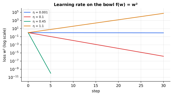
Reading it: each line is the loss (log scale) over 30 steps for one learning rate. The flat line near the top is 0.001: technically improving, practically stuck. 0.1 falls steadily. 0.45 falls fastest: its line ends at step 5, because one step later the loss is down to 10⁻¹², the floor of the chart. 1.1 climbs the whole way: every step makes things worse. On a real model you can't compute the perfect rate, so you look for the fastest one that doesn't blow up.
Level 3: the formula and its symbols
$$ w_{t+1} = w_t - \eta \cdot 2 w_t = (1 - 2\eta)\, w_t $$
Symbols
| Symbol | Meaning here | In the example |
|---|---|---|
| $2w_t$ | the slope of $w^2$ at $w_t$ | 2.0 at $w = 1$ |
| $1 - 2\eta$ | the factor each step multiplies $w$ by | −1.2 when $\eta = 1.1$ |
In words: "on this bowl, one step multiplies the weight by one minus twice the learning rate; if that factor's size is above 1, the weight grows instead of shrinking."
With the numbers: $\eta = 1.1$: $1 - 2.2 = -1.2$, so $1 \to -1.2 \to 1.44 \to -1.728$.
Level 3: in Python
In Python:
def three_steps(eta, w=1.0):
    out = []
    for t in range(3):
        # w - η·2w = (1 - 2η) w
        w = (1 - 2 * eta) * w
        out.append(round(w, 3))
    return out
three_steps(1.1)  # → [-1.2, 1.44, -1.728]
three_steps(0.1)  # → [0.8, 0.64, 0.512]
# η = 0.001 after 10 steps: barely moved
round(0.998 ** 10, 3)  # → 0.98
In code: descend_bowl is the same loop with the learning rate as an argument; call it with each rate in the table to reproduce every row.
Why it matters: the learning rate is the single most important hyperparameter. Too high and training diverges or bounces (loss spikes, NaNs); too low and it takes forever or settles somewhere poor. The steepest direction of the landscape sets the ceiling: on a bowl with slope 2w, any η above 1 diverges.
Momentum: a heavy ball instead of a cautious hiker
Now imagine a long, narrow valley: steep walls on both sides, a gentle slope along the floor. A cautious hiker who only reads the local slope zig-zags from wall to wall and barely moves along the floor. A heavy ball rolling down the same valley behaves differently: its sideways bouncing cancels out, while the gentle downhill pull along the floor keeps adding up, so it builds speed exactly where you want it. That accumulated speed is momentum.
Worked example on the bowl w², learning rate 0.1, momentum β = 0.9:
| step | slope g = 2w | velocity v = 0.9·v + g | new w = w − 0.1·v |
|---|---|---|---|
| 1 | 2.0 | 2.0 | 1.0 − 0.2 = 0.8 |
| 2 | 1.6 | 0.9 × 2.0 + 1.6 = 3.4 | 0.8 − 0.34 = 0.46 |
After two steps plain descent is at 0.64; momentum is already at 0.46.
flowchart LR
  G[Slope now g_t] --> V["Velocity v_t = β·v_(t−1) + g_t<br/>(remember 90% of the old speed)"]
  VO["Old velocity v_(t−1)"] --> V
  V --> S["Step: w − η·v_t"]
  S --> VO
Reading it: the velocity box mixes the new slope with 90% of the old velocity, and that velocity (not the raw slope) sets the step. Follow the loop back: next time, this velocity becomes the "old velocity". Slopes that keep pointing the same way pile up; slopes that flip sign every step (the walls) mostly cancel.
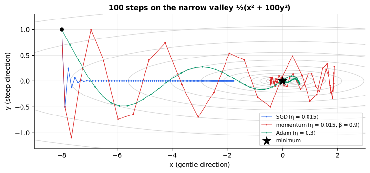
Reading it: the ellipses are contour lines of the valley ½(x² + 100y²), the start is at the left and the minimum is the star at the centre. Plain SGD (its learning rate capped by the steep walls) creeps along the floor and after 100 steps is still far from the star. Momentum swings hard: across the valley to y = −1.1 (further out than it started) and past the star to x ≈ 1.9, before the swings die down and it settles 0.003 from the minimum. Adam, which rescales each direction separately, takes a steadier line: it dips to y ≈ −0.5, overshoots to x ≈ 0.6, and ends 0.02 away. Both beat plain SGD by far; momentum's overshoot is the price of the speed it builds.
Level 3: the formula and its symbols
$$ v_t = \beta\, v_{t-1} + g_t, \qquad w_{t+1} = w_t - \eta\, v_t $$
Symbols
| Symbol | Meaning here | In the example |
|---|---|---|
| $g_t$ | the gradient (slope) at step $t$ | 2.0, then 1.6 |
| $v_t$ | the velocity: a running, fading sum of past gradients | 2.0, then 3.4 |
| $\beta$ | "beta", how much old velocity is kept each step (0 to 1) | 0.9 |
| $\eta$ | learning rate | 0.1 |
In words: "the velocity is 90% of the previous velocity plus the new slope, and the weights move by the learning rate times the velocity."
With the numbers: $v_2 = 0.9 \times 2.0 + 1.6 = 3.4$; $w_2 = 0.8 - 0.1 \times 3.4 = 0.46$.
Level 3: in Python
In Python:
w, v, beta, eta = 1.0, 0.0, 0.9, 0.1
for t in range(2):
    # the slope of w² here
    g = 2 * w
    # v_t = β v_(t-1) + g_t
    v = beta * v + g
    # w_(t+1) = w_t - η v_t
    w = w - eta * v
    print(round(v, 2), round(w, 2))  # → 2.0 0.8 3.4 0.46
In code: momentum_on_bowl runs the two-row table; SGD with a nonzero momentum keeps its velocity between calls to SGD.step. narrow_valley is the valley in the figure (rosenbrock is a harder, banana-shaped one), and run walks any optimizer across a landscape and records its path.
Why it matters: real loss surfaces are full of narrow valleys. On the valley above, 100 steps of momentum reach a loss over 10,000× lower than 100 steps of plain SGD at the same learning rate. Momentum is still the default for training CNNs.
Adam: a separate stride for every direction
Back in the narrow valley, what you'd really like is short steps across the steep walls and long strides along the gentle floor. Adam does exactly that: it keeps, for every single weight, a running average of the slope (the direction, like momentum) and a running average of the squared slope (how big that weight's slopes typically are), then divides the first by the square root of the second. Every weight ends up taking steps of roughly the same size, the learning rate, whatever the scale of its gradient.
Worked example: on its very first step, Adam moves a weight by exactly the learning rate (0.01 here), no matter whether that weight's gradient is 1000, 1 or 0.001. (With bias correction, m̂ = g and v̂ = g², so the step is 0.01 × g / |g| = 0.01.)
flowchart LR
  G[Gradient g] --> M["m: average of g<br/>(direction)"]
  G --> V["v: average of g²<br/>(typical size)"]
  M --> MC["m̂ = m / (1 − β1^t)"]
  V --> VC["v̂ = v / (1 − β2^t)"]
  MC --> D["step = η · m̂ / (√v̂ + ε)"]
  VC --> D
  D --> W[w − step]
Reading it: the gradient feeds two running averages. The top path remembers direction; the bottom path remembers magnitude. Both start at zero, so for the first few steps they're too small, and the "hat" boxes correct for that. The final box divides direction by typical size, which turns every weight's step into roughly η in the right direction.
Level 3: the formula and its symbols
$$ m_t = \beta_1 m_{t-1} + (1-\beta_1)\, g_t,\quad v_t = \beta_2 v_{t-1} + (1-\beta_2)\, g_t^2,\quad \hat{m}_t = \frac{m_t}{1-\beta_1^t},\quad \hat{v}_t = \frac{v_t}{1-\beta_2^t},\quad w_{t+1} = w_t - \eta\,\frac{\hat{m}_t}{\sqrt{\hat{v}_t} + \epsilon} $$
Symbols
| Symbol | Meaning here | In the example (first step, g = 1000) |
|---|---|---|
| $g_t$ | this weight's gradient at step $t$ | 1000 |
| $m_t$ | running average of the gradient ("first moment") | $0.1 \times 1000 = 100$ |
| $v_t$ | running average of the squared gradient ("second moment") | $0.001 \times 10^6 = 1000$ |
| $\beta_1, \beta_2$ | how much of the old averages to keep | 0.9, 0.999 |
| $\beta_1^t$ | $\beta_1$ raised to the step number | $0.9^1 = 0.9$ |
| $\hat{m}_t, \hat{v}_t$ | "m-hat, v-hat": the bias-corrected averages | 1000, $10^6$ |
| $\sqrt{\cdot}$ | square root | $\sqrt{10^6} = 1000$ |
| $\epsilon$ | "epsilon", a tiny number to avoid dividing by zero | $10^{-8}$ |
| $\eta$ | learning rate | 0.01 |
In words: "keep a running average of the gradient and of its square, correct both for starting at zero, then step by the learning rate times the average gradient divided by its typical size."
With the numbers: $\hat{m}_1 = 100 / 0.1 = 1000$, $\hat{v}_1 = 1000 / 0.001 = 10^6$, step $= 0.01 \times 1000 / (1000 + 10^{-8}) = 0.01$.
Level 3: in Python
In Python:
import math
beta_1, beta_2, eta, eps, t = 0.9, 0.999, 0.01, 1e-8, 1
def first_step(g):
    # m_1, starting from m_0 = 0
    m = beta_1 * 0 + (1 - beta_1) * g
    # v_1, starting from v_0 = 0
    v = beta_2 * 0 + (1 - beta_2) * g ** 2
    # undo the pull toward zero
    m_hat = m / (1 - beta_1 ** t)
    v_hat = v / (1 - beta_2 ** t)
    return eta * m_hat / (math.sqrt(v_hat) + eps)
# m_1, v_1
round((1 - beta_1) * 1000, 6), round((1 - beta_2) * 1000 ** 2, 6)  # → (100.0, 1000.0)
# the same step every time
[round(first_step(g), 6) for g in (1000, 1, 0.001)]  # → [0.01, 0.01, 0.01]
In code: Adam keeps the two running averages and the step count for every weight and applies the five formulas in Adam.step; adam_first_step shows the first step is always the learning rate.
Why it matters: Adam is forgiving: one learning rate works across weights whose gradients differ by orders of magnitude, which is the norm in transformers (embeddings, attention, layer norms all behave differently). On the valley above it reaches a loss below 10⁻¹⁰ in 300 steps while plain SGD is still around 10⁻³.
Weight decay, and why AdamW exists
Weight decay is a gentle leash that pulls every weight a little toward zero
each step, so the model prefers small, smooth weights over large, spiky ones
(a form of regularization; see primer.ml.regularization). The classic way
to add it was an L2 penalty: add λw to the gradient. With plain SGD that
is the same as shrinking the weight. With Adam it isn't, because Adam
divides the whole gradient, penalty included, by its typical size. The
leash's strength gets rescaled away.
Worked example: one step with zero loss-gradient, so only the decay acts. w = 1, learning rate 0.1.
| method | decay λ = 0.1 | decay λ = 0.001 |
|---|---|---|
| AdamW (decoupled) | 1 − 0.1 × 0.1 = 0.99 | 1 − 0.1 × 0.001 = 0.9999 |
| Adam with L2 in the gradient | 0.9 | 0.9 (the same!) |
With L2 inside Adam, a 100× weaker penalty shrinks the weight exactly as much: λ has stopped meaning what it says.
flowchart TB
  subgraph L2["Adam + L2 penalty"]
    g1[loss gradient] --> add["+ λ·w"] --> ad1[Adam rescaling<br/>÷ √v̂] --> s1[step]
  end
  subgraph AW["AdamW (decoupled)"]
    g2[loss gradient] --> ad2[Adam rescaling<br/>÷ √v̂] --> s2[step]
    w2[weights] --> dec["shrink: w − η·λ·w"] --> s2
  end
Reading it: on the left, the decay term joins the gradient before Adam's rescaling, so it gets divided by √v̂ like everything else and its strength is distorted. On the right (AdamW), the decay bypasses the rescaling and shrinks the weights directly, so λ means exactly "shrink by η·λ per step".
Level 3: the formula and its symbols
$$ \text{AdamW:}\quad w_{t+1} = w_t - \eta\,\frac{\hat{m}_t}{\sqrt{\hat{v}_t}+\epsilon} - \eta\,\lambda\, w_t $$
Symbols
| Symbol | Meaning here | In the example |
|---|---|---|
| $\lambda$ | "lambda", the weight-decay strength | 0.1 |
| $\eta\,\lambda\,w_t$ | how much the leash pulls this step | $0.1 \times 0.1 \times 1 = 0.01$ |
| $\hat{m}_t / (\sqrt{\hat{v}_t}+\epsilon)$ | Adam's usual step direction | 0 here (no loss gradient) |
In words: "take Adam's normal step, then separately shrink every weight by learning rate times decay times the weight."
With the numbers: $1 - 0 - 0.1 \times 0.1 \times 1 = 0.99$.
Level 3: in Python
In Python:
# no loss gradient: Adam's step is 0
w, eta, adam_step = 1.0, 0.1, 0.0
for lam in (0.1, 0.001):
    # AdamW: shrink by η λ w
    print(round(w - eta * adam_step - eta * lam * w, 4))  # → 0.99 0.9999
for lam in (0.1, 0.001):
    g = lam * w
    print(round(w - eta * g / abs(g), 4))  # → 0.9 0.9
In code: Adam implements both recipes: with decoupled decay it is AdamW, otherwise it adds the L2 penalty to the gradient. one_decay_step runs the table.
Why it matters: AdamW is the default optimizer for transformers. The fix was a one-line change that made weight decay behave predictably and improved generalization.
Warmup and cosine decay: easing on and off the gas
Think of driving an unfamiliar car. You ease onto the accelerator at first, because you don't yet know how it responds. You cruise at speed for most of the trip. Near the destination you slow gradually and glide into the parking spot. Transformers are trained the same way: the learning rate warms up linearly from 0 to its peak, then decays along a cosine curve toward a small floor.
Worked example with peak 0.001, 100 warmup steps, 1,000 steps total:
| step | phase | learning rate |
|---|---|---|
| 50 | halfway through warmup | 0.0005 |
| 100 | end of warmup | 0.001 (peak) |
| 550 | halfway through decay | 0.0005 |
| 1000 | end | the floor (e.g. 0.00001) |
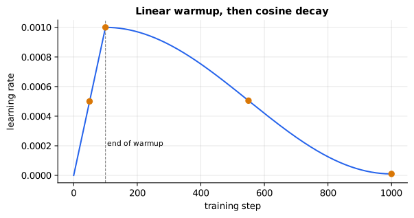
Reading it: the horizontal axis is the training step and the vertical axis the learning rate. The short straight ramp on the left is warmup. Then the curve rolls over the top, falls fastest in the middle and flattens as it approaches the floor, like half a cosine wave. The dots are the table above.
Level 3: the formula and its symbols
$$ \eta(t) = \begin{cases} \eta_{\max}\,\dfrac{t}{T_w} & t < T_w \[6pt] \eta_{\min} + (\eta_{\max}-\eta_{\min})\,\dfrac{1 + \cos!\left(\pi\,\dfrac{t - T_w}{T - T_w}\right)}{2} & t \ge T_w \end{cases} $$
Symbols
| Symbol | Meaning here | In the example |
|---|---|---|
| $\eta(t)$ | the learning rate at step $t$ | 0.0005 at $t = 550$ |
| $\eta_{\max}$ | the peak learning rate | 0.001 |
| $\eta_{\min}$ | the floor | 0 (or 0.00001) |
| $T_w$ | number of warmup steps | 100 |
| $T$ | total steps | 1000 |
| $\frac{t - T_w}{T - T_w}$ | progress through the decay, from 0 to 1 | $450/900 = 0.5$ |
| $\cos$ | cosine: 1 at 0, 0 at $\pi/2$, −1 at $\pi$ | $\cos(\pi/2) = 0$ |
| $\pi$ | pi, ≈ 3.1416 (half a turn, in radians) |
In words: "during warmup the rate climbs in a straight line to the peak; after that it follows half a cosine wave from the peak down to the floor."
With the numbers: step 550: progress 0.5, $\cos(0.5\pi) = 0$, so $0 + 0.001 \times (1 + 0)/2 = 0.0005$.
Level 3: in Python
In Python:
import math
eta_max, eta_min, T_w, T = 0.001, 0.0, 100, 1000
def eta(t):
    if t < T_w:
        # the straight ramp
        return eta_max * t / T_w
    # 0 to 1 through the decay
    progress = (t - T_w) / (T - T_w)
    return eta_min + (eta_max - eta_min) * (1 + math.cos(math.pi * progress)) / 2
[round(eta(t), 6) for t in (50, 100, 550, 1000)]  # → [0.0005, 0.001, 0.0005, 0.0]
In code: warmup_cosine returns the learning rate for any step: the straight ramp during warmup, then the half cosine down to the floor.
Why it matters: at the very start, Adam's averages are unreliable and the weights are random, so a full-size step can wreck them; warmup avoids early divergence. The slow finish lets the model settle into a good minimum instead of bouncing around it.
Gradient clipping: a speed limiter
Occasionally one bad batch produces an enormous gradient, a sudden cliff in the fog. Taking a full step along it could throw the weights far from anywhere useful. Clipping is a speed limiter: if the step would be longer than a set limit, shorten it to the limit, keeping its direction.
Worked example: the gradient (3, 4) has length √(3² + 4²) = 5. With a limit of 1, scale it by 1/5 to get (0.6, 0.8), length 1, same direction. A gradient of (0.3, 0.4) has length 0.5, under the limit, so it's left alone.
flowchart LR
  G[All gradients] --> N["Global length<br/>‖g‖ = √(sum of every squared entry)"]
  N --> C{"‖g‖ > limit?"}
  C -->|no| K[Use as is]
  C -->|yes| S["Multiply every gradient<br/>by limit / ‖g‖"]
  S --> K2[Same direction,<br/>length = limit]
Reading it: first measure the length of all the gradients together, as if they were one long list. If it's within the limit, nothing happens. If not, every gradient is multiplied by the same factor, which shortens the step without changing its direction.
Level 3: the formula and its symbols
$$ g \leftarrow g \cdot \min\left(1, \frac{c}{\lVert g \rVert}\right), \qquad \lVert g \rVert = \sqrt{\textstyle\sum_i g_i^2} $$
Symbols
| Symbol | Meaning here | In the example |
|---|---|---|
| $g$ | every gradient, treated as one long list | (3, 4) |
| $g_i$ | one entry of that list | 3, 4 |
| $\lVert g \rVert$ | the norm (length) of $g$: square every entry, add, take the square root | 5 |
| $c$ | the clipping limit | 1 |
| $\min(a, b)$ | the smaller of the two | $\min(1, 0.2) = 0.2$ |
In words: "if the gradient's length exceeds the limit, scale it down so its length equals the limit; otherwise leave it alone."
With the numbers: $(3, 4) \times \min(1, 1/5) = (0.6, 0.8)$.
Level 3: in Python
In Python:
import math
def clip(g, c):
    # ‖g‖ = √(Σ g_i²)
    norm = math.sqrt(sum(g_i ** 2 for g_i in g))
    # shrink only if too long
    scale = min(1, c / norm)
    return [round(g_i * scale, 2) for g_i in g]
clip([3, 4], c=1)  # → [0.6, 0.8]
# length 0.5: under the limit, left alone
clip([0.3, 0.4], c=1)  # → [0.3, 0.4]
In code: clip_by_global_norm measures the length of all gradients together and scales every one by the same factor when it exceeds the limit.
Why it matters: large-model training runs almost always clip (a limit of
1.0 is common). It turns rare loss spikes from run-ending disasters into
harmless blips. It's measured globally, across all layers together, so the
update's direction is preserved (see primer.ml.deep_nets for exploding
gradients).
In 20 seconds
- Gradient descent: step against the slope, scaled by the learning rate.
- The learning rate is the most important knob: too high diverges, too low stalls.
- Momentum accumulates a velocity so consistent directions speed up and zig-zags cancel.
- Adam gives every weight its own step size (average gradient ÷ its typical size); AdamW decouples weight decay from that rescaling and is the transformer default.
- Transformers use warmup then cosine decay, and clip gradients by global norm.
Self-test questions
What's the single most important hyperparameter, and what happens at each extreme? The learning rate. Too high: steps overshoot and training diverges or oscillates (loss spikes, NaNs). Too low: progress is so slow that training stalls or settles in a poor spot.
Why does momentum help in a narrow valley? Gradients across the valley flip sign every step and cancel in the velocity, while the small, consistent gradient along the valley accumulates, so the optimizer speeds up in the useful direction.
What does Adam's division by √v̂ achieve? It normalizes each weight's step by the typical size of its gradient, so every weight moves roughly η per step regardless of gradient scale. One learning rate then works for all parameters.
What's the difference between Adam with L2 and AdamW? With L2, the decay term is added to the gradient and then rescaled by Adam, so its effective strength varies per weight and λ loses its meaning. AdamW applies decay directly to the weights, outside the rescaling.
Why warm up the learning rate? At the start, weights are random and Adam's moment estimates are based on a handful of steps, so full-size updates can be wildly wrong and destabilize training. Ramping up gives the statistics time to settle.
What does gradient clipping protect against, and why clip the global norm? Rare huge gradients (exploding gradients, bad batches) that would throw the weights far off. Clipping the combined norm scales every tensor by the same factor, which preserves the update's direction.
The papers behind this lesson
- Kingma & Ba, Adam: A Method for Stochastic Optimization (2014): https://arxiv.org/abs/1412.6980 Combined momentum with per-weight step sizes and bias correction into the optimizer most networks are trained with. annotated companion
- Loshchilov & Hutter, Decoupled Weight Decay Regularization (AdamW, 2017): https://arxiv.org/abs/1711.05101 Showed that L2 regularization and weight decay differ under Adam, and fixed it by decoupling the decay.
- Sutskever, Martens, Dahl & Hinton, On the importance of initialization and momentum in deep learning (ICML 2013): https://proceedings.mlr.press/v28/sutskever13.html Demonstrated that well-tuned momentum makes plain SGD competitive on hard deep-network problems.
- Loshchilov & Hutter, SGDR: Stochastic Gradient Descent with Warm Restarts (2016): https://arxiv.org/abs/1608.03983 Introduced cosine learning-rate annealing, now the standard decay shape.
- Pascanu, Mikolov & Bengio, On the difficulty of training recurrent neural networks (2012): https://arxiv.org/abs/1211.5063 Analysed exploding gradients and proposed clipping the gradient norm.
Further reading
- Sebastian Ruder, An overview of gradient descent optimization algorithms: https://arxiv.org/abs/1609.04747
- Gabriel Goh, Why Momentum Really Works (Distill): https://distill.pub/2017/momentum/
- Kingma & Ba, Adam: A Method for Stochastic Optimization (2014): https://arxiv.org/abs/1412.6980
- Loshchilov & Hutter, Decoupled Weight Decay Regularization (AdamW, 2017): https://arxiv.org/abs/1711.05101
- Loshchilov & Hutter, SGDR: Stochastic Gradient Descent with Warm Restarts (cosine schedules, 2016): https://arxiv.org/abs/1608.03983
- Pascanu, Mikolov & Bengio, On the difficulty of training recurrent neural networks (gradient clipping, 2012): https://arxiv.org/abs/1211.5063
- CS231n notes, Neural Networks Part 3 (parameter updates): https://cs231n.github.io/neural-networks-3/
- PyTorch
torch.optimdocs: https://pytorch.org/docs/stable/optim.html
1r""" 2# Optimizers: how weights take their steps downhill 3 4Run: `python -m primer.ml.optimizers` 5 6New to the notation (∇, η, β)? `primer.notation` builds every symbol used 7here from zero. This lesson builds on the training loop and the gradient 8from `primer.ml.neural_net`. 9 10## Level 1: The practitioner's guide 11 12**In one sentence.** An optimizer is the rule that turns "the slope of the 13loss here" into "the step every weight takes", and the handful of settings 14that come with it (learning rate, momentum, the two Adam betas, weight 15decay, warmup, clipping) are most of what a training recipe consists of. 16 17**When you need it.** You need this the moment a training or fine-tuning 18job asks you for a learning rate, and again the first time a loss curve 19spikes, turns NaN, or flattens long before the model is any good. The tell: 20a config with `lr`, `betas`, `weight_decay`, `warmup_steps` and 21`max_grad_norm` copied from someone else's run, and a paper's training 22section that reads as Greek (β₁ = 0.9, β₂ = 0.95, ε = 10⁻⁵) rather than as 23choices. You don't need it to call a trained model, and a hosted 24fine-tuning API chooses the optimizer for you; what you set there is the 25learning rate and how long to train, which is still the most important 26choice on this page. One number from this lesson shows how much the rule 27matters: in a narrow valley, 100 steps of momentum reach a loss more than 2810,000 times lower than 100 steps of plain gradient descent at the same 29learning rate. 30 31**Your options.** The rules, plus two add-ons that ride on any of them, 32from the simplest to the one transformers use: 33 34| Option | What it does | What it guarantees | What it costs | Where it lives | 35|---|---|---|---|---| 36| Plain SGD | Steps against the current batch's slope, scaled by the learning rate | The simplest rule, nothing to tune but η | The steepest direction caps η, so it creeps along gentle valley floors: loss 1.56 after 100 steps here | Your training script, no extra memory | 37| SGD with momentum | Keeps a velocity: 90% of the last one plus the new slope | Consistent directions speed up and zig-zags cancel: loss 6.5 × 10⁻⁵ after the same 100 steps | One extra number per weight, and overshoot past the minimum before it settles | The default for CNNs | 38| Adam | Gives every weight its own step: its average gradient divided by its typical gradient size; the first step is exactly η whatever the gradient | One learning rate works across weights whose gradients differ by orders of magnitude | Two extra numbers per weight; unreliable averages in the first steps; an L2 penalty added to its gradient loses its meaning | Most training scripts | 39| AdamW | Adam, with weight decay applied straight to the weights instead of through the gradient | λ means what it says: shrink by η × λ per step | The same memory as Adam | The transformer default; PyTorch's `AdamW` ships with lr 0.001, betas (0.9, 0.999), eps 10⁻⁸, weight_decay 0.01 | 40| Warmup then decay (a schedule on top) | Ramps η from 0 to its peak, then lowers it along a cosine or a straight line to a floor | No full-size steps while the weights are random and Adam's averages unsettled; a gentle finish into a good minimum | Two more settings, warmup steps and total steps, so the run's length must be known up front | The scheduler | 41| Gradient clipping (on top) | Rescales the whole gradient when its combined length exceeds a limit, direction unchanged | A rare spike becomes a blip instead of a wrecked run | One norm per step; it can hide a network that explodes every step | One line before the optimizer step | 42 43**How to choose.** Start from the architecture, then from the size. 44 45- A transformer, pretraining or fine-tuning: AdamW, warmup, a cosine or 46 linear decay, clipping at 1.0. That is the Llama 2 recipe (AdamW with 47 β₁ = 0.9, β₂ = 0.95, ε = 10⁻⁵, 2000 warmup steps, cosine decay to 10% of 48 the peak, weight decay 0.1, clipping 1.0) and the shape of Hugging Face's 49 `TrainingArguments` defaults (AdamW, a linear schedule, max_grad_norm 50 1.0). 51- A convolutional network: SGD with momentum 0.9, still the default there. 52- The learning rate itself: the fastest one that doesn't blow up, found by 53 trying a few. Bigger models take smaller rates (Llama 2 uses 3 × 10⁻⁴ for 54 its 7B and 13B models and 1.5 × 10⁻⁴ for 34B and 70B), and fine-tuning 55 takes smaller rates than pretraining (Hugging Face defaults to 5 × 10⁻⁵). 56- A published recipe you are reproducing: copy every setting, betas 57 included. The transformer paper's β₂ = 0.98 and Llama 2's 0.95 are both 58 deliberate departures from Adam's 0.999. 59- Whatever you pick, the learning rate is the single most important 60 hyperparameter, and a schedule is part of it: the peak, the warmup and 61 the total steps are one decision. 62 63**What it costs.** Memory: momentum keeps one extra number per weight and 64Adam or AdamW keep two, so the optimizer state of a large model is twice 65the size of the weights it trains, which is a large part of why training 66needs more memory than serving. Compute: a few operations per weight per 67step, small beside the forward and backward passes. Time: warmup and decay 68need the total step count, so the budget is fixed before the run starts, 69and a run stopped halfway never reached its low learning rate. Quality: 70on this lesson's narrow valley, after 300 steps plain SGD sits at a loss 71of 3.7 × 10⁻³, Adam at 1.1 × 10⁻¹¹ and momentum at 1.8 × 10⁻¹²; the rule 72decides whether a fixed budget of steps gets there at all. 73 74**What breaks.** 75 76- **Loss spikes, then NaN.** The learning rate is too high: on a bowl with 77 slope 2w, any η above 1 makes every step overshoot further than the last. 78 Lower it, add warmup, clip. 79- **Loss barely moves.** Too low: at η = 0.001 the bowl's weight is still at 80 0.98 after ten steps. Raise it until training becomes unstable, then 81 back off. 82- **Weight decay that does nothing, or too much.** An L2 penalty inside 83 Adam gets divided by the typical gradient size, so λ = 0.1 and λ = 0.001 84 shrink a weight by the same amount. Use AdamW, where λ = 0.1 means 0.99 85 per step and 0.001 means 0.9999. 86- **Divergence in the first hundred steps with Adam.** No warmup: its 87 averages are built from a handful of steps and the weights are random. 88- **Overshoot.** Momentum swings hard, across the valley and past the 89 minimum, before it settles; the trajectory figure in Level 2 shows it. A 90 smaller β or a smaller η calms it. 91- **Clipping on every step.** The gradient is exploding, not spiking; the 92 fix is initialization or normalization (`primer.ml.deep_nets`), and 93 clipping is hiding it. 94- **A schedule cut short.** Cosine decay reaches its floor only at the 95 planned last step; stop early and the model never settled. 96 97**In the wild.** *Attention Is All You Need* trained with Adam at β₁ = 0.9, 98β₂ = 0.98, ε = 10⁻⁹, a learning rate that rises linearly for 4000 warmup 99steps and then falls with the inverse square root of the step. Llama 2 100used AdamW with the recipe above. PyTorch ships `torch.optim.SGD` 101(momentum as an argument), `Adam` and `AdamW`, and clips with 102`torch.nn.utils.clip_grad_norm_`, which measures the norm over all 103parameters "as if the norms of the individual gradients were concatenated 104into a single vector". Hugging Face's `TrainingArguments` defaults to 105AdamW (`adamw_torch_fused` on recent PyTorch), learning_rate 5e-5, 106weight_decay 0.0, betas 0.9 and 0.999, epsilon 1e-8, a linear schedule 107with no warmup and max_grad_norm 1.0. The rules come from Kingma and Ba 108(Adam, 2014), Loshchilov and Hutter (AdamW, 2017, and cosine annealing, 1092016), Sutskever et al. (momentum, 2013) and Pascanu et al. (clipping, 1102012), all linked at the end of the lesson. 111 112**Go deeper.** Level 2 walks each rule down the same bowl with two-row 113tables you can check by hand, races SGD, momentum and Adam across a narrow 114valley, shows why an L2 penalty inside Adam stops meaning anything, draws 115the warmup-and-cosine curve, and clips (3, 4) down to (0.6, 0.8). If you 116only needed to fill in a config, you are done. 117 118## Level 2: How it works, from scratch 119 120Every optimizer runs the same loop: feel the slope, turn it into a step, 121take it, repeat. This level builds each rule on a one-number valley you 122can check by hand, then lets them race across a valley that is not round. 123 124## The idea: walking downhill in fog 125 126You're on a hillside in thick fog and want to reach the lowest point in the 127valley. You can't see the valley; you can only feel the slope under your 128feet. So you feel which way is downhill, take a step that way, and repeat. 129That is **gradient descent**. The hillside is the loss (how wrong the model 130is, for every possible setting of its weights), your position is the 131current weights, and the slope under your feet is the **gradient**: the list 132of slopes of the loss, one per weight. (See `primer.ml.neural_net` for how 133backprop measures it, and `primer.notation` for the symbols.) An 134**optimizer** is your rule for turning "the slope here" into "the step I 135take". 136 137Worked example on the simplest possible valley, the bowl f(w) = w², whose 138slope at w is 2w. Start at w = 1 with step size 0.1: 139 140| step | w | slope 2w | step taken 0.1 × slope | new w | 141|---|---|---|---|---| 142| 0 | 1.0 | 2.0 | 0.2 | 0.8 | 143| 1 | 0.8 | 1.6 | 0.16 | 0.64 | 144 145Each step keeps 80% of w, sliding smoothly toward the bottom at 0. 146 147```mermaid 148flowchart LR 149 W[Current weights] --> G[Feel the slope<br/>compute gradient] 150 G --> R{Optimizer rule} 151 R --> S[Step] 152 S --> W2[New weights] 153 W2 -->|repeat| G 154 R -.uses.-> H[Its own memory:<br/>velocity, averages] 155``` 156 157**Reading it:** every optimizer runs this loop; they differ only in the 158diamond. Plain gradient descent's rule looks only at the current slope. 159Momentum and Adam also keep a small memory of past slopes (the dotted box) 160and use it to choose a better step. 161 162$$ 163w_{t+1} = w_t - \eta \, \nabla \mathcal{L}(w_t) 164$$ 165 166**Symbols** 167 168| Symbol | Meaning here | In the example | 169|---|---|---| 170| $w_t$ | the weights at step $t$ | $w_0 = 1.0$ | 171| $t$ | the step counter | 0, 1, 2, … | 172| $\eta$ | "eta", the learning rate (step size) | 0.1 | 173| $\mathcal{L}$ | the loss | $w^2$ | 174| $\nabla \mathcal{L}(w_t)$ | "nabla L", the gradient: the slope of the loss at the current weights, one number per weight | $2 \times 1.0 = 2.0$ | 175 176**In words:** "the next weights are the current weights minus the learning 177rate times the slope of the loss where we stand." 178 179**With the numbers:** $w_1 = 1.0 - 0.1 \times 2.0 = 0.8$; 180$w_2 = 0.8 - 0.1 \times 1.6 = 0.64$. 181 182**In Python:** 183 184```python 185w, eta = 1.0, 0.1 186# ∇L for the bowl L = w² 187def grad_L(w): return 2 * w 188for t in range(2): 189 # w_(t+1) = w_t - η ∇L(w_t) 190 w = w - eta * grad_L(w) 191 print(round(w, 2)) # → 0.8 0.64 192``` 193 194"Stochastic" gradient descent (SGD) means the slope is estimated from a 195small random batch of examples instead of the whole dataset: noisier, but 196thousands of times cheaper per step. `descend_bowl` runs the table above; 197`SGD` is the general version. 198 199**Why it matters:** every model you've heard of was trained by a descendant 200of this one line. The variants below exist because real loss landscapes are 201not round bowls. 202 203## The learning rate: how long a stride? 204 205In the fog, stride length is everything. Tiny shuffling steps are safe but 206you'll be walking all night. Giant leaps overshoot the valley floor and land 207you higher up the opposite slope; keep leaping and you climb out of the 208valley altogether. 209 210Worked example on the bowl w², where each step multiplies w by (1 − 2η): 211 212| learning rate η | multiplier 1 − 2η | w after 1, 2, 3 steps | what happens | 213|---|---|---|---| 214| 0.001 | 0.998 | 0.998, 0.996, 0.994 | stalls: 10 steps only reach 0.980 | 215| 0.1 | 0.8 | 0.8, 0.64, 0.512 | smooth progress | 216| 0.5 | 0 | 0, 0, 0 | lands on the bottom in one step | 217| 1.1 | −1.2 | −1.2, 1.44, −1.728 | overshoots further each time: diverges | 218 219 220 221**Reading it:** each line is the loss (log scale) over 30 steps for one 222learning rate. The flat line near the top is 0.001: technically improving, 223practically stuck. 0.1 falls steadily. 0.45 falls fastest: its line ends at 224step 5, because one step later the loss is down to 10⁻¹², the floor of the chart. 2251.1 climbs the whole way: every step makes things worse. On a real model you 226can't compute the perfect rate, so you look for the fastest one that doesn't 227blow up. 228 229$$ 230w_{t+1} = w_t - \eta \cdot 2 w_t = (1 - 2\eta)\, w_t 231$$ 232 233**Symbols** 234 235| Symbol | Meaning here | In the example | 236|---|---|---| 237| $2w_t$ | the slope of $w^2$ at $w_t$ | 2.0 at $w = 1$ | 238| $1 - 2\eta$ | the factor each step multiplies $w$ by | −1.2 when $\eta = 1.1$ | 239 240**In words:** "on this bowl, one step multiplies the weight by one minus 241twice the learning rate; if that factor's size is above 1, the weight grows 242instead of shrinking." 243 244**With the numbers:** $\eta = 1.1$: $1 - 2.2 = -1.2$, so 245$1 \to -1.2 \to 1.44 \to -1.728$. 246 247**In Python:** 248 249```python 250def three_steps(eta, w=1.0): 251 out = [] 252 for t in range(3): 253 # w - η·2w = (1 - 2η) w 254 w = (1 - 2 * eta) * w 255 out.append(round(w, 3)) 256 return out 257three_steps(1.1) # → [-1.2, 1.44, -1.728] 258three_steps(0.1) # → [0.8, 0.64, 0.512] 259# η = 0.001 after 10 steps: barely moved 260round(0.998 ** 10, 3) # → 0.98 261``` 262 263**In code:** `descend_bowl` is the same loop with the learning rate as an argument; call it with each rate in the table to reproduce every row. 264 265**Why it matters:** the learning rate is the single most important 266hyperparameter. Too high and training diverges or bounces (loss spikes, 267NaNs); too low and it takes forever or settles somewhere poor. The steepest 268direction of the landscape sets the ceiling: on a bowl with slope 2w, any η 269above 1 diverges. 270 271## Momentum: a heavy ball instead of a cautious hiker 272 273Now imagine a long, narrow valley: steep walls on both sides, a gentle slope 274along the floor. A cautious hiker who only reads the local slope zig-zags 275from wall to wall and barely moves along the floor. A heavy ball rolling 276down the same valley behaves differently: its sideways bouncing cancels out, 277while the gentle downhill pull along the floor keeps adding up, so it builds 278speed exactly where you want it. That accumulated speed is **momentum**. 279 280Worked example on the bowl w², learning rate 0.1, momentum β = 0.9: 281 282| step | slope g = 2w | velocity v = 0.9·v + g | new w = w − 0.1·v | 283|---|---|---|---| 284| 1 | 2.0 | 2.0 | 1.0 − 0.2 = 0.8 | 285| 2 | 1.6 | 0.9 × 2.0 + 1.6 = 3.4 | 0.8 − 0.34 = 0.46 | 286 287After two steps plain descent is at 0.64; momentum is already at 0.46. 288 289```mermaid 290flowchart LR 291 G[Slope now g_t] --> V["Velocity v_t = β·v_(t−1) + g_t<br/>(remember 90% of the old speed)"] 292 VO["Old velocity v_(t−1)"] --> V 293 V --> S["Step: w − η·v_t"] 294 S --> VO 295``` 296 297**Reading it:** the velocity box mixes the new slope with 90% of the old 298velocity, and that velocity (not the raw slope) sets the step. Follow the 299loop back: next time, this velocity becomes the "old velocity". Slopes that 300keep pointing the same way pile up; slopes that flip sign every step (the 301walls) mostly cancel. 302 303 304 305**Reading it:** the ellipses are contour lines of the valley ½(x² + 100y²), 306the start is at the left and the minimum is the star at the centre. Plain 307SGD (its learning rate capped by the steep walls) creeps along the floor and 308after 100 steps is still far from the star. Momentum swings hard: across 309the valley to y = −1.1 (further out than it started) and past the star to 310x ≈ 1.9, before the swings die down and it settles 0.003 from the minimum. 311Adam, which rescales each direction separately, takes a steadier line: it 312dips to y ≈ −0.5, overshoots to x ≈ 0.6, and ends 0.02 away. Both beat 313plain SGD by far; momentum's overshoot is the price of the speed it builds. 314 315$$ 316v_t = \beta\, v_{t-1} + g_t, \qquad w_{t+1} = w_t - \eta\, v_t 317$$ 318 319**Symbols** 320 321| Symbol | Meaning here | In the example | 322|---|---|---| 323| $g_t$ | the gradient (slope) at step $t$ | 2.0, then 1.6 | 324| $v_t$ | the velocity: a running, fading sum of past gradients | 2.0, then 3.4 | 325| $\beta$ | "beta", how much old velocity is kept each step (0 to 1) | 0.9 | 326| $\eta$ | learning rate | 0.1 | 327 328**In words:** "the velocity is 90% of the previous velocity plus the new 329slope, and the weights move by the learning rate times the velocity." 330 331**With the numbers:** $v_2 = 0.9 \times 2.0 + 1.6 = 3.4$; 332$w_2 = 0.8 - 0.1 \times 3.4 = 0.46$. 333 334**In Python:** 335 336```python 337w, v, beta, eta = 1.0, 0.0, 0.9, 0.1 338for t in range(2): 339 # the slope of w² here 340 g = 2 * w 341 # v_t = β v_(t-1) + g_t 342 v = beta * v + g 343 # w_(t+1) = w_t - η v_t 344 w = w - eta * v 345 print(round(v, 2), round(w, 2)) # → 2.0 0.8 3.4 0.46 346``` 347 348**In code:** `momentum_on_bowl` runs the two-row table; `SGD` with a nonzero momentum keeps its velocity between calls to `SGD.step`. `narrow_valley` is the valley in the figure (`rosenbrock` is a harder, banana-shaped one), and `run` walks any optimizer across a landscape and records its path. 349 350**Why it matters:** real loss surfaces are full of narrow valleys. On the 351valley above, 100 steps of momentum reach a loss over 10,000× lower than 100 352steps of plain SGD at the same learning rate. Momentum is still the default 353for training CNNs. 354 355## Adam: a separate stride for every direction 356 357Back in the narrow valley, what you'd really like is short steps across the 358steep walls and long strides along the gentle floor. Adam does exactly that: 359it keeps, for every single weight, a running average of the slope (the 360direction, like momentum) and a running average of the *squared* slope (how 361big that weight's slopes typically are), then divides the first by the 362square root of the second. Every weight ends up taking steps of roughly the 363same size, the learning rate, whatever the scale of its gradient. 364 365Worked example: on its very first step, Adam moves a weight by exactly the 366learning rate (0.01 here), no matter whether that weight's gradient is 1000, 3671 or 0.001. (With bias correction, m̂ = g and v̂ = g², so the step is 3680.01 × g / |g| = 0.01.) 369 370```mermaid 371flowchart LR 372 G[Gradient g] --> M["m: average of g<br/>(direction)"] 373 G --> V["v: average of g²<br/>(typical size)"] 374 M --> MC["m̂ = m / (1 − β1^t)"] 375 V --> VC["v̂ = v / (1 − β2^t)"] 376 MC --> D["step = η · m̂ / (√v̂ + ε)"] 377 VC --> D 378 D --> W[w − step] 379``` 380 381**Reading it:** the gradient feeds two running averages. The top path 382remembers direction; the bottom path remembers magnitude. Both start at 383zero, so for the first few steps they're too small, and the "hat" boxes 384correct for that. The final box divides direction by typical size, which 385turns every weight's step into roughly η in the right direction. 386 387$$ 388m_t = \beta_1 m_{t-1} + (1-\beta_1)\, g_t,\quad 389v_t = \beta_2 v_{t-1} + (1-\beta_2)\, g_t^2,\quad 390\hat{m}_t = \frac{m_t}{1-\beta_1^t},\quad 391\hat{v}_t = \frac{v_t}{1-\beta_2^t},\quad 392w_{t+1} = w_t - \eta\,\frac{\hat{m}_t}{\sqrt{\hat{v}_t} + \epsilon} 393$$ 394 395**Symbols** 396 397| Symbol | Meaning here | In the example (first step, g = 1000) | 398|---|---|---| 399| $g_t$ | this weight's gradient at step $t$ | 1000 | 400| $m_t$ | running average of the gradient ("first moment") | $0.1 \times 1000 = 100$ | 401| $v_t$ | running average of the squared gradient ("second moment") | $0.001 \times 10^6 = 1000$ | 402| $\beta_1, \beta_2$ | how much of the old averages to keep | 0.9, 0.999 | 403| $\beta_1^t$ | $\beta_1$ raised to the step number | $0.9^1 = 0.9$ | 404| $\hat{m}_t, \hat{v}_t$ | "m-hat, v-hat": the bias-corrected averages | 1000, $10^6$ | 405| $\sqrt{\cdot}$ | square root | $\sqrt{10^6} = 1000$ | 406| $\epsilon$ | "epsilon", a tiny number to avoid dividing by zero | $10^{-8}$ | 407| $\eta$ | learning rate | 0.01 | 408 409**In words:** "keep a running average of the gradient and of its square, 410correct both for starting at zero, then step by the learning rate times the 411average gradient divided by its typical size." 412 413**With the numbers:** $\hat{m}_1 = 100 / 0.1 = 1000$, $\hat{v}_1 = 1000 / 0.001 = 10^6$, 414step $= 0.01 \times 1000 / (1000 + 10^{-8}) = 0.01$. 415 416**In Python:** 417 418```python 419import math 420beta_1, beta_2, eta, eps, t = 0.9, 0.999, 0.01, 1e-8, 1 421def first_step(g): 422 # m_1, starting from m_0 = 0 423 m = beta_1 * 0 + (1 - beta_1) * g 424 # v_1, starting from v_0 = 0 425 v = beta_2 * 0 + (1 - beta_2) * g ** 2 426 # undo the pull toward zero 427 m_hat = m / (1 - beta_1 ** t) 428 v_hat = v / (1 - beta_2 ** t) 429 return eta * m_hat / (math.sqrt(v_hat) + eps) 430# m_1, v_1 431round((1 - beta_1) * 1000, 6), round((1 - beta_2) * 1000 ** 2, 6) # → (100.0, 1000.0) 432# the same step every time 433[round(first_step(g), 6) for g in (1000, 1, 0.001)] # → [0.01, 0.01, 0.01] 434``` 435 436**In code:** `Adam` keeps the two running averages and the step count for every weight and applies the five formulas in `Adam.step`; `adam_first_step` shows the first step is always the learning rate. 437 438**Why it matters:** Adam is forgiving: one learning rate works across 439weights whose gradients differ by orders of magnitude, which is the norm in 440transformers (embeddings, attention, layer norms all behave differently). 441On the valley above it reaches a loss below 10⁻¹⁰ in 300 steps while plain 442SGD is still around 10⁻³. 443 444## Weight decay, and why AdamW exists 445 446Weight decay is a gentle leash that pulls every weight a little toward zero 447each step, so the model prefers small, smooth weights over large, spiky ones 448(a form of regularization; see `primer.ml.regularization`). The classic way 449to add it was an **L2 penalty**: add λw to the gradient. With plain SGD that 450is the same as shrinking the weight. With Adam it isn't, because Adam 451divides the whole gradient, penalty included, by its typical size. The 452leash's strength gets rescaled away. 453 454Worked example: one step with zero loss-gradient, so only the decay acts. 455w = 1, learning rate 0.1. 456 457| method | decay λ = 0.1 | decay λ = 0.001 | 458|---|---|---| 459| AdamW (decoupled) | 1 − 0.1 × 0.1 = **0.99** | 1 − 0.1 × 0.001 = **0.9999** | 460| Adam with L2 in the gradient | **0.9** | **0.9** (the same!) | 461 462With L2 inside Adam, a 100× weaker penalty shrinks the weight exactly as 463much: λ has stopped meaning what it says. 464 465```mermaid 466flowchart TB 467 subgraph L2["Adam + L2 penalty"] 468 g1[loss gradient] --> add["+ λ·w"] --> ad1[Adam rescaling<br/>÷ √v̂] --> s1[step] 469 end 470 subgraph AW["AdamW (decoupled)"] 471 g2[loss gradient] --> ad2[Adam rescaling<br/>÷ √v̂] --> s2[step] 472 w2[weights] --> dec["shrink: w − η·λ·w"] --> s2 473 end 474``` 475 476**Reading it:** on the left, the decay term joins the gradient *before* 477Adam's rescaling, so it gets divided by √v̂ like everything else and its 478strength is distorted. On the right (AdamW), the decay bypasses the 479rescaling and shrinks the weights directly, so λ means exactly "shrink by 480η·λ per step". 481 482$$ 483\text{AdamW:}\quad w_{t+1} = w_t - \eta\,\frac{\hat{m}_t}{\sqrt{\hat{v}_t}+\epsilon} - \eta\,\lambda\, w_t 484$$ 485 486**Symbols** 487 488| Symbol | Meaning here | In the example | 489|---|---|---| 490| $\lambda$ | "lambda", the weight-decay strength | 0.1 | 491| $\eta\,\lambda\,w_t$ | how much the leash pulls this step | $0.1 \times 0.1 \times 1 = 0.01$ | 492| $\hat{m}_t / (\sqrt{\hat{v}_t}+\epsilon)$ | Adam's usual step direction | 0 here (no loss gradient) | 493 494**In words:** "take Adam's normal step, then separately shrink every 495weight by learning rate times decay times the weight." 496 497**With the numbers:** $1 - 0 - 0.1 \times 0.1 \times 1 = 0.99$. 498 499**In Python:** 500 501```python 502# no loss gradient: Adam's step is 0 503w, eta, adam_step = 1.0, 0.1, 0.0 504for lam in (0.1, 0.001): 505 # AdamW: shrink by η λ w 506 print(round(w - eta * adam_step - eta * lam * w, 4)) # → 0.99 0.9999 507for lam in (0.1, 0.001): 508 g = lam * w 509 print(round(w - eta * g / abs(g), 4)) # → 0.9 0.9 510``` 511 512**In code:** `Adam` implements both recipes: with decoupled decay it is AdamW, otherwise it adds the L2 penalty to the gradient. `one_decay_step` runs the table. 513 514**Why it matters:** AdamW is the default optimizer for transformers. The 515fix was a one-line change that made weight decay behave predictably and 516improved generalization. 517 518## Warmup and cosine decay: easing on and off the gas 519 520Think of driving an unfamiliar car. You ease onto the accelerator at first, 521because you don't yet know how it responds. You cruise at speed for most of 522the trip. Near the destination you slow gradually and glide into the 523parking spot. Transformers are trained the same way: the learning rate 524**warms up** linearly from 0 to its peak, then **decays** along a cosine 525curve toward a small floor. 526 527Worked example with peak 0.001, 100 warmup steps, 1,000 steps total: 528 529| step | phase | learning rate | 530|---|---|---| 531| 50 | halfway through warmup | 0.0005 | 532| 100 | end of warmup | 0.001 (peak) | 533| 550 | halfway through decay | 0.0005 | 534| 1000 | end | the floor (e.g. 0.00001) | 535 536 537 538**Reading it:** the horizontal axis is the training step and the vertical 539axis the learning rate. The short straight ramp on the left is warmup. Then 540the curve rolls over the top, falls fastest in the middle and flattens as it 541approaches the floor, like half a cosine wave. The dots are the table above. 542 543$$ 544\eta(t) = 545\begin{cases} 546\eta_{\max}\,\dfrac{t}{T_w} & t < T_w \\[6pt] 547\eta_{\min} + (\eta_{\max}-\eta_{\min})\,\dfrac{1 + \cos\!\left(\pi\,\dfrac{t - T_w}{T - T_w}\right)}{2} & t \ge T_w 548\end{cases} 549$$ 550 551**Symbols** 552 553| Symbol | Meaning here | In the example | 554|---|---|---| 555| $\eta(t)$ | the learning rate at step $t$ | 0.0005 at $t = 550$ | 556| $\eta_{\max}$ | the peak learning rate | 0.001 | 557| $\eta_{\min}$ | the floor | 0 (or 0.00001) | 558| $T_w$ | number of warmup steps | 100 | 559| $T$ | total steps | 1000 | 560| $\frac{t - T_w}{T - T_w}$ | progress through the decay, from 0 to 1 | $450/900 = 0.5$ | 561| $\cos$ | cosine: 1 at 0, 0 at $\pi/2$, −1 at $\pi$ | $\cos(\pi/2) = 0$ | 562| $\pi$ | pi, ≈ 3.1416 (half a turn, in radians) | | 563 564**In words:** "during warmup the rate climbs in a straight line to the peak; 565after that it follows half a cosine wave from the peak down to the floor." 566 567**With the numbers:** step 550: progress 0.5, $\cos(0.5\pi) = 0$, so 568$0 + 0.001 \times (1 + 0)/2 = 0.0005$. 569 570**In Python:** 571 572```python 573import math 574eta_max, eta_min, T_w, T = 0.001, 0.0, 100, 1000 575def eta(t): 576 if t < T_w: 577 # the straight ramp 578 return eta_max * t / T_w 579 # 0 to 1 through the decay 580 progress = (t - T_w) / (T - T_w) 581 return eta_min + (eta_max - eta_min) * (1 + math.cos(math.pi * progress)) / 2 582[round(eta(t), 6) for t in (50, 100, 550, 1000)] # → [0.0005, 0.001, 0.0005, 0.0] 583``` 584 585**In code:** `warmup_cosine` returns the learning rate for any step: the straight ramp during warmup, then the half cosine down to the floor. 586 587**Why it matters:** at the very start, Adam's averages are unreliable and 588the weights are random, so a full-size step can wreck them; warmup avoids 589early divergence. The slow finish lets the model settle into a good minimum 590instead of bouncing around it. 591 592## Gradient clipping: a speed limiter 593 594Occasionally one bad batch produces an enormous gradient, a sudden cliff in 595the fog. Taking a full step along it could throw the weights far from 596anywhere useful. Clipping is a speed limiter: if the step would be longer 597than a set limit, shorten it to the limit, keeping its direction. 598 599Worked example: the gradient (3, 4) has length √(3² + 4²) = 5. With a limit 600of 1, scale it by 1/5 to get (0.6, 0.8), length 1, same direction. A gradient 601of (0.3, 0.4) has length 0.5, under the limit, so it's left alone. 602 603```mermaid 604flowchart LR 605 G[All gradients] --> N["Global length<br/>‖g‖ = √(sum of every squared entry)"] 606 N --> C{"‖g‖ > limit?"} 607 C -->|no| K[Use as is] 608 C -->|yes| S["Multiply every gradient<br/>by limit / ‖g‖"] 609 S --> K2[Same direction,<br/>length = limit] 610``` 611 612**Reading it:** first measure the length of *all* the gradients together, 613as if they were one long list. If it's within the limit, nothing happens. 614If not, every gradient is multiplied by the same factor, which shortens the 615step without changing its direction. 616 617$$ 618g \leftarrow g \cdot \min\left(1, \frac{c}{\lVert g \rVert}\right), \qquad 619\lVert g \rVert = \sqrt{\textstyle\sum_i g_i^2} 620$$ 621 622**Symbols** 623 624| Symbol | Meaning here | In the example | 625|---|---|---| 626| $g$ | every gradient, treated as one long list | (3, 4) | 627| $g_i$ | one entry of that list | 3, 4 | 628| $\lVert g \rVert$ | the **norm** (length) of $g$: square every entry, add, take the square root | 5 | 629| $c$ | the clipping limit | 1 | 630| $\min(a, b)$ | the smaller of the two | $\min(1, 0.2) = 0.2$ | 631 632**In words:** "if the gradient's length exceeds the limit, scale it down so 633its length equals the limit; otherwise leave it alone." 634 635**With the numbers:** $(3, 4) \times \min(1, 1/5) = (0.6, 0.8)$. 636 637**In Python:** 638 639```python 640import math 641def clip(g, c): 642 # ‖g‖ = √(Σ g_i²) 643 norm = math.sqrt(sum(g_i ** 2 for g_i in g)) 644 # shrink only if too long 645 scale = min(1, c / norm) 646 return [round(g_i * scale, 2) for g_i in g] 647clip([3, 4], c=1) # → [0.6, 0.8] 648# length 0.5: under the limit, left alone 649clip([0.3, 0.4], c=1) # → [0.3, 0.4] 650``` 651 652**In code:** `clip_by_global_norm` measures the length of all gradients together and scales every one by the same factor when it exceeds the limit. 653 654**Why it matters:** large-model training runs almost always clip (a limit of 6551.0 is common). It turns rare loss spikes from run-ending disasters into 656harmless blips. It's measured globally, across all layers together, so the 657update's direction is preserved (see `primer.ml.deep_nets` for exploding 658gradients). 659 660## In 20 seconds 661- Gradient descent: step against the slope, scaled by the learning rate. 662- The learning rate is the most important knob: too high diverges, too low 663 stalls. 664- Momentum accumulates a velocity so consistent directions speed up and 665 zig-zags cancel. 666- Adam gives every weight its own step size (average gradient ÷ its typical 667 size); AdamW decouples weight decay from that rescaling and is the 668 transformer default. 669- Transformers use warmup then cosine decay, and clip gradients by global norm. 670 671## Self-test questions 672 673**What's the single most important hyperparameter, and what happens at each extreme?** 674The learning rate. Too high: steps overshoot and training diverges or 675oscillates (loss spikes, NaNs). Too low: progress is so slow that training 676stalls or settles in a poor spot. 677 678**Why does momentum help in a narrow valley?** 679Gradients across the valley flip sign every step and cancel in the velocity, 680while the small, consistent gradient along the valley accumulates, so the 681optimizer speeds up in the useful direction. 682 683**What does Adam's division by √v̂ achieve?** 684It normalizes each weight's step by the typical size of its gradient, so 685every weight moves roughly η per step regardless of gradient scale. One 686learning rate then works for all parameters. 687 688**What's the difference between Adam with L2 and AdamW?** 689With L2, the decay term is added to the gradient and then rescaled by Adam, 690so its effective strength varies per weight and λ loses its meaning. AdamW 691applies decay directly to the weights, outside the rescaling. 692 693**Why warm up the learning rate?** 694At the start, weights are random and Adam's moment estimates are based on a 695handful of steps, so full-size updates can be wildly wrong and destabilize 696training. Ramping up gives the statistics time to settle. 697 698**What does gradient clipping protect against, and why clip the global norm?** 699Rare huge gradients (exploding gradients, bad batches) that would throw the 700weights far off. Clipping the combined norm scales every tensor by the same 701factor, which preserves the update's direction. 702 703## The papers behind this lesson 704 705- Kingma & Ba, *Adam: A Method for Stochastic Optimization* (2014): https://arxiv.org/abs/1412.6980 706 Combined momentum with per-weight step sizes and bias correction into the optimizer most networks are trained with. [annotated companion](../../papers/adam.html) 707- Loshchilov & Hutter, *Decoupled Weight Decay Regularization* (AdamW, 2017): https://arxiv.org/abs/1711.05101 708 Showed that L2 regularization and weight decay differ under Adam, and fixed it by decoupling the decay. 709- Sutskever, Martens, Dahl & Hinton, *On the importance of initialization and momentum in deep learning* (ICML 2013): https://proceedings.mlr.press/v28/sutskever13.html 710 Demonstrated that well-tuned momentum makes plain SGD competitive on hard deep-network problems. 711- Loshchilov & Hutter, *SGDR: Stochastic Gradient Descent with Warm Restarts* (2016): https://arxiv.org/abs/1608.03983 712 Introduced cosine learning-rate annealing, now the standard decay shape. 713- Pascanu, Mikolov & Bengio, *On the difficulty of training recurrent neural networks* (2012): https://arxiv.org/abs/1211.5063 714 Analysed exploding gradients and proposed clipping the gradient norm. 715 716## Further reading 717- Sebastian Ruder, *An overview of gradient descent optimization algorithms*: https://arxiv.org/abs/1609.04747 718- Gabriel Goh, *Why Momentum Really Works* (Distill): https://distill.pub/2017/momentum/ 719- Kingma & Ba, *Adam: A Method for Stochastic Optimization* (2014): https://arxiv.org/abs/1412.6980 720- Loshchilov & Hutter, *Decoupled Weight Decay Regularization* (AdamW, 2017): https://arxiv.org/abs/1711.05101 721- Loshchilov & Hutter, *SGDR: Stochastic Gradient Descent with Warm Restarts* (cosine schedules, 2016): https://arxiv.org/abs/1608.03983 722- Pascanu, Mikolov & Bengio, *On the difficulty of training recurrent neural networks* (gradient clipping, 2012): https://arxiv.org/abs/1211.5063 723- CS231n notes, *Neural Networks Part 3* (parameter updates): https://cs231n.github.io/neural-networks-3/ 724- PyTorch `torch.optim` docs: https://pytorch.org/docs/stable/optim.html 725""" 726 727from __future__ import annotations 728 729import math 730from typing import Callable 731 732import numpy as np 733 734from primer._show import banner, say, table, takeaway 735 736# A loss function here takes a parameter vector and returns (loss, gradient). 737LossFn = Callable[[np.ndarray], tuple[float, np.ndarray]] 738 739# --------------------------------------------------------------------------- 740# 1. Plain gradient descent on the simplest bowl, f(w) = w² 741# --------------------------------------------------------------------------- 742 743 744def descend_bowl(w0: float = 1.0, lr: float = 0.1, steps: int = 10) -> list[float]: 745 """Gradient descent on f(w) = w², whose slope is 2w. Returns w at every step. 746 747 Each step is w ← w − lr·2w = (1 − 2·lr)·w, so: 748 * 0 < lr < 0.5: w shrinks smoothly toward 0, 749 * lr = 0.5: lands exactly on 0 in one step, 750 * 0.5 < lr < 1: overshoots but still converges (oscillating), 751 * lr > 1: |1 − 2·lr| > 1, every step overshoots further: divergence. 752 """ 753 w, path = w0, [w0] 754 for _ in range(steps): 755 w = w - lr * 2 * w 756 path.append(w) 757 return path 758 759 760def momentum_on_bowl(w0: float = 1.0, lr: float = 0.1, beta: float = 0.9, steps: int = 10) -> list[float]: 761 """Heavy-ball momentum on f(w) = w²: v ← β·v + g, w ← w − lr·v.""" 762 w, v, path = w0, 0.0, [w0] 763 for _ in range(steps): 764 g = 2 * w 765 v = beta * v + g 766 w = w - lr * v 767 path.append(w) 768 return path 769 770 771# --------------------------------------------------------------------------- 772# 2. Test landscapes 773# --------------------------------------------------------------------------- 774 775VALLEY_STEEPNESS = 100.0 776 777 778def narrow_valley(p: np.ndarray) -> tuple[float, np.ndarray]: 779 """f(x, y) = ½(x² + 100·y²): a long, narrow valley. 780 781 Along y the walls are 100× steeper than the floor slopes along x. The 782 steep direction caps the stable learning rate (lr < 2/100), and at that 783 rate progress along the gentle x direction is painfully slow. Real loss 784 surfaces are full of such valleys, which is why momentum and Adam exist. 785 """ 786 x, y = p 787 loss = 0.5 * (x**2 + VALLEY_STEEPNESS * y**2) 788 return float(loss), np.array([x, VALLEY_STEEPNESS * y]) 789 790 791def rosenbrock(p: np.ndarray) -> tuple[float, np.ndarray]: 792 """The classic banana-shaped valley: f = (1 − x)² + 100(y − x²)², minimum at (1, 1).""" 793 x, y = p 794 loss = (1 - x) ** 2 + 100 * (y - x**2) ** 2 795 grad = np.array([-2 * (1 - x) - 400 * x * (y - x**2), 200 * (y - x**2)]) 796 return float(loss), grad 797 798 799# --------------------------------------------------------------------------- 800# 3. Optimizers (each keeps its own state between steps) 801# --------------------------------------------------------------------------- 802 803 804class SGD: 805 """Stochastic gradient descent, optionally with momentum. 806 807 momentum = 0: w ← w − lr·g. 808 momentum = β: v ← β·v + g; w ← w − lr·v. The velocity v is a running sum 809 of past gradients: directions that agree step after step build speed, 810 directions that flip sign (the valley walls) cancel out. 811 """ 812 813 def __init__(self, lr: float, momentum: float = 0.0): 814 self.lr, self.momentum = lr, momentum 815 self.v: np.ndarray | None = None 816 817 def step(self, w: np.ndarray, g: np.ndarray) -> np.ndarray: 818 if self.momentum: 819 self.v = g if self.v is None else self.momentum * self.v + g 820 return w - self.lr * self.v 821 return w - self.lr * g 822 823 824class Adam: 825 """Adam: momentum plus a per-weight step size, with bias correction. 826 827 m tracks the average gradient (direction), v the average squared 828 gradient (typical size). Dividing m by √v rescales every weight's step to 829 roughly `lr`, so steep and shallow directions move at similar speeds. 830 831 `weight_decay` with `decoupled=True` is AdamW: shrink the weights directly, 832 outside the adaptive rescaling. With `decoupled=False` the decay is added 833 to the gradient as an L2 penalty (the original, flawed recipe). 834 """ 835 836 def __init__( 837 self, 838 lr: float = 1e-3, 839 beta1: float = 0.9, 840 beta2: float = 0.999, 841 eps: float = 1e-8, 842 weight_decay: float = 0.0, 843 decoupled: bool = True, 844 ): 845 self.lr, self.beta1, self.beta2, self.eps = lr, beta1, beta2, eps 846 self.weight_decay, self.decoupled = weight_decay, decoupled 847 self.m: np.ndarray | None = None 848 self.v: np.ndarray | None = None 849 self.t = 0 850 851 def step(self, w: np.ndarray, g: np.ndarray) -> np.ndarray: 852 if self.weight_decay and not self.decoupled: 853 g = g + self.weight_decay * w # L2 penalty's gradient, fed through the adaptive scaling 854 if self.m is None: 855 self.m, self.v = np.zeros_like(w), np.zeros_like(w) 856 self.t += 1 857 self.m = self.beta1 * self.m + (1 - self.beta1) * g 858 self.v = self.beta2 * self.v + (1 - self.beta2) * g**2 859 # m and v start at 0, so early on they underestimate; dividing by 860 # (1 − β^t) corrects that. At t = 1 it recovers m̂ = g and v̂ = g² exactly. 861 m_hat = self.m / (1 - self.beta1**self.t) 862 v_hat = self.v / (1 - self.beta2**self.t) 863 w = w - self.lr * m_hat / (np.sqrt(v_hat) + self.eps) 864 if self.weight_decay and self.decoupled: 865 w = w - self.lr * self.weight_decay * w # AdamW: plain shrinkage, not rescaled by √v̂ 866 return w 867 868 869def run(optimizer, loss_fn: LossFn, w0: np.ndarray, steps: int = 100) -> dict: 870 """Run `optimizer` on `loss_fn` from `w0`. Returns the path and the loss at every step.""" 871 w = np.array(w0, dtype=float) 872 path, losses = [w.copy()], [loss_fn(w)[0]] 873 for _ in range(steps): 874 _, g = loss_fn(w) 875 w = optimizer.step(w, g) 876 path.append(w.copy()) 877 losses.append(loss_fn(w)[0]) 878 return dict(path=np.array(path), loss=np.array(losses)) 879 880 881def adam_first_step(gradient: float, lr: float = 0.01) -> float: 882 """How far Adam moves a weight on its very first step, for a given gradient.""" 883 w = np.array([0.0]) 884 w_new = Adam(lr=lr).step(w, np.array([gradient])) 885 return float(abs(w_new[0] - w[0])) 886 887 888def one_decay_step(w: float = 1.0, lr: float = 0.1, decay: float = 0.1, kind: str = "adamw") -> float: 889 """One step with zero loss-gradient, so only weight decay acts. Returns the new weight. 890 891 kind="adamw": decoupled decay (AdamW). kind="adam_l2": L2 penalty inside Adam. 892 """ 893 optimizer = Adam(lr=lr, weight_decay=decay, decoupled=(kind == "adamw")) 894 return float(optimizer.step(np.array([w]), np.array([0.0]))[0]) 895 896 897# --------------------------------------------------------------------------- 898# 4. Learning-rate schedule and gradient clipping 899# --------------------------------------------------------------------------- 900 901 902def warmup_cosine(step: int, peak: float, warmup: int, total: int, floor: float = 0.0) -> float: 903 """Linear warmup from 0 to `peak` over `warmup` steps, then cosine decay to `floor` at `total`.""" 904 if step < warmup: 905 return peak * step / warmup 906 progress = min(1.0, (step - warmup) / max(1, total - warmup)) # 0 → 1 across the decay phase 907 return floor + (peak - floor) * 0.5 * (1 + math.cos(math.pi * progress)) 908 909 910def clip_by_global_norm(grads: list[np.ndarray], max_norm: float) -> tuple[list[np.ndarray], float]: 911 """Scale all gradients by one common factor so their combined length is at most `max_norm`. 912 913 Measuring the length across *all* tensors together (not each separately) 914 keeps the overall direction of the update unchanged; only its size shrinks. 915 Returns (clipped gradients, the norm before clipping). 916 """ 917 norm = float(np.sqrt(sum(float(np.sum(g**2)) for g in grads))) 918 scale = min(1.0, max_norm / (norm + 1e-12)) 919 return [g * scale for g in grads], norm 920 921 922# --------------------------------------------------------------------------- 923# 5. Figures (rendered by `make figures`) 924# --------------------------------------------------------------------------- 925 926 927def figures() -> dict: 928 """Plots computed from this module's own functions.""" 929 import matplotlib 930 931 matplotlib.use("Agg") 932 import matplotlib.pyplot as plt 933 934 figs = {} 935 936 fig, ax = plt.subplots(figsize=(6.4, 3.6)) 937 for lr in (0.001, 0.1, 0.45, 1.1): 938 path = np.array(descend_bowl(1.0, lr, steps=30)) 939 # Stop drawing a line once it falls below the chart, rather than letting it run off the edge. 940 loss = np.where(path**2 >= 1e-12, path**2, np.nan) 941 ax.plot(loss, label=f"η = {lr}") 942 ax.set(yscale="log", ylim=(1e-12, 1e6), xlabel="step", ylabel="loss w² (log scale)", 943 title="Learning rate on the bowl f(w) = w²") 944 ax.legend(fontsize=8) 945 ax.grid(alpha=0.3) 946 fig.tight_layout() 947 figs["learning_rates"] = fig 948 949 start = np.array([-8.0, 1.0]) 950 runs = { 951 "SGD (η = 0.015)": run(SGD(lr=0.015), narrow_valley, start, 100)["path"], 952 "momentum (η = 0.015, β = 0.9)": run(SGD(lr=0.015, momentum=0.9), narrow_valley, start, 100)["path"], 953 "Adam (η = 0.3)": run(Adam(lr=0.3), narrow_valley, start, 100)["path"], 954 } 955 xs, ys = np.meshgrid(np.linspace(-9, 3, 300), np.linspace(-1.3, 1.3, 200)) 956 zz = 0.5 * (xs**2 + VALLEY_STEEPNESS * ys**2) 957 fig, ax = plt.subplots(figsize=(8, 3.8)) 958 ax.contour(xs, ys, zz, levels=np.geomspace(0.05, 200, 14), colors="lightgray", linewidths=0.8) 959 for (name, path), c in zip(runs.items(), ("C0", "C1", "C2")): 960 ax.plot(path[:, 0], path[:, 1], ".-", ms=2.5, lw=0.8, color=c, label=name) 961 ax.scatter([0], [0], marker="*", s=180, color="black", zorder=5, label="minimum") 962 ax.scatter([start[0]], [start[1]], s=30, color="black", zorder=5) 963 ax.set(xlabel="x (gentle direction)", ylabel="y (steep direction)", 964 title="100 steps on the narrow valley ½(x² + 100y²)") 965 ax.legend(fontsize=8, loc="lower right") 966 fig.tight_layout() 967 figs["trajectories"] = fig 968 969 steps = np.arange(0, 1001) 970 lrs = [warmup_cosine(int(t), peak=1e-3, warmup=100, total=1000, floor=1e-5) for t in steps] 971 fig, ax = plt.subplots(figsize=(6.4, 3.4)) 972 ax.plot(steps, lrs) 973 marks = [50, 100, 550, 1000] 974 ax.scatter(marks, [warmup_cosine(t, 1e-3, 100, 1000, 1e-5) for t in marks], color="C3", zorder=3) 975 ax.axvline(100, color="gray", ls="--", lw=0.8) 976 ax.text(105, 2e-4, "end of warmup", fontsize=8) 977 ax.set(xlabel="training step", ylabel="learning rate", title="Linear warmup, then cosine decay") 978 ax.grid(alpha=0.3) 979 fig.tight_layout() 980 figs["schedule"] = fig 981 return figs 982 983 984# --------------------------------------------------------------------------- 985# 6. Walkthrough 986# --------------------------------------------------------------------------- 987 988 989def demo() -> None: 990 banner("1. Gradient descent on the bowl w²") 991 path = descend_bowl(1.0, 0.1, steps=3) 992 table(["step", "w", "slope 2w"], [(i, w, 2 * w) for i, w in enumerate(path)], floatfmt=".3f") 993 takeaway("Feel the slope, step against it, repeat.") 994 995 banner("2. The learning rate decides everything") 996 rows = [] 997 for lr in (0.001, 0.1, 0.5, 1.1): 998 p = descend_bowl(1.0, lr, steps=10) 999 rows.append((lr, 1 - 2 * lr, p[1], p[3], p[10])) 1000 table(["η", "multiplier 1 − 2η", "w after 1", "w after 3", "w after 10"], rows, floatfmt=".4g") 1001 say("0.001 barely moves; 0.5 lands in one step; 1.1 overshoots further every step and diverges.") 1002 1003 banner("3. Momentum, SGD and Adam in a narrow valley") 1004 start = np.array([-8.0, 1.0]) 1005 results = [ 1006 ("SGD η=0.015", run(SGD(lr=0.015), narrow_valley, start, 300)["loss"]), 1007 ("momentum η=0.015 β=0.9", run(SGD(lr=0.015, momentum=0.9), narrow_valley, start, 300)["loss"]), 1008 ("Adam η=0.1", run(Adam(lr=0.1), narrow_valley, start, 300)["loss"]), 1009 ] 1010 table(["optimizer", "loss @10", "loss @100", "loss @300"], 1011 [(n, l[10], l[100], l[300]) for n, l in results], floatfmt=".2e") 1012 say( 1013 """ 1014 The walls are 100× steeper than the floor, which caps SGD's learning 1015 rate below 0.02, so it crawls along the floor. Momentum's velocity 1016 builds up along the floor; Adam rescales each direction separately. 1017 """ 1018 ) 1019 1020 banner("4. Adam's first step is the learning rate, whatever the gradient") 1021 table(["gradient", "first step"], [(g, adam_first_step(g, 0.01)) for g in (1000.0, 1.0, 0.001)], floatfmt=".6f") 1022 1023 banner("5. Weight decay: L2-in-Adam vs. AdamW") 1024 table( 1025 ["λ", "AdamW", "Adam + L2"], 1026 [(lam, one_decay_step(1.0, 0.1, lam, "adamw"), one_decay_step(1.0, 0.1, lam, "adam_l2")) for lam in (0.1, 0.001)], 1027 floatfmt=".4f", 1028 ) 1029 takeaway("Inside Adam, an L2 penalty gets normalized away; AdamW applies decay directly, so λ means what it says.") 1030 1031 banner("6. Warmup + cosine decay") 1032 table(["step", "learning rate"], [(t, warmup_cosine(t, 1e-3, 100, 1000, 1e-5)) for t in (0, 50, 100, 325, 550, 775, 1000)], 1033 floatfmt=".2e") 1034 1035 banner("7. Clipping by global norm") 1036 clipped, norm = clip_by_global_norm([np.array([3.0]), np.array([4.0])], 1.0) 1037 say(f"Pieces (3) and (4): global norm {norm:.1f}; clipped to ({clipped[0][0]:.1f}) and ({clipped[1][0]:.1f}), length 1, same direction.") 1038 1039 1040if __name__ == "__main__": 1041 demo()
745def descend_bowl(w0: float = 1.0, lr: float = 0.1, steps: int = 10) -> list[float]:
746    """Gradient descent on f(w) = w², whose slope is 2w. Returns w at every step.
747
748    Each step is w ← w − lr·2w = (1 − 2·lr)·w, so:
749      * 0 < lr < 0.5: w shrinks smoothly toward 0,
750      * lr = 0.5: lands exactly on 0 in one step,
751      * 0.5 < lr < 1: overshoots but still converges (oscillating),
752      * lr > 1: |1 − 2·lr| > 1, every step overshoots further: divergence.
753    """
754    w, path = w0, [w0]
755    for _ in range(steps):
756        w = w - lr * 2 * w
757        path.append(w)
758    return path
Gradient descent on f(w) = w², whose slope is 2w. Returns w at every step.
Each step is w ← w − lr·2w = (1 − 2·lr)·w, so:
- 0 < lr < 0.5: w shrinks smoothly toward 0,
- lr = 0.5: lands exactly on 0 in one step,
- 0.5 < lr < 1: overshoots but still converges (oscillating),
- lr > 1: |1 − 2·lr| > 1, every step overshoots further: divergence.
761def momentum_on_bowl(w0: float = 1.0, lr: float = 0.1, beta: float = 0.9, steps: int = 10) -> list[float]:
762    """Heavy-ball momentum on f(w) = w²: v ← β·v + g, w ← w − lr·v."""
763    w, v, path = w0, 0.0, [w0]
764    for _ in range(steps):
765        g = 2 * w
766        v = beta * v + g
767        w = w - lr * v
768        path.append(w)
769    return path
Heavy-ball momentum on f(w) = w²: v ← β·v + g, w ← w − lr·v.
779def narrow_valley(p: np.ndarray) -> tuple[float, np.ndarray]:
780    """f(x, y) = ½(x² + 100·y²): a long, narrow valley.
781
782    Along y the walls are 100× steeper than the floor slopes along x. The
783    steep direction caps the stable learning rate (lr < 2/100), and at that
784    rate progress along the gentle x direction is painfully slow. Real loss
785    surfaces are full of such valleys, which is why momentum and Adam exist.
786    """
787    x, y = p
788    loss = 0.5 * (x**2 + VALLEY_STEEPNESS * y**2)
789    return float(loss), np.array([x, VALLEY_STEEPNESS * y])
f(x, y) = ½(x² + 100·y²): a long, narrow valley.
Along y the walls are 100× steeper than the floor slopes along x. The steep direction caps the stable learning rate (lr < 2/100), and at that rate progress along the gentle x direction is painfully slow. Real loss surfaces are full of such valleys, which is why momentum and Adam exist.
792def rosenbrock(p: np.ndarray) -> tuple[float, np.ndarray]:
793    """The classic banana-shaped valley: f = (1 − x)² + 100(y − x²)², minimum at (1, 1)."""
794    x, y = p
795    loss = (1 - x) ** 2 + 100 * (y - x**2) ** 2
796    grad = np.array([-2 * (1 - x) - 400 * x * (y - x**2), 200 * (y - x**2)])
797    return float(loss), grad
The classic banana-shaped valley: f = (1 − x)² + 100(y − x²)², minimum at (1, 1).
805class SGD:
806    """Stochastic gradient descent, optionally with momentum.
807
808    momentum = 0: w ← w − lr·g.
809    momentum = β: v ← β·v + g; w ← w − lr·v. The velocity v is a running sum
810    of past gradients: directions that agree step after step build speed,
811    directions that flip sign (the valley walls) cancel out.
812    """
813
814    def __init__(self, lr: float, momentum: float = 0.0):
815        self.lr, self.momentum = lr, momentum
816        self.v: np.ndarray | None = None
817
818    def step(self, w: np.ndarray, g: np.ndarray) -> np.ndarray:
819        if self.momentum:
820            self.v = g if self.v is None else self.momentum * self.v + g
821            return w - self.lr * self.v
822        return w - self.lr * g
Stochastic gradient descent, optionally with momentum.
momentum = 0: w ← w − lr·g. momentum = β: v ← β·v + g; w ← w − lr·v. The velocity v is a running sum of past gradients: directions that agree step after step build speed, directions that flip sign (the valley walls) cancel out.
825class Adam:
826    """Adam: momentum plus a per-weight step size, with bias correction.
827
828    m tracks the average gradient (direction), v the average squared
829    gradient (typical size). Dividing m by √v rescales every weight's step to
830    roughly `lr`, so steep and shallow directions move at similar speeds.
831
832    `weight_decay` with `decoupled=True` is AdamW: shrink the weights directly,
833    outside the adaptive rescaling. With `decoupled=False` the decay is added
834    to the gradient as an L2 penalty (the original, flawed recipe).
835    """
836
837    def __init__(
838        self,
839        lr: float = 1e-3,
840        beta1: float = 0.9,
841        beta2: float = 0.999,
842        eps: float = 1e-8,
843        weight_decay: float = 0.0,
844        decoupled: bool = True,
845    ):
846        self.lr, self.beta1, self.beta2, self.eps = lr, beta1, beta2, eps
847        self.weight_decay, self.decoupled = weight_decay, decoupled
848        self.m: np.ndarray | None = None
849        self.v: np.ndarray | None = None
850        self.t = 0
851
852    def step(self, w: np.ndarray, g: np.ndarray) -> np.ndarray:
853        if self.weight_decay and not self.decoupled:
854            g = g + self.weight_decay * w  # L2 penalty's gradient, fed through the adaptive scaling
855        if self.m is None:
856            self.m, self.v = np.zeros_like(w), np.zeros_like(w)
857        self.t += 1
858        self.m = self.beta1 * self.m + (1 - self.beta1) * g
859        self.v = self.beta2 * self.v + (1 - self.beta2) * g**2
860        # m and v start at 0, so early on they underestimate; dividing by
861        # (1 − β^t) corrects that. At t = 1 it recovers m̂ = g and v̂ = g² exactly.
862        m_hat = self.m / (1 - self.beta1**self.t)
863        v_hat = self.v / (1 - self.beta2**self.t)
864        w = w - self.lr * m_hat / (np.sqrt(v_hat) + self.eps)
865        if self.weight_decay and self.decoupled:
866            w = w - self.lr * self.weight_decay * w  # AdamW: plain shrinkage, not rescaled by √v̂
867        return w
Adam: momentum plus a per-weight step size, with bias correction.
m tracks the average gradient (direction), v the average squared
gradient (typical size). Dividing m by √v rescales every weight's step to
roughly lr, so steep and shallow directions move at similar speeds.
weight_decay with decoupled=True is AdamW: shrink the weights directly,
outside the adaptive rescaling. With decoupled=False the decay is added
to the gradient as an L2 penalty (the original, flawed recipe).
837    def __init__(
838        self,
839        lr: float = 1e-3,
840        beta1: float = 0.9,
841        beta2: float = 0.999,
842        eps: float = 1e-8,
843        weight_decay: float = 0.0,
844        decoupled: bool = True,
845    ):
846        self.lr, self.beta1, self.beta2, self.eps = lr, beta1, beta2, eps
847        self.weight_decay, self.decoupled = weight_decay, decoupled
848        self.m: np.ndarray | None = None
849        self.v: np.ndarray | None = None
850        self.t = 0
852    def step(self, w: np.ndarray, g: np.ndarray) -> np.ndarray:
853        if self.weight_decay and not self.decoupled:
854            g = g + self.weight_decay * w  # L2 penalty's gradient, fed through the adaptive scaling
855        if self.m is None:
856            self.m, self.v = np.zeros_like(w), np.zeros_like(w)
857        self.t += 1
858        self.m = self.beta1 * self.m + (1 - self.beta1) * g
859        self.v = self.beta2 * self.v + (1 - self.beta2) * g**2
860        # m and v start at 0, so early on they underestimate; dividing by
861        # (1 − β^t) corrects that. At t = 1 it recovers m̂ = g and v̂ = g² exactly.
862        m_hat = self.m / (1 - self.beta1**self.t)
863        v_hat = self.v / (1 - self.beta2**self.t)
864        w = w - self.lr * m_hat / (np.sqrt(v_hat) + self.eps)
865        if self.weight_decay and self.decoupled:
866            w = w - self.lr * self.weight_decay * w  # AdamW: plain shrinkage, not rescaled by √v̂
867        return w
870def run(optimizer, loss_fn: LossFn, w0: np.ndarray, steps: int = 100) -> dict:
871    """Run `optimizer` on `loss_fn` from `w0`. Returns the path and the loss at every step."""
872    w = np.array(w0, dtype=float)
873    path, losses = [w.copy()], [loss_fn(w)[0]]
874    for _ in range(steps):
875        _, g = loss_fn(w)
876        w = optimizer.step(w, g)
877        path.append(w.copy())
878        losses.append(loss_fn(w)[0])
879    return dict(path=np.array(path), loss=np.array(losses))
Run optimizer on loss_fn from w0. Returns the path and the loss at every step.
882def adam_first_step(gradient: float, lr: float = 0.01) -> float:
883    """How far Adam moves a weight on its very first step, for a given gradient."""
884    w = np.array([0.0])
885    w_new = Adam(lr=lr).step(w, np.array([gradient]))
886    return float(abs(w_new[0] - w[0]))
How far Adam moves a weight on its very first step, for a given gradient.
889def one_decay_step(w: float = 1.0, lr: float = 0.1, decay: float = 0.1, kind: str = "adamw") -> float:
890    """One step with zero loss-gradient, so only weight decay acts. Returns the new weight.
891
892    kind="adamw": decoupled decay (AdamW). kind="adam_l2": L2 penalty inside Adam.
893    """
894    optimizer = Adam(lr=lr, weight_decay=decay, decoupled=(kind == "adamw"))
895    return float(optimizer.step(np.array([w]), np.array([0.0]))[0])
One step with zero loss-gradient, so only weight decay acts. Returns the new weight.
kind="adamw": decoupled decay (AdamW). kind="adam_l2": L2 penalty inside Adam.
903def warmup_cosine(step: int, peak: float, warmup: int, total: int, floor: float = 0.0) -> float:
904    """Linear warmup from 0 to `peak` over `warmup` steps, then cosine decay to `floor` at `total`."""
905    if step < warmup:
906        return peak * step / warmup
907    progress = min(1.0, (step - warmup) / max(1, total - warmup))  # 0 → 1 across the decay phase
908    return floor + (peak - floor) * 0.5 * (1 + math.cos(math.pi * progress))
Linear warmup from 0 to peak over warmup steps, then cosine decay to floor at total.
911def clip_by_global_norm(grads: list[np.ndarray], max_norm: float) -> tuple[list[np.ndarray], float]:
912    """Scale all gradients by one common factor so their combined length is at most `max_norm`.
913
914    Measuring the length across *all* tensors together (not each separately)
915    keeps the overall direction of the update unchanged; only its size shrinks.
916    Returns (clipped gradients, the norm before clipping).
917    """
918    norm = float(np.sqrt(sum(float(np.sum(g**2)) for g in grads)))
919    scale = min(1.0, max_norm / (norm + 1e-12))
920    return [g * scale for g in grads], norm
Scale all gradients by one common factor so their combined length is at most max_norm.
Measuring the length across all tensors together (not each separately) keeps the overall direction of the update unchanged; only its size shrinks. Returns (clipped gradients, the norm before clipping).
928def figures() -> dict:
929    """Plots computed from this module's own functions."""
930    import matplotlib
931
932    matplotlib.use("Agg")
933    import matplotlib.pyplot as plt
934
935    figs = {}
936
937    fig, ax = plt.subplots(figsize=(6.4, 3.6))
938    for lr in (0.001, 0.1, 0.45, 1.1):
939        path = np.array(descend_bowl(1.0, lr, steps=30))
940        # Stop drawing a line once it falls below the chart, rather than letting it run off the edge.
941        loss = np.where(path**2 >= 1e-12, path**2, np.nan)
942        ax.plot(loss, label=f"η = {lr}")
943    ax.set(yscale="log", ylim=(1e-12, 1e6), xlabel="step", ylabel="loss w² (log scale)",
944           title="Learning rate on the bowl f(w) = w²")
945    ax.legend(fontsize=8)
946    ax.grid(alpha=0.3)
947    fig.tight_layout()
948    figs["learning_rates"] = fig
949
950    start = np.array([-8.0, 1.0])
951    runs = {
952        "SGD (η = 0.015)": run(SGD(lr=0.015), narrow_valley, start, 100)["path"],
953        "momentum (η = 0.015, β = 0.9)": run(SGD(lr=0.015, momentum=0.9), narrow_valley, start, 100)["path"],
954        "Adam (η = 0.3)": run(Adam(lr=0.3), narrow_valley, start, 100)["path"],
955    }
956    xs, ys = np.meshgrid(np.linspace(-9, 3, 300), np.linspace(-1.3, 1.3, 200))
957    zz = 0.5 * (xs**2 + VALLEY_STEEPNESS * ys**2)
958    fig, ax = plt.subplots(figsize=(8, 3.8))
959    ax.contour(xs, ys, zz, levels=np.geomspace(0.05, 200, 14), colors="lightgray", linewidths=0.8)
960    for (name, path), c in zip(runs.items(), ("C0", "C1", "C2")):
961        ax.plot(path[:, 0], path[:, 1], ".-", ms=2.5, lw=0.8, color=c, label=name)
962    ax.scatter([0], [0], marker="*", s=180, color="black", zorder=5, label="minimum")
963    ax.scatter([start[0]], [start[1]], s=30, color="black", zorder=5)
964    ax.set(xlabel="x (gentle direction)", ylabel="y (steep direction)",
965           title="100 steps on the narrow valley ½(x² + 100y²)")
966    ax.legend(fontsize=8, loc="lower right")
967    fig.tight_layout()
968    figs["trajectories"] = fig
969
970    steps = np.arange(0, 1001)
971    lrs = [warmup_cosine(int(t), peak=1e-3, warmup=100, total=1000, floor=1e-5) for t in steps]
972    fig, ax = plt.subplots(figsize=(6.4, 3.4))
973    ax.plot(steps, lrs)
974    marks = [50, 100, 550, 1000]
975    ax.scatter(marks, [warmup_cosine(t, 1e-3, 100, 1000, 1e-5) for t in marks], color="C3", zorder=3)
976    ax.axvline(100, color="gray", ls="--", lw=0.8)
977    ax.text(105, 2e-4, "end of warmup", fontsize=8)
978    ax.set(xlabel="training step", ylabel="learning rate", title="Linear warmup, then cosine decay")
979    ax.grid(alpha=0.3)
980    fig.tight_layout()
981    figs["schedule"] = fig
982    return figs
Plots computed from this module's own functions.
 990def demo() -> None:
 991    banner("1. Gradient descent on the bowl w²")
 992    path = descend_bowl(1.0, 0.1, steps=3)
 993    table(["step", "w", "slope 2w"], [(i, w, 2 * w) for i, w in enumerate(path)], floatfmt=".3f")
 994    takeaway("Feel the slope, step against it, repeat.")
 995
 996    banner("2. The learning rate decides everything")
 997    rows = []
 998    for lr in (0.001, 0.1, 0.5, 1.1):
 999        p = descend_bowl(1.0, lr, steps=10)
1000        rows.append((lr, 1 - 2 * lr, p[1], p[3], p[10]))
1001    table(["η", "multiplier 1 − 2η", "w after 1", "w after 3", "w after 10"], rows, floatfmt=".4g")
1002    say("0.001 barely moves; 0.5 lands in one step; 1.1 overshoots further every step and diverges.")
1003
1004    banner("3. Momentum, SGD and Adam in a narrow valley")
1005    start = np.array([-8.0, 1.0])
1006    results = [
1007        ("SGD η=0.015", run(SGD(lr=0.015), narrow_valley, start, 300)["loss"]),
1008        ("momentum η=0.015 β=0.9", run(SGD(lr=0.015, momentum=0.9), narrow_valley, start, 300)["loss"]),
1009        ("Adam η=0.1", run(Adam(lr=0.1), narrow_valley, start, 300)["loss"]),
1010    ]
1011    table(["optimizer", "loss @10", "loss @100", "loss @300"],
1012          [(n, l[10], l[100], l[300]) for n, l in results], floatfmt=".2e")
1013    say(
1014        """
1015        The walls are 100× steeper than the floor, which caps SGD's learning
1016        rate below 0.02, so it crawls along the floor. Momentum's velocity
1017        builds up along the floor; Adam rescales each direction separately.
1018        """
1019    )
1020
1021    banner("4. Adam's first step is the learning rate, whatever the gradient")
1022    table(["gradient", "first step"], [(g, adam_first_step(g, 0.01)) for g in (1000.0, 1.0, 0.001)], floatfmt=".6f")
1023
1024    banner("5. Weight decay: L2-in-Adam vs. AdamW")
1025    table(
1026        ["λ", "AdamW", "Adam + L2"],
1027        [(lam, one_decay_step(1.0, 0.1, lam, "adamw"), one_decay_step(1.0, 0.1, lam, "adam_l2")) for lam in (0.1, 0.001)],
1028        floatfmt=".4f",
1029    )
1030    takeaway("Inside Adam, an L2 penalty gets normalized away; AdamW applies decay directly, so λ means what it says.")
1031
1032    banner("6. Warmup + cosine decay")
1033    table(["step", "learning rate"], [(t, warmup_cosine(t, 1e-3, 100, 1000, 1e-5)) for t in (0, 50, 100, 325, 550, 775, 1000)],
1034          floatfmt=".2e")
1035
1036    banner("7. Clipping by global norm")
1037    clipped, norm = clip_by_global_norm([np.array([3.0]), np.array([4.0])], 1.0)
1038    say(f"Pieces (3) and (4): global norm {norm:.1f}; clipped to ({clipped[0][0]:.1f}) and ({clipped[1][0]:.1f}), length 1, same direction.")