primer.ml.attention
Attention: how a token decides what to listen to
Run: python -m primer.ml.attention
New to the notation? primer.notation explains every symbol used here from
zero. This lesson builds on the vectors and matrix multiplies of
primer.ml.neural_net.
Level 1: The practitioner's guide
In one sentence. Attention is the step in which every token of a model's input scores every other token for relevance and rebuilds itself as a weighted blend of the ones that matter; because the comparison is all-pairs, it sets a model's context limit, the price of a long prompt, and the memory a conversation occupies on a GPU.
When you need it. You never switch attention on: every transformer you
call already runs it in every layer. You need to understand it the day a
decision turns on its cost: picking a model by its context window or by the
key-value heads on its model card, deciding whether to put 200 pages in one
prompt or retrieve the relevant three, sizing a GPU for a model you host, or
explaining why a call with a long history is slow before the first output
token appears. The tell: latency and cost that grow with the length of the
conversation rather than the length of the answer. From this lesson's
attention_cost: a 1,000-token prompt builds a score
matrix of 1,000,000 entries per head per layer, a 2,000-token prompt
4,000,000, and a 128,000-token prompt 16.4 billion. Doubling the context
quadruples that part of the work. Below a few thousand tokens you can
ignore it: the parts of the model that grow linearly dominate (the lesson's
crossover is at twice the model width, 8,192 tokens for a 4,096-wide model).
Your options. Some of these you choose in your prompt or API call; the rest you choose by picking a model or a serving stack. From the cheapest to the most committed:
| Option | What it does | What it gives you | What it costs | Where it lives |
|---|---|---|---|---|
| Short prompts, retrieval for the rest | Puts only the relevant text in the context | Cost that stays flat as the corpus grows | An index to build and a retrieval step that can miss | Your code (primer.agents.rag) |
| Prompt caching | Reuses the keys and values of a prefix that repeats across calls | Cache reads at 0.1× the input price and a faster first token | The prefix must be identical byte for byte; a cache write costs 1.25× | The API, or the serving engine |
| A long context window | Sends the whole document or history in one call | Nothing to retrieve; exact cross-references over all of it | Quadratic compute, a cache that grows with every token, weaker recall in the middle | The model you pick: up to 1M tokens on current hosted models |
| A GQA or MQA model | Shares each key-value head among several query heads | A KV cache 4× to 8× smaller, so more conversations fit on one GPU | A small loss of modelling capacity, decided by the model's authors | The model card: num_key_value_heads |
| FlashAttention kernels | Computes the same attention in tiles that stay in fast on-chip memory | The exact result, 2× to 3× faster, and no n × n matrix in slow memory | A supported GPU; nothing to tune | The serving stack: PyTorch, vLLM and the rest |
| Sliding-window attention | Lets each layer look back a fixed number of tokens | A cache of fixed size per token and linear cost at any length | Exact lookup beyond the window is gone; information hops layer by layer | The model architecture (Mistral 7B: a 4,096-token window) |
| A paged KV cache | Stores each request's cache in small blocks instead of one reserved strip | 2× to 4× the throughput from the same GPU memory | A serving engine that supports it | vLLM, and most engines since |
| A linear-time architecture | Replaces attention with a recurrence that carries a fixed-size state | No n² term and a cache that does not grow | Different recall behaviour and fewer mature models | The model architecture (state-space models such as Mamba) |
How to choose. Start from what you control.
- A hosted API: you control the prompt. Put the stable part (system prompt, tool definitions, reference documents) first and keep it identical so it caches; put what changes last. Count tokens before you send: input that exceeds the window is rejected, not truncated.
- Long context or retrieval: long context for one document the model must read exactly (a contract, a codebase), retrieval when the corpus outlives a single prompt or the relevant part is small. Most production systems do both: retrieve, then give the model a generous window of what came back.
- An open model to host: read
num_attention_heads,num_key_value_headsandmax_position_embeddingson its card. The cache per token scales with the key-value heads, and that number, not the parameter count, decides how many conversations one GPU carries. - Serving it: use an engine that ships FlashAttention and paged caching rather than a loop of your own.
- Training or fine-tuning: keep the library's score scaling and causal mask as they are; Level 2 measures what happens without them.
- Whatever you pick, measure quality against context length on your own task, with the answer placed at the start, the middle and the end. A longer advertised window does not make a model better at using the middle of it.
What it costs. Four currencies: compute, memory, money and recall.
- Compute. The score-and-mix step is quadratic in tokens and is paid in full
when a prompt is first read: that is the pause before the first output
token. From
attention_costwith a 4,096-wide model, at 8,000 tokens the quadratic part equals the linear part; at 128,000 tokens it is about 16 times larger. - Memory. Every token of every live conversation keeps its keys and values
in the KV cache. For a Llama-3-8B-shaped model (32 layers, 8 key-value
heads of width 128, 16-bit numbers) that is 131,072 bytes per token, so a
32,000-token conversation holds about 4.2 GB, and an 80 GB GPU with 16 GB
of weights carries 15 such conversations. At 128,000 tokens, 32 key-value
heads would need 67 GB for one request; 8 need 17 GB. The figures are
primer.ml.inference's. - Money. Hosted APIs bill per token at a flat rate across the window: a 100,000-token prompt on a model priced at \$5 per million input tokens costs \$0.50 each time it is sent, and \$0.05 when the whole prompt is a cache read at 0.1×. A 900,000-token request costs the same per token as a 9,000-token one (Anthropic's pricing page): the quadratic compute is priced into the flat rate.
- Recall. In the Lost in the Middle study (Liu et al., 2023), GPT-3.5-Turbo answered 75.8% of questions when the useful document was first among 20 and 53.8% when it was tenth, below its 56.1% with no documents at all.
What breaks.
- The answer in the middle. Accuracy falls when the relevant text sits mid-prompt. Put the most important material first or last, and keep prompts as short as the task allows.
- A cache that never hits. A timestamp or request id near the top of the prompt changes the prefix on every call, and every call pays full price. If the cache-read count in the usage report is zero across identical requests, something volatile sits before the stable part.
- Out of memory at long context. The KV cache, not the weights, is what overflows a GPU on long requests. Prefer a GQA model, cap the context you accept, or run an engine that pages the cache.
- A prompt that does not fit. Input beyond the window is an error; input plus the output budget beyond it stops generation early. Count tokens first and leave room for the answer.
- Training instability from unscaled scores. Without the division by the square root of the head width, this lesson's measurement at width 512 puts 0.94 of the attention on one token on average and shrinks the training signal fivefold; the model stops learning what to attend to.
In the wild. The original transformer (Vaswani et al., 2017) ran 8 heads
of width 64 on 512-wide vectors. Anthropic's context-window documentation gives current models a 1M-token
window and counts everything in the request towards it: system prompt, tool
definitions, tool results and the model's own thinking. Hugging Face model
configs expose num_attention_heads, num_key_value_heads and
max_position_embeddings; Llama 3 pairs 32 query heads with 8 key-value
heads and reaches 128K tokens, and Mistral 7B uses the same 32-to-8 split
plus a 4,096-token sliding window whose reach grows to about 131K tokens
across its 32 layers. The GQA paper converted multi-head checkpoints with 5%
of the original pretraining compute. PyTorch's
scaled_dot_product_attention chooses among a FlashAttention-2 kernel, a
memory-efficient kernel and a plain implementation by itself, and vLLM's
PagedAttention lifted serving throughput 2 to 4 times over earlier engines,
whose reserved-strip caches held real tokens in only 20% to 38% of their
memory. The papers are linked at the end of the lesson.
Go deeper. Level 2 builds attention from three numbers: softmax on a pronoun's scores, queries, keys and values on a four-number example, the causal mask that makes caching possible, the square-root scaling measured at three widths, multi-head and grouped-query attention in a class you can call, and the n² curve. If you only needed to choose a model or shape a prompt, you are done.
Level 2: How it works, from scratch
Level 2 builds the mechanism from nothing, starting with a glance around a room.
The everyday picture. Imagine you're in a meeting and someone says "it's broken, can you fix it?" To know what "it" means, you glance around the room: at the laptop on the table, at the person who just walked in, at the whiteboard. You pay a lot of attention to the laptop, a little to everything else, and your understanding of "it" becomes mostly laptop.
That glance is attention. Every word in a sentence gets to look at every other word, decide how relevant each one is, and rebuild its own meaning as a mix of the relevant ones. "Bank" next to "river" becomes a riverbank; next to "loan" it becomes a lender. The word is the same, but what it paid attention to is different.
A tiny worked example: what does "it" refer to?
Take "The animal didn't cross the street because it was tired" and follow the word "it". To keep the numbers small, it compares itself with just three other words. Each comparison gives a relevance score (how the score is made comes next). Then we turn scores into shares of attention that add up to 1:
- Exponentiate each score (e^score), which makes every number positive and stretches the gaps between them.
- Divide each by the total, 7.39 + 2.72 + 1.65 = 11.76.
| Word | Score | e^score | Share of attention |
|---|---|---|---|
| animal | 2.0 | 7.39 | 7.39 / 11.76 = 0.63 |
| tired | 1.0 | 2.72 | 2.72 / 11.76 = 0.23 |
| street | 0.5 | 1.65 | 1.65 / 11.76 = 0.14 |
Those two steps are called softmax. The new meaning of "it" is 63% "animal", 23% "tired" and 14% "street". Without being told any grammar rule, the model has worked out that "it" is the animal.
In code: worked_example_it runs these three scores through softmax and returns each word's share.
Softmax, decoded
Softmax turns any list of numbers, positive or negative, into shares that are all positive and add up to exactly 1. Think of it as a vote where louder voices get disproportionately more say.
Level 3: the formula and its symbols
$$ \text{softmax}(z)_i = \frac{e^{z_i}}{\sum_{j=1}^{n} e^{z_j}} $$
Symbols
| Symbol | Meaning here | In the example |
|---|---|---|
| $z$ | the list of scores going in | (2.0, 1.0, 0.5) |
| $n$ | how many scores there are | 3 |
| $i$ | the position we're computing a share for | 1 = "animal" |
| $z_i$ | the score at position $i$ | $z_1 = 2.0$ |
| $e$ | Euler's number, ≈ 2.718; $e^x$ is "2.718 multiplied by itself $x$ times" (works for fractions and negatives too) | $e^{2.0} = 7.39$ |
| $\sum_{j=1}^{n}$ | "add up the following, for $j$ = 1, 2, …, $n$" | $e^{2.0} + e^{1.0} + e^{0.5}$ |
| $j$ | a counter that walks over every position | 1, 2, 3 |
| $\text{softmax}(z)_i$ | the share of attention position $i$ gets | 0.63 |
In words: "the share for item i is e raised to its score, divided by the sum of e raised to every score."
With the numbers: softmax(2.0, 1.0, 0.5)₁ = 7.39 / (7.39 + 2.72 + 1.65) = 7.39 / 11.76 = 0.63.
Level 3: in Python
In Python:
import math
# animal, tired, street
z = [2.0, 1.0, 0.5]
# e^(z_i) for each score
exps = [math.exp(z_i) for z_i in z]
[round(e, 2) for e in exps]  # → [7.39, 2.72, 1.65]
# Σ_j e^(z_j)
total = sum(exps)
round(total, 2)  # → 11.76
# softmax(z)_i: each share of the total
[round(e / total, 2) for e in exps]  # → [0.63, 0.23, 0.14]
Why e to the power of the score, and not just the score divided by the total? Three reasons you can check on the table above:
- Always positive. Scores can be negative; e to any power is positive, so no word ever gets a negative share.
- Order is kept. A higher score always gets a bigger share.
- Gaps are stretched. Adding 1 to a score multiplies its e-value by 2.72, so the winner pulls ahead decisively. (Plain division would give "animal" 2.0 / 3.5 = 0.57, a timid 57%, and would break on negative scores.)
One more property matters later: adding the same number to every score
changes nothing, because it multiplies the top and bottom of the fraction by
the same amount. The code uses this to subtract the largest score before
exponentiating, which stops e¹⁰⁰⁰ from overflowing to infinity. See
primer.notation for exponents and sums from scratch.
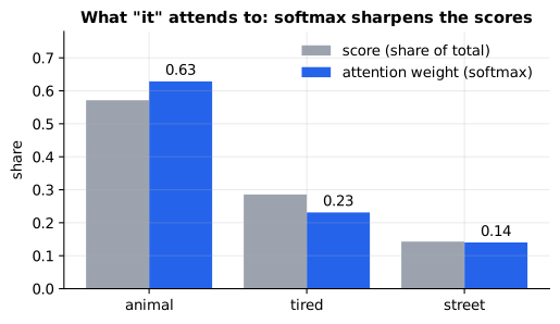
Reading it: for each word, the grey bar is its share of the raw scores and the blue bar is its share of attention after softmax. Softmax exaggerates differences: "animal" scores only twice as high as "tired", yet it ends up with almost three times the attention, because exponentiating stretches the gaps. That is how attention commits to the most relevant word while keeping a little of the others.
In code: softmax subtracts the largest score before exponentiating, and turns masked scores of −∞ into weights of exactly 0.
Where the scores come from: queries, keys and values
Each word turns its vector into three new vectors by multiplying it by three learned matrices:
- a query: what am I looking for? ("it" is looking for a noun that can be tired.)
- a key: what do I offer to others? ("animal" offers: a noun, alive.)
- a value: what I actually hand over if someone picks me.
A word's score for another word is the dot product of its query with the other word's key: multiply them position by position and add.
Level 3: the formula and its symbols
$$ q \cdot k = \sum_{m=1}^{d_k} q_m \, k_m $$
Symbols
| Symbol | Meaning here | In the example |
|---|---|---|
| $q$ | the query vector: a list of $d_k$ numbers | (1, 2) |
| $k$ | the key vector: another list of $d_k$ numbers | (3, 0.5) |
| $d_k$ | how many numbers each list has (the head width) | 2 |
| $m$ | a counter walking over the positions | 1, 2 |
| $q_m, k_m$ | the $m$-th number in each list | $q_1 = 1$, $k_1 = 3$ |
| $\cdot$ | "dot product": multiply matching positions, then add |
In words: "multiply the first numbers together, multiply the second numbers together, and so on, then add up all the products."
With the numbers: (1, 2) · (3, 0.5) = 1·3 + 2·0.5 = 3 + 1 = 4.
Level 3: in Python
In Python:
q = [1, 2]
k = [3, 0.5]
# Σ over m of q_m k_m
sum(q_m * k_m for q_m, k_m in zip(q, k))  # → 4.0
Vectors that point the same way give big positive scores, vectors at right angles give zero, and opposite vectors give negative scores. That is why the dot product works as a relevance score. The values are then blended with the softmax shares, exactly as in the table above.
A library search is a good analogy. The query is what you type into the search box, the keys are the catalogue entries, and the values are the books on the shelf. You get back a blend of books, weighted by how well each catalogue entry matched your search.
flowchart LR
  X[Token vectors] --> Q[Query] & K[Key] & V[Value]
  Q --> S[Scores<br/>Q times K]
  K --> S
  S --> SC[Scale by<br/>sqrt of d_k]
  SC --> M[Causal mask<br/>hide future tokens]
  M --> SM[Softmax<br/>weights sum to 1]
  SM --> W[Weighted sum<br/>of values]
  V --> W
  W --> O[Context-aware vectors]
Reading it: follow the arrows left to right. The token vectors split three ways. Queries and keys meet in the Scores box: that is where relevance is decided. The values take the lower path and wait, untouched, until the Weighted sum box, where the relevance shares decide how much of each value is mixed in. Keep the two roles apart: Q and K decide how much; V carries what. The Scale and Mask boxes are explained in their own sections below.
Written as one formula, with every word's query stacked into a matrix Q (and likewise K and V), the whole diagram is:
Level 3: the formula and its symbols
$$ \text{Attention}(Q, K, V) = \text{softmax}\left(\frac{QK^\top}{\sqrt{d_k}}\right)V $$
Symbols
| Symbol | Meaning here | Shape |
|---|---|---|
| $n$ | number of tokens in the sequence | |
| $d_k$ | width of each query and key vector | |
| $d_v$ | width of each value vector | |
| $Q$ | every token's query, stacked as rows | $n \times d_k$ |
| $K$ | every token's key, stacked as rows | $n \times d_k$ |
| $V$ | every token's value, stacked as rows | $n \times d_v$ |
| $K^\top$ | $K$ transposed: rows become columns, so each key stands upright | $d_k \times n$ |
| $QK^\top$ | a matrix multiply: entry (row $i$, column $j$) is the dot product of token $i$'s query with token $j$'s key, so it is every score at once | $n \times n$ |
| $\sqrt{d_k}$ | square root of the head width; dividing by it keeps scores from growing with width (explained below) | a single number |
| softmax(…) | softmax applied to each row separately, so each token's shares add to 1 | $n \times n$ |
| $(\ldots)V$ | multiply the shares by the values: each output row is a share-weighted blend of value rows | $n \times d_v$ |
In words: "score every query against every key, shrink the scores by √d_k, turn each row of scores into shares, and use the shares to blend the values."
With the numbers: the "it" row of $QK^\top/\sqrt{d_k}$ holds (2.0, 1.0, 0.5); softmax turns that row into (0.63, 0.23, 0.14); multiplying by $V$ gives 0.63·V(animal) + 0.23·V(tired) + 0.14·V(street). To see every symbol at work, take $d_k = 4$: the query of "it" (1, 1, 1, 1) against the keys (1, 1, 1, 1), (1, 1, 0, 0) and (1, 0, 0, 0) gives raw scores (4, 2, 1), and dividing by $\sqrt{4} = 2$ gives exactly that row. With toy values V(animal) = (1, 0), V(tired) = (0, 1) and V(street) = (1, 1), the blend is (0.63 + 0.14, 0.23 + 0.14) = (0.77, 0.37).
Level 3: in Python
In Python:
import math
q_it = [1, 1, 1, 1]
# keys: animal, tired, street
K = [[1, 1, 1, 1], [1, 1, 0, 0], [1, 0, 0, 0]]
# values, one row per word
V = [[1, 0], [0, 1], [1, 1]]
d_k = len(q_it)
# q Kᵀ / √d_k
scores = [sum(q * k for q, k in zip(q_it, k_j)) / math.sqrt(d_k) for k_j in K]
scores  # → [2.0, 1.0, 0.5]
exps = [math.exp(s) for s in scores]
# softmax of the row
weights = [e / sum(exps) for e in exps]
[round(w, 2) for w in weights]  # → [0.63, 0.23, 0.14]
# (…)V: blend the values
[round(sum(w * v[c] for w, v in zip(weights, V)), 2) for c in range(2)]  # → [0.77, 0.37]
In practice this one line runs in every layer of every modern language model, for every word, many times per word generated. Nearly everything about a model's speed and memory use traces back to it.
In code: scaled_dot_product_attention is the whole formula, one commented step per box of the diagram, and returns both the blended values and the attention weights.
Shapes: the part that is easiest to get wrong
For one sequence of n tokens with model width d_model:
| Tensor | Shape | Meaning |
|---|---|---|
| X | (n, d_model) | input token vectors |
| W_q, W_k | (d_model, d_k) | learned projections |
| W_v | (d_model, d_v) | learned projection |
| Q, K | (n, d_k) | queries, keys |
| V | (n, d_v) | values |
| Q Kᵀ | (n, n) | every token vs. every token, hence O(n²) |
| weights | (n, n) | each row sums to 1 |
| output | (n, d_v) | one context-aware vector per token |
Causal masking: no peeking at the answer
A decoder model (GPT, Claude, Llama) is trained to predict the next token. If position i could attend to position i+1, it could simply read the answer. So the scores for future positions are set to −∞ before softmax. Because e^−∞ = 0, those weights come out as exactly zero.
flowchart LR
  subgraph S["Scores (n × n)"]
    direction TB
    r0["row 'The':    ✓ · · ·"]
    r1["row 'cat':    ✓ ✓ · ·"]
    r2["row 'sat':    ✓ ✓ ✓ ·"]
    r3["row 'down':   ✓ ✓ ✓ ✓"]
  end
  S --> MASK["set every · to −∞"] --> SOFT["softmax per row"] --> OUT["each row sums to 1<br/>using only the past"]
Reading it: each row is one token looking at the sequence. A ✓ is a position it may read and a · is the future, which gets masked. The allowed region is a lower triangle: the first token sees only itself and the last sees everything before it. The same triangle appears as the dark region in the heatmap below.
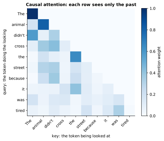
Reading it: rows are the token doing the looking (the query), columns are the tokens being looked at (the keys), and darker means more weight. The upper-right triangle is exactly zero, so nothing reads the future. Each row sums to 1, so a token's attention is a budget it spends across the past. The weights come from random projections here, so the pattern itself means nothing; the triangle is what matters. In a trained model, rows light up on the tokens that actually help, such as "it" lighting up "animal".
Try it: here is the same sentence with hand-picked queries and keys, so the pattern does mean something; "it" keeps the worked example's scores for "animal", "tired" and "street". Pick the row for "it", then turn the causal mask on: "tired" comes later, so its weight drops to exactly 0 and "animal" takes a bigger share. Drag the temperature below 1 to watch each row sharpen towards one word, and above 1 to watch it flatten towards an even spread.
Masking only the future is also what makes generation cheap: a token's
output never changes when later tokens arrive, so it can be computed once
and cached. See primer.ml.inference for the KV cache.
In code: causal_mask builds the lower triangle of allowed positions, and scaled_dot_product_attention sets every score outside it to −∞ before softmax. worked_example_sentence holds the hand-picked queries and keys the heatmap above draws.
Why divide by √d_k?
Everyday picture. Roll one die and the result swings between 1 and 6. Add up a hundred dice and the total swings far more, by dozens in either direction. A dot product is exactly that kind of sum: one small random-ish product per position. The wider the vectors, the more terms get added, and the wilder the scores swing.
Tiny example. With d_k = 4, a query and a key of random ±1 entries give four products of +1 or −1, so the score lands between −4 and +4 and is usually within ±2. With d_k = 256 it's a sum of 256 such products: usually within ±16. Softmax of scores like (16, 3, −9) gives about (0.999998, …, …). All the attention lands on one word, whether or not that is right.
Level 3: the formula and its symbols
$$ \operatorname{Var}(q \cdot k) = d_k \qquad\Longrightarrow\qquad \operatorname{Var}!\left(\frac{q \cdot k}{\sqrt{d_k}}\right) = 1 $$
Symbols
| Symbol | Meaning here |
|---|---|
| $\operatorname{Var}(x)$ | variance: the average squared distance of $x$ from its average; a measure of how widely $x$ swings. Its square root is the standard deviation, the typical size of a swing |
| $q \cdot k$ | a raw attention score, for $q$ and $k$ whose entries are independent with average 0 and variance 1 |
| $d_k$ | the number of products added up in the dot product |
| $\Longrightarrow$ | "which implies" |
| $\sqrt{d_k}$ | dividing a quantity by $c$ divides its variance by $c^2$; here $c^2 = d_k$ |
In words: "the spread of a raw score grows with the head width, so we divide the score by the square root of the width, which brings the spread back to 1 at any width."
With the numbers: at d_k = 128, the standard deviation of a raw score is √128 ≈ 11.3, so scores of ±20 are routine. After dividing by √128 the standard deviation is 1, so scores of ±2 are typical. At d_k = 4 you can check the formula exactly: the 16 equally likely patterns of four ±1 products give raw scores whose variance is 4, and dividing each by √4 = 2 brings the variance to 1.
Level 3: in Python
In Python:
import itertools, math, statistics
d_k = 4
scores = [sum(products) for products in itertools.product([-1, 1], repeat=d_k)]
# Var(q · k) = d_k
statistics.pvariance(scores)  # → 4
# Var(q · k / √d_k) = 1
statistics.pvariance([s / math.sqrt(d_k) for s in scores])  # → 1.0
# the typical raw swing at d_k = 128
round(math.sqrt(128), 1)  # → 11.3
Why "all attention on one word" is bad, beyond being a wrong answer: softmax
has stopped responding. Its gradient (the signal training uses to
adjust the weights) is diag(p) − p pᵀ, and when one share is 1 and the rest
are 0, every entry of that matrix is 0. The query and key weights receive no
signal and stop learning. This is called saturation.
sqrt_dk_experiment measures all of this.
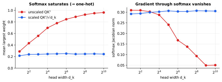
Reading it: the x-axis is the head width d_k, on a log scale. On the left, the y-axis is the average largest attention weight: 1.0 means one-hot, all attention on one token. On the right, it is the size of the softmax gradient. The unscaled lines (red) climb towards 1.0 on the left and fall towards zero on the right as d_k grows: the wider the head, the more attention collapses onto a single token and the less signal flows back. The scaled lines (blue) stay flat at every width. That flatness is the whole reason for the √d_k.
In one sentence: dot products grow with dimension, large scores saturate softmax and kill gradients, and scaling by √d_k keeps scores in the range where softmax is smooth and trainable.
In code: softmax_jacobian builds the diag(p) − p pᵀ matrix, so you can watch every entry fall to 0 as one share approaches 1.
Multi-head attention
Instead of one attention with d_k = d_model, run h heads in parallel, each with d_k = d_model / h and its own W_q, W_k and W_v. The total compute is the same, but each head can specialise: one tracks syntax, another which noun a pronoun refers to, another the previous token.
flowchart LR
  X["X (n × d_model)"] --> P["project with W_q, W_k, W_v"]
  P --> H1["head 1<br/>attention on d_model/h dims"]
  P --> H2["head 2"]
  P --> H3["..."]
  P --> Hh["head h"]
  H1 & H2 & H3 & Hh --> C["concatenate<br/>(n × d_model)"]
  C --> WO["mix with W_o"] --> Y["output (n × d_model)"]
Reading it: the input is projected once, and the result is sliced into h narrow slabs, one per head. Each head runs the full attention recipe from the first diagram on its own slab, independently and in parallel. The heads' outputs are glued back side by side, and W_o lets them exchange what they found. The output has the same shape as the input, which is what lets blocks stack.
In code: MultiHeadAttention holds the four projections W_q, W_k, W_v and W_o; calling it slices the projections into one slab per head, runs scaled_dot_product_attention on every head at once, and glues the results back together before W_o.
Grouped-query attention: sharing keys and values
With grouped-query attention (GQA), several query heads share one key/value head. Llama 3 8B has 32 query heads but only 8 KV heads, so it stores 4× fewer keys and values per token. Multi-query attention (MQA) is the extreme: one KV head for everyone.
flowchart TB
  subgraph MHA["MHA: 4 query heads, 4 KV heads"]
    q1a[Q1]-->kv1a[KV1]
    q2a[Q2]-->kv2a[KV2]
    q3a[Q3]-->kv3a[KV3]
    q4a[Q4]-->kv4a[KV4]
  end
  subgraph GQA["GQA: 4 query heads, 2 KV heads"]
    q1b[Q1]-->kv1b[KV1]
    q2b[Q2]-->kv1b
    q3b[Q3]-->kv2b[KV2]
    q4b[Q4]-->kv2b
  end
  subgraph MQA["MQA: 4 query heads, 1 KV head"]
    q1c[Q1]-->kv1c[KV1]
    q2c[Q2]-->kv1c
    q3c[Q3]-->kv1c
    q4c[Q4]-->kv1c
  end
Reading it: count the KV boxes. Every query head still asks its own
question, but in GQA and MQA they read from a shared set of keys and values.
The KV boxes are what gets stored in GPU memory for every token of every
conversation during generation (the KV cache). Fewer boxes means more
conversations fit on one GPU, at a small cost in quality. See
primer.ml.inference for the memory arithmetic.
In code: MultiHeadAttention takes a number of KV heads: fewer than the query heads is GQA, one is MQA. MultiHeadAttention.kv_params counts the key and value weights that shrink.
Cost: why long context is expensive
The score matrix is n × n per head per layer, so compute and memory grow with n². Doubling the context roughly quadruples attention's cost.
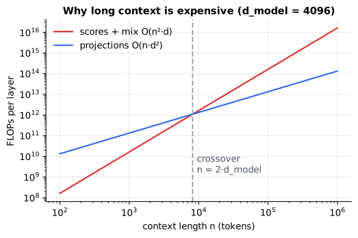
Reading it: both axes are logarithmic, so a straight line is a power law and a steeper line grows faster. The projections (X·W) cost O(n·d²), a line of slope 1. The score-and-mix step costs O(n²·d), a line of slope 2. The dashed marker is where they cross, at n = 2·d_model. Past that point, most of the work is tokens comparing themselves to other tokens, and every doubling of context costs 4× there.
The standard mitigations each attack this picture. FlashAttention produces the exact same result but computes it in tiles sized for fast on-chip GPU memory, so the n × n matrix is never written to slow memory. Sliding-window and sparse attention let each token see only some others. GQA and MQA shrink the KV cache. State-space models such as Mamba replace attention with a linear-time recurrence.
In code: attention_cost counts the quadratic score-and-mix FLOPs and the linear projection FLOPs plotted above.
In 20 seconds
- Attention: each token builds a query, key and value. Query-key similarity decides how much each token listens to each other token, and the output is a weighted blend of their values.
- Why √d_k: dot products grow with dimension, and large scores saturate softmax and kill gradients. Scaling keeps training stable.
- Causal mask: future scores are set to −∞ before softmax, so each token sees only the past. That is what makes next-token training honest and generation cacheable.
- Long context cost: attention compares every pair of tokens, so it is O(n²), and the KV cache grows with every token.
Self-test questions
Explain attention to a non-engineer in 30 seconds. When the model reads a word, it asks which other words here help it understand this one. It scores every other word for relevance, then builds its understanding of the word as a mix of the relevant ones. In "the animal didn't cross the street because it was tired", "it" draws mostly from "animal". It does this for every word, in parallel, dozens of times over.
Now explain it to an ML engineer in two minutes. Project X into Q, K and V with learned matrices. Compute QKᵀ/√d_k, an n×n matrix of scaled similarities; add a causal mask of −∞ above the diagonal for a decoder; softmax each row; multiply by V. Run h heads in parallel on d_model/h slices, concatenate them, and project with W_o. Wrap the whole thing in a residual connection with pre-layer-norm and follow it with an FFN. Cost is O(n²·d) in compute and O(n²) in memory for the scores, which is why FlashAttention tiles it and GQA shrinks the KV cache.
Why divide by √d_k? What breaks without it? The variance of q·k grows linearly with d_k. Without scaling, scores spread out, softmax saturates towards one-hot, its Jacobian goes to about zero, and the query/key projections stop receiving gradient. Training stalls or turns unstable.
Why is long context expensive? Name two techniques that reduce the cost. Scores are n×n per head per layer, so cost is quadratic, and the KV cache grows linearly with every token held in memory. Two fixes: FlashAttention (exact, memory-efficient tiling) and GQA/MQA (fewer KV heads). Others: sliding-window or sparse attention, and prompt caching of stable prefixes.
What does the causal mask buy you besides honest training? Earlier outputs never depend on later tokens, so during generation the keys and values of past tokens can be computed once and cached. Each new token then costs one row of attention instead of a full recomputation.
What does GQA trade away, and for what? A little modelling capacity (query heads share keys and values) for a KV cache that is several times smaller. That means more concurrent requests and longer contexts per GPU.
The papers behind this lesson
- Vaswani et al., Attention Is All You Need (2017): https://arxiv.org/abs/1706.03762. Showed that attention alone, with no recurrence, is enough for state-of-the-art translation, and introduced scaled dot-product attention, multi-head attention and the transformer. Annotated companion
- Ainslie et al., GQA: Training Generalized Multi-Query Transformer Models from Multi-Head Checkpoints (2023): https://arxiv.org/abs/2305.13245. Introduced grouped-query attention, the middle ground between multi-head and multi-query attention.
- Dao et al., FlashAttention (2022): https://arxiv.org/abs/2205.14135. Computes exact attention in tiles sized for fast on-chip GPU memory, making long contexts practical. Annotated companion
Further reading
- Vaswani et al., Attention Is All You Need (2017): https://arxiv.org/abs/1706.03762
- Jay Alammar, The Illustrated Transformer: https://jalammar.github.io/illustrated-transformer/
- Harvard NLP, The Annotated Transformer (the paper, line by line in code): https://nlp.seas.harvard.edu/annotated-transformer/
- Andrej Karpathy, Let's build GPT: from scratch, in code, spelled out: https://www.youtube.com/watch?v=kCc8FmEb1nY and nanoGPT: https://github.com/karpathy/nanoGPT
- 3Blue1Brown, Attention in transformers, visually explained: https://www.youtube.com/watch?v=eMlx5fFNoYc
- PyTorch
scaled_dot_product_attention: https://pytorch.org/docs/stable/generated/torch.nn.functional.scaled_dot_product_attention.html - Ainslie et al., GQA (2023): https://arxiv.org/abs/2305.13245
- Dao et al., FlashAttention (2022): https://arxiv.org/abs/2205.14135
1r""" 2# Attention: how a token decides what to listen to 3 4Run: `python -m primer.ml.attention` 5 6New to the notation? `primer.notation` explains every symbol used here from 7zero. This lesson builds on the vectors and matrix multiplies of 8`primer.ml.neural_net`. 9 10## Level 1: The practitioner's guide 11 12**In one sentence.** Attention is the step in which every token of a 13model's input scores every other token for relevance and rebuilds itself as 14a weighted blend of the ones that matter; because the comparison is 15all-pairs, it sets a model's context limit, the price of a long prompt, and 16the memory a conversation occupies on a GPU. 17 18**When you need it.** You never switch attention on: every transformer you 19call already runs it in every layer. You need to understand it the day a 20decision turns on its cost: picking a model by its context window or by the 21key-value heads on its model card, deciding whether to put 200 pages in one 22prompt or retrieve the relevant three, sizing a GPU for a model you host, or 23explaining why a call with a long history is slow before the first output 24token appears. The tell: latency and cost that grow with the length of the 25conversation rather than the length of the answer. From this lesson's 26`attention_cost`: a 1,000-token prompt builds a score 27matrix of 1,000,000 entries per head per layer, a 2,000-token prompt 284,000,000, and a 128,000-token prompt 16.4 billion. Doubling the context 29quadruples that part of the work. Below a few thousand tokens you can 30ignore it: the parts of the model that grow linearly dominate (the lesson's 31crossover is at twice the model width, 8,192 tokens for a 4,096-wide model). 32 33**Your options.** Some of these you choose in your prompt or API call; the 34rest you choose by picking a model or a serving stack. From the cheapest to 35the most committed: 36 37| Option | What it does | What it gives you | What it costs | Where it lives | 38|---|---|---|---|---| 39| Short prompts, retrieval for the rest | Puts only the relevant text in the context | Cost that stays flat as the corpus grows | An index to build and a retrieval step that can miss | Your code (`primer.agents.rag`) | 40| Prompt caching | Reuses the keys and values of a prefix that repeats across calls | Cache reads at 0.1× the input price and a faster first token | The prefix must be identical byte for byte; a cache write costs 1.25× | The API, or the serving engine | 41| A long context window | Sends the whole document or history in one call | Nothing to retrieve; exact cross-references over all of it | Quadratic compute, a cache that grows with every token, weaker recall in the middle | The model you pick: up to 1M tokens on current hosted models | 42| A GQA or MQA model | Shares each key-value head among several query heads | A KV cache 4× to 8× smaller, so more conversations fit on one GPU | A small loss of modelling capacity, decided by the model's authors | The model card: `num_key_value_heads` | 43| FlashAttention kernels | Computes the same attention in tiles that stay in fast on-chip memory | The exact result, 2× to 3× faster, and no n × n matrix in slow memory | A supported GPU; nothing to tune | The serving stack: PyTorch, vLLM and the rest | 44| Sliding-window attention | Lets each layer look back a fixed number of tokens | A cache of fixed size per token and linear cost at any length | Exact lookup beyond the window is gone; information hops layer by layer | The model architecture (Mistral 7B: a 4,096-token window) | 45| A paged KV cache | Stores each request's cache in small blocks instead of one reserved strip | 2× to 4× the throughput from the same GPU memory | A serving engine that supports it | vLLM, and most engines since | 46| A linear-time architecture | Replaces attention with a recurrence that carries a fixed-size state | No n² term and a cache that does not grow | Different recall behaviour and fewer mature models | The model architecture (state-space models such as Mamba) | 47 48**How to choose.** Start from what you control. 49 50- A hosted API: you control the prompt. Put the stable part (system prompt, 51 tool definitions, reference documents) first and keep it identical so it 52 caches; put what changes last. Count tokens before you send: input that 53 exceeds the window is rejected, not truncated. 54- Long context or retrieval: long context for one document the model must 55 read exactly (a contract, a codebase), retrieval when the corpus outlives 56 a single prompt or the relevant part is small. Most production systems do 57 both: retrieve, then give the model a generous window of what came back. 58- An open model to host: read `num_attention_heads`, `num_key_value_heads` 59 and `max_position_embeddings` on its card. The cache per token scales with 60 the key-value heads, and that number, not the parameter count, decides how 61 many conversations one GPU carries. 62- Serving it: use an engine that ships FlashAttention and paged caching 63 rather than a loop of your own. 64- Training or fine-tuning: keep the library's score scaling and causal mask 65 as they are; Level 2 measures what happens without them. 66- Whatever you pick, measure quality against context length on your own 67 task, with the answer placed at the start, the middle and the end. A 68 longer advertised window does not make a model better at using the middle 69 of it. 70 71**What it costs.** Four currencies: compute, memory, money and recall. 72 73- Compute. The score-and-mix step is quadratic in tokens and is paid in full 74 when a prompt is first read: that is the pause before the first output 75 token. From `attention_cost` with a 4,096-wide model, at 8,000 tokens the 76 quadratic part equals the linear part; at 128,000 tokens it is about 16 77 times larger. 78- Memory. Every token of every live conversation keeps its keys and values 79 in the KV cache. For a Llama-3-8B-shaped model (32 layers, 8 key-value 80 heads of width 128, 16-bit numbers) that is 131,072 bytes per token, so a 81 32,000-token conversation holds about 4.2 GB, and an 80 GB GPU with 16 GB 82 of weights carries 15 such conversations. At 128,000 tokens, 32 key-value 83 heads would need 67 GB for one request; 8 need 17 GB. The figures are 84 `primer.ml.inference`'s. 85- Money. Hosted APIs bill per token at a flat rate across the window: a 86 100,000-token prompt on a model priced at \$5 per million input tokens 87 costs \$0.50 each time it is sent, and \$0.05 when the whole prompt is a 88 cache read at 0.1×. A 900,000-token request costs the same per token as a 89 9,000-token one (Anthropic's pricing page): the quadratic compute is 90 priced into the flat rate. 91- Recall. In the Lost in the Middle study (Liu et al., 2023), GPT-3.5-Turbo 92 answered 75.8% of questions when the useful document was first among 20 93 and 53.8% when it was tenth, below its 56.1% with no documents at all. 94 95**What breaks.** 96 97- **The answer in the middle.** Accuracy falls when the relevant text sits 98 mid-prompt. Put the most important material first or last, and keep 99 prompts as short as the task allows. 100- **A cache that never hits.** A timestamp or request id near the top of 101 the prompt changes the prefix on every call, and every call pays full 102 price. If the cache-read count in the usage report is zero across 103 identical requests, something volatile sits before the stable part. 104- **Out of memory at long context.** The KV cache, not the weights, is what 105 overflows a GPU on long requests. Prefer a GQA model, cap the context you 106 accept, or run an engine that pages the cache. 107- **A prompt that does not fit.** Input beyond the window is an error; input 108 plus the output budget beyond it stops generation early. Count tokens 109 first and leave room for the answer. 110- **Training instability from unscaled scores.** Without the division by 111 the square root of the head width, this lesson's measurement at width 512 112 puts 0.94 of the attention on one token on average and shrinks the 113 training signal fivefold; the model stops learning what to attend to. 114 115**In the wild.** The original transformer (Vaswani et al., 2017) ran 8 heads 116of width 64 on 512-wide vectors. Anthropic's context-window documentation gives current models a 1M-token 117window and counts everything in the request towards it: system prompt, tool 118definitions, tool results and the model's own thinking. Hugging Face model 119configs expose `num_attention_heads`, `num_key_value_heads` and 120`max_position_embeddings`; Llama 3 pairs 32 query heads with 8 key-value 121heads and reaches 128K tokens, and Mistral 7B uses the same 32-to-8 split 122plus a 4,096-token sliding window whose reach grows to about 131K tokens 123across its 32 layers. The GQA paper converted multi-head checkpoints with 5% 124of the original pretraining compute. PyTorch's 125`scaled_dot_product_attention` chooses among a FlashAttention-2 kernel, a 126memory-efficient kernel and a plain implementation by itself, and vLLM's 127PagedAttention lifted serving throughput 2 to 4 times over earlier engines, 128whose reserved-strip caches held real tokens in only 20% to 38% of their 129memory. The papers are linked at the end of the lesson. 130 131**Go deeper.** Level 2 builds attention from three numbers: softmax on a 132pronoun's scores, queries, keys and values on a four-number example, the 133causal mask that makes caching possible, the square-root scaling measured at 134three widths, multi-head and grouped-query attention in a class you can 135call, and the n² curve. If you only needed to choose a model or shape a 136prompt, you are done. 137 138## Level 2: How it works, from scratch 139 140Level 2 builds the mechanism from nothing, starting with a glance around a 141room. 142 143**The everyday picture.** Imagine you're in a meeting and someone says "it's broken, can you fix it?" 144To know what "it" means, you glance around the room: at the laptop on the 145table, at the person who just walked in, at the whiteboard. You pay a lot of 146attention to the laptop, a little to everything else, and your understanding 147of "it" becomes mostly *laptop*. 148 149That glance is attention. Every word in a sentence gets to look at every 150other word, decide how relevant each one is, and rebuild its own meaning as 151a mix of the relevant ones. "Bank" next to "river" becomes a riverbank; next 152to "loan" it becomes a lender. The word is the same, but what it paid 153attention to is different. 154 155## A tiny worked example: what does "it" refer to? 156 157Take "The animal didn't cross the street because it was tired" and follow 158the word "it". To keep the numbers small, it compares itself with just three 159other words. Each comparison gives a relevance **score** (how the score is 160made comes next). Then we turn scores into shares of attention that add up 161to 1: 162 1631. Exponentiate each score (e^score), which makes every number positive and 164 stretches the gaps between them. 1652. Divide each by the total, 7.39 + 2.72 + 1.65 = 11.76. 166 167| Word | Score | e^score | Share of attention | 168|--------|-------|---------|--------------------| 169| animal | 2.0 | 7.39 | 7.39 / 11.76 = **0.63** | 170| tired | 1.0 | 2.72 | 2.72 / 11.76 = **0.23** | 171| street | 0.5 | 1.65 | 1.65 / 11.76 = **0.14** | 172 173Those two steps are called **softmax**. The new meaning of "it" is 63% 174"animal", 23% "tired" and 14% "street". Without being told any grammar rule, 175the model has worked out that "it" is the animal. 176 177**In code:** `worked_example_it` runs these three scores through softmax and returns each word's share. 178 179### Softmax, decoded 180 181Softmax turns any list of numbers, positive or negative, into shares that 182are all positive and add up to exactly 1. Think of it as a vote where louder 183voices get disproportionately more say. 184 185$$ 186\text{softmax}(z)_i = \frac{e^{z_i}}{\sum_{j=1}^{n} e^{z_j}} 187$$ 188 189**Symbols** 190 191| Symbol | Meaning here | In the example | 192|---|---|---| 193| $z$ | the list of scores going in | (2.0, 1.0, 0.5) | 194| $n$ | how many scores there are | 3 | 195| $i$ | the position we're computing a share for | 1 = "animal" | 196| $z_i$ | the score at position $i$ | $z_1 = 2.0$ | 197| $e$ | Euler's number, ≈ 2.718; $e^x$ is "2.718 multiplied by itself $x$ times" (works for fractions and negatives too) | $e^{2.0} = 7.39$ | 198| $\sum_{j=1}^{n}$ | "add up the following, for $j$ = 1, 2, …, $n$" | $e^{2.0} + e^{1.0} + e^{0.5}$ | 199| $j$ | a counter that walks over every position | 1, 2, 3 | 200| $\text{softmax}(z)_i$ | the share of attention position $i$ gets | 0.63 | 201 202**In words:** "the share for item *i* is *e* raised to its score, divided by 203the sum of *e* raised to every score." 204 205**With the numbers:** softmax(2.0, 1.0, 0.5)₁ = 7.39 / (7.39 + 2.72 + 1.65) = 2067.39 / 11.76 = 0.63. 207 208**In Python:** 209 210```python 211import math 212# animal, tired, street 213z = [2.0, 1.0, 0.5] 214# e^(z_i) for each score 215exps = [math.exp(z_i) for z_i in z] 216[round(e, 2) for e in exps] # → [7.39, 2.72, 1.65] 217# Σ_j e^(z_j) 218total = sum(exps) 219round(total, 2) # → 11.76 220# softmax(z)_i: each share of the total 221[round(e / total, 2) for e in exps] # → [0.63, 0.23, 0.14] 222``` 223 224Why *e* to the power of the score, and not just the score divided by the 225total? Three reasons you can check on the table above: 226 2271. **Always positive.** Scores can be negative; *e* to any power is positive, 228 so no word ever gets a negative share. 2292. **Order is kept.** A higher score always gets a bigger share. 2303. **Gaps are stretched.** Adding 1 to a score multiplies its *e*-value by 231 2.72, so the winner pulls ahead decisively. (Plain division would give 232 "animal" 2.0 / 3.5 = 0.57, a timid 57%, and would break on negative 233 scores.) 234 235One more property matters later: adding the same number to every score 236changes nothing, because it multiplies the top and bottom of the fraction by 237the same amount. The code uses this to subtract the largest score before 238exponentiating, which stops *e*¹⁰⁰⁰ from overflowing to infinity. See 239`primer.notation` for exponents and sums from scratch. 240 241 242 243**Reading it:** for each word, the grey bar is its share of the raw scores 244and the blue bar is its share of attention after softmax. Softmax exaggerates 245differences: "animal" scores only twice as high as "tired", yet it ends up 246with almost three times the attention, because exponentiating stretches the 247gaps. That is how attention commits to the most relevant word while keeping 248a little of the others. 249 250**In code:** `softmax` subtracts the largest score before exponentiating, and turns masked scores of −∞ into weights of exactly 0. 251 252## Where the scores come from: queries, keys and values 253 254Each word turns its vector into three new vectors by multiplying it by three 255learned matrices: 256 257- a **query**: what am I looking for? ("it" is looking for a noun that can 258 be tired.) 259- a **key**: what do I offer to others? ("animal" offers: a noun, alive.) 260- a **value**: what I actually hand over if someone picks me. 261 262A word's score for another word is the **dot product** of its query with the 263other word's key: multiply them position by position and add. 264 265$$ 266q \cdot k = \sum_{m=1}^{d_k} q_m \, k_m 267$$ 268 269**Symbols** 270 271| Symbol | Meaning here | In the example | 272|---|---|---| 273| $q$ | the query vector: a list of $d_k$ numbers | (1, 2) | 274| $k$ | the key vector: another list of $d_k$ numbers | (3, 0.5) | 275| $d_k$ | how many numbers each list has (the head width) | 2 | 276| $m$ | a counter walking over the positions | 1, 2 | 277| $q_m, k_m$ | the $m$-th number in each list | $q_1 = 1$, $k_1 = 3$ | 278| $\cdot$ | "dot product": multiply matching positions, then add | | 279 280**In words:** "multiply the first numbers together, multiply the second 281numbers together, and so on, then add up all the products." 282 283**With the numbers:** (1, 2) · (3, 0.5) = 1·3 + 2·0.5 = 3 + 1 = **4**. 284 285**In Python:** 286 287```python 288q = [1, 2] 289k = [3, 0.5] 290# Σ over m of q_m k_m 291sum(q_m * k_m for q_m, k_m in zip(q, k)) # → 4.0 292``` 293 294Vectors that point the same way give big positive scores, vectors at right 295angles give zero, and opposite vectors give negative scores. That is why the 296dot product works as a relevance score. The values are then blended with 297the softmax shares, exactly as in the table above. 298 299A library search is a good analogy. The query is what you type into the 300search box, the keys are the catalogue entries, and the values are the books 301on the shelf. You get back a *blend* of books, weighted by how well each 302catalogue entry matched your search. 303 304```mermaid 305flowchart LR 306 X[Token vectors] --> Q[Query] & K[Key] & V[Value] 307 Q --> S[Scores<br/>Q times K] 308 K --> S 309 S --> SC[Scale by<br/>sqrt of d_k] 310 SC --> M[Causal mask<br/>hide future tokens] 311 M --> SM[Softmax<br/>weights sum to 1] 312 SM --> W[Weighted sum<br/>of values] 313 V --> W 314 W --> O[Context-aware vectors] 315``` 316 317**Reading it:** follow the arrows left to right. The token vectors split 318three ways. Queries and keys meet in the Scores box: that is where relevance 319is decided. The values take the lower path and wait, untouched, until the 320Weighted sum box, where the relevance shares decide how much of each value 321is mixed in. Keep the two roles apart: **Q and K decide *how much*; V carries 322*what*.** The Scale and Mask boxes are explained in their own sections below. 323 324Written as one formula, with every word's query stacked into a matrix Q (and 325likewise K and V), the whole diagram is: 326 327$$ 328\text{Attention}(Q, K, V) = \text{softmax}\left(\frac{QK^\top}{\sqrt{d_k}}\right)V 329$$ 330 331**Symbols** 332 333| Symbol | Meaning here | Shape | 334|---|---|---| 335| $n$ | number of tokens in the sequence | | 336| $d_k$ | width of each query and key vector | | 337| $d_v$ | width of each value vector | | 338| $Q$ | every token's query, stacked as rows | $n \times d_k$ | 339| $K$ | every token's key, stacked as rows | $n \times d_k$ | 340| $V$ | every token's value, stacked as rows | $n \times d_v$ | 341| $K^\top$ | $K$ **transposed**: rows become columns, so each key stands upright | $d_k \times n$ | 342| $QK^\top$ | a **matrix multiply**: entry (row $i$, column $j$) is the dot product of token $i$'s query with token $j$'s key, so it is every score at once | $n \times n$ | 343| $\sqrt{d_k}$ | square root of the head width; dividing by it keeps scores from growing with width (explained below) | a single number | 344| softmax(…) | softmax applied to each row separately, so each token's shares add to 1 | $n \times n$ | 345| $(\ldots)V$ | multiply the shares by the values: each output row is a share-weighted blend of value rows | $n \times d_v$ | 346 347**In words:** "score every query against every key, shrink the scores by √d_k, 348turn each row of scores into shares, and use the shares to blend the values." 349 350**With the numbers:** the "it" row of $QK^\top/\sqrt{d_k}$ holds (2.0, 1.0, 3510.5); softmax turns that row into (0.63, 0.23, 0.14); multiplying by $V$ 352gives 0.63·V(animal) + 0.23·V(tired) + 0.14·V(street). To see every symbol 353at work, take $d_k = 4$: the query of "it" (1, 1, 1, 1) against the keys 354(1, 1, 1, 1), (1, 1, 0, 0) and (1, 0, 0, 0) gives raw scores (4, 2, 1), and 355dividing by $\sqrt{4} = 2$ gives exactly that row. With toy values 356V(animal) = (1, 0), V(tired) = (0, 1) and V(street) = (1, 1), the blend is 357(0.63 + 0.14, 0.23 + 0.14) = (0.77, 0.37). 358 359**In Python:** 360 361```python 362import math 363q_it = [1, 1, 1, 1] 364# keys: animal, tired, street 365K = [[1, 1, 1, 1], [1, 1, 0, 0], [1, 0, 0, 0]] 366# values, one row per word 367V = [[1, 0], [0, 1], [1, 1]] 368d_k = len(q_it) 369# q Kᵀ / √d_k 370scores = [sum(q * k for q, k in zip(q_it, k_j)) / math.sqrt(d_k) for k_j in K] 371scores # → [2.0, 1.0, 0.5] 372exps = [math.exp(s) for s in scores] 373# softmax of the row 374weights = [e / sum(exps) for e in exps] 375[round(w, 2) for w in weights] # → [0.63, 0.23, 0.14] 376# (…)V: blend the values 377[round(sum(w * v[c] for w, v in zip(weights, V)), 2) for c in range(2)] # → [0.77, 0.37] 378``` 379 380In practice this one line runs in every layer of every modern language 381model, for every word, many times per word generated. Nearly everything 382about a model's speed and memory use traces back to it. 383 384**In code:** `scaled_dot_product_attention` is the whole formula, one commented step per box of the diagram, and returns both the blended values and the attention weights. 385 386## Shapes: the part that is easiest to get wrong 387 388For one sequence of `n` tokens with model width `d_model`: 389 390| Tensor | Shape | Meaning | 391|---|---|---| 392| X | (n, d_model) | input token vectors | 393| W_q, W_k | (d_model, d_k) | learned projections | 394| W_v | (d_model, d_v) | learned projection | 395| Q, K | (n, d_k) | queries, keys | 396| V | (n, d_v) | values | 397| Q Kᵀ | **(n, n)** | every token vs. every token, hence O(n²) | 398| weights | (n, n) | each row sums to 1 | 399| output | (n, d_v) | one context-aware vector per token | 400 401## Causal masking: no peeking at the answer 402 403A decoder model (GPT, Claude, Llama) is trained to predict the *next* token. 404If position i could attend to position i+1, it could simply read the answer. 405So the scores for future positions are set to −∞ *before* softmax. Because 406e^−∞ = 0, those weights come out as exactly zero. 407 408```mermaid 409flowchart LR 410 subgraph S["Scores (n × n)"] 411 direction TB 412 r0["row 'The': ✓ · · ·"] 413 r1["row 'cat': ✓ ✓ · ·"] 414 r2["row 'sat': ✓ ✓ ✓ ·"] 415 r3["row 'down': ✓ ✓ ✓ ✓"] 416 end 417 S --> MASK["set every · to −∞"] --> SOFT["softmax per row"] --> OUT["each row sums to 1<br/>using only the past"] 418``` 419 420**Reading it:** each row is one token looking at the sequence. A ✓ is a 421position it may read and a · is the future, which gets masked. The allowed 422region is a lower triangle: the first token sees only itself and the last 423sees everything before it. The same triangle appears as the dark region in 424the heatmap below. 425 426 427 428**Reading it:** rows are the token doing the looking (the query), columns are 429the tokens being looked at (the keys), and darker means more weight. The 430upper-right triangle is exactly zero, so nothing reads the future. Each row 431sums to 1, so a token's attention is a budget it spends across the past. The 432weights come from random projections here, so the pattern itself means 433nothing; the triangle is what matters. In a trained model, rows light up on 434the tokens that actually help, such as "it" lighting up "animal". 435 436**Try it:** here is the same sentence with hand-picked queries and keys, so 437the pattern does mean something; "it" keeps the worked example's scores for 438"animal", "tired" and "street". Pick the row for "it", then turn the causal 439mask on: "tired" comes later, so its weight drops to exactly 0 and "animal" 440takes a bigger share. Drag the temperature below 1 to watch each row sharpen 441towards one word, and above 1 to watch it flatten towards an even spread. 442 443<div class="viz" data-viz="attention-matrix" aria-label="Attention heatmap for the sentence, with a causal mask and a temperature"></div> 444 445Masking only the future is also what makes generation cheap: a token's 446output never changes when later tokens arrive, so it can be computed once 447and cached. See `primer.ml.inference` for the KV cache. 448 449**In code:** `causal_mask` builds the lower triangle of allowed positions, and `scaled_dot_product_attention` sets every score outside it to −∞ before softmax. `worked_example_sentence` holds the hand-picked queries and keys the heatmap above draws. 450 451## Why divide by √d_k? 452 453**Everyday picture.** Roll one die and the result swings between 1 and 6. 454Add up a hundred dice and the total swings far more, by dozens in either 455direction. A dot product is exactly that kind of sum: one small random-ish 456product per position. The wider the vectors, the more terms get added, and 457the wilder the scores swing. 458 459**Tiny example.** With d_k = 4, a query and a key of random ±1 entries give 460four products of +1 or −1, so the score lands between −4 and +4 and is 461usually within ±2. With d_k = 256 it's a sum of 256 such products: usually 462within ±16. Softmax of scores like (16, 3, −9) gives about (0.999998, …, …). 463All the attention lands on one word, whether or not that is right. 464 465$$ 466\operatorname{Var}(q \cdot k) = d_k 467\qquad\Longrightarrow\qquad 468\operatorname{Var}\!\left(\frac{q \cdot k}{\sqrt{d_k}}\right) = 1 469$$ 470 471**Symbols** 472 473| Symbol | Meaning here | 474|---|---| 475| $\operatorname{Var}(x)$ | **variance**: the average squared distance of $x$ from its average; a measure of how widely $x$ swings. Its square root is the **standard deviation**, the typical size of a swing | 476| $q \cdot k$ | a raw attention score, for $q$ and $k$ whose entries are independent with average 0 and variance 1 | 477| $d_k$ | the number of products added up in the dot product | 478| $\Longrightarrow$ | "which implies" | 479| $\sqrt{d_k}$ | dividing a quantity by $c$ divides its variance by $c^2$; here $c^2 = d_k$ | 480 481**In words:** "the spread of a raw score grows with the head width, so we 482divide the score by the square root of the width, which brings the spread 483back to 1 at any width." 484 485**With the numbers:** at d_k = 128, the standard deviation of a raw score is 486√128 ≈ 11.3, so scores of ±20 are routine. After dividing by √128 the 487standard deviation is 1, so scores of ±2 are typical. At d_k = 4 you can 488check the formula exactly: the 16 equally likely patterns of four ±1 products 489give raw scores whose variance is 4, and dividing each by √4 = 2 brings the 490variance to 1. 491 492**In Python:** 493 494```python 495import itertools, math, statistics 496d_k = 4 497scores = [sum(products) for products in itertools.product([-1, 1], repeat=d_k)] 498# Var(q · k) = d_k 499statistics.pvariance(scores) # → 4 500# Var(q · k / √d_k) = 1 501statistics.pvariance([s / math.sqrt(d_k) for s in scores]) # → 1.0 502# the typical raw swing at d_k = 128 503round(math.sqrt(128), 1) # → 11.3 504``` 505 506Why "all attention on one word" is bad, beyond being a wrong answer: softmax 507has stopped responding. Its **gradient** (the signal training uses to 508adjust the weights) is `diag(p) − p pᵀ`, and when one share is 1 and the rest 509are 0, every entry of that matrix is 0. The query and key weights receive no 510signal and stop learning. This is called *saturation*. 511`sqrt_dk_experiment` measures all of this. 512 513 514 515**Reading it:** the x-axis is the head width d_k, on a log scale. On the left, 516the y-axis is the average largest attention weight: 1.0 means one-hot, all 517attention on one token. On the right, it is the size of the softmax gradient. 518The unscaled lines (red) climb towards 1.0 on the left and fall towards zero 519on the right as d_k grows: the wider the head, the more attention collapses 520onto a single token and the less signal flows back. The scaled lines (blue) 521stay flat at every width. That flatness is the whole reason for the √d_k. 522 523In one sentence: *dot products grow with dimension, large scores saturate 524softmax and kill gradients, and scaling by √d_k keeps scores in the range 525where softmax is smooth and trainable.* 526 527**In code:** `softmax_jacobian` builds the diag(p) − p pᵀ matrix, so you can watch every entry fall to 0 as one share approaches 1. 528 529## Multi-head attention 530 531Instead of one attention with d_k = d_model, run h heads in parallel, each 532with d_k = d_model / h and its own W_q, W_k and W_v. The total compute is the 533same, but each head can specialise: one tracks syntax, another which noun a 534pronoun refers to, another the previous token. 535 536```mermaid 537flowchart LR 538 X["X (n × d_model)"] --> P["project with W_q, W_k, W_v"] 539 P --> H1["head 1<br/>attention on d_model/h dims"] 540 P --> H2["head 2"] 541 P --> H3["..."] 542 P --> Hh["head h"] 543 H1 & H2 & H3 & Hh --> C["concatenate<br/>(n × d_model)"] 544 C --> WO["mix with W_o"] --> Y["output (n × d_model)"] 545``` 546 547**Reading it:** the input is projected once, and the result is sliced into h 548narrow slabs, one per head. Each head runs the full attention recipe from the 549first diagram on its own slab, independently and in parallel. The heads' 550outputs are glued back side by side, and W_o lets them exchange what they 551found. The output has the same shape as the input, which is what lets blocks 552stack. 553 554**In code:** `MultiHeadAttention` holds the four projections W_q, W_k, W_v and W_o; calling it slices the projections into one slab per head, runs `scaled_dot_product_attention` on every head at once, and glues the results back together before W_o. 555 556## Grouped-query attention: sharing keys and values 557 558With **grouped-query attention (GQA)**, several query heads share one 559key/value head. Llama 3 8B has 32 query heads but only 8 KV heads, so it 560stores 4× fewer keys and values per token. Multi-query attention (MQA) is the 561extreme: one KV head for everyone. 562 563```mermaid 564flowchart TB 565 subgraph MHA["MHA: 4 query heads, 4 KV heads"] 566 q1a[Q1]-->kv1a[KV1] 567 q2a[Q2]-->kv2a[KV2] 568 q3a[Q3]-->kv3a[KV3] 569 q4a[Q4]-->kv4a[KV4] 570 end 571 subgraph GQA["GQA: 4 query heads, 2 KV heads"] 572 q1b[Q1]-->kv1b[KV1] 573 q2b[Q2]-->kv1b 574 q3b[Q3]-->kv2b[KV2] 575 q4b[Q4]-->kv2b 576 end 577 subgraph MQA["MQA: 4 query heads, 1 KV head"] 578 q1c[Q1]-->kv1c[KV1] 579 q2c[Q2]-->kv1c 580 q3c[Q3]-->kv1c 581 q4c[Q4]-->kv1c 582 end 583``` 584 585**Reading it:** count the KV boxes. Every query head still asks its own 586question, but in GQA and MQA they read from a shared set of keys and values. 587The KV boxes are what gets stored in GPU memory for every token of every 588conversation during generation (the KV cache). Fewer boxes means more 589conversations fit on one GPU, at a small cost in quality. See 590`primer.ml.inference` for the memory arithmetic. 591 592**In code:** `MultiHeadAttention` takes a number of KV heads: fewer than the query heads is GQA, one is MQA. `MultiHeadAttention.kv_params` counts the key and value weights that shrink. 593 594## Cost: why long context is expensive 595 596The score matrix is n × n per head per layer, so compute and memory grow 597with **n²**. Doubling the context roughly quadruples attention's cost. 598 599 600 601**Reading it:** both axes are logarithmic, so a straight line is a power law 602and a steeper line grows faster. The projections (X·W) cost O(n·d²), a line of 603slope 1. The score-and-mix step costs O(n²·d), a line of slope 2. The dashed 604marker is where they cross, at n = 2·d_model. Past that point, most of the 605work is tokens comparing themselves to other tokens, and every doubling of 606context costs 4× there. 607 608The standard mitigations each attack this picture. FlashAttention produces 609the exact same result but computes it in tiles sized for fast on-chip GPU 610memory, so the n × n matrix is never written to slow memory. Sliding-window 611and sparse attention let each token see only some others. GQA and MQA shrink 612the KV cache. State-space models such as Mamba replace attention with a 613linear-time recurrence. 614 615**In code:** `attention_cost` counts the quadratic score-and-mix FLOPs and the linear projection FLOPs plotted above. 616 617## In 20 seconds 618 619- **Attention:** each token builds a query, key and value. Query-key 620 similarity decides how much each token listens to each other token, and 621 the output is a weighted blend of their values. 622- **Why √d_k:** dot products grow with dimension, and large scores saturate 623 softmax and kill gradients. Scaling keeps training stable. 624- **Causal mask:** future scores are set to −∞ before softmax, so each token 625 sees only the past. That is what makes next-token training honest and 626 generation cacheable. 627- **Long context cost:** attention compares every pair of tokens, so it is 628 O(n²), and the KV cache grows with every token. 629 630## Self-test questions 631 632**Explain attention to a non-engineer in 30 seconds.** 633When the model reads a word, it asks which other words here help it 634understand this one. It scores every other word for relevance, then builds 635its understanding of the word as a mix of the relevant ones. In "the animal 636didn't cross the street because it was tired", "it" draws mostly from 637"animal". It does this for every word, in parallel, dozens of times over. 638 639**Now explain it to an ML engineer in two minutes.** 640Project X into Q, K and V with learned matrices. Compute QKᵀ/√d_k, an n×n 641matrix of scaled similarities; add a causal mask of −∞ above the diagonal 642for a decoder; softmax each row; multiply by V. Run h heads in parallel on 643d_model/h slices, concatenate them, and project with W_o. Wrap the whole 644thing in a residual connection with pre-layer-norm and follow it with an 645FFN. Cost is O(n²·d) in compute and O(n²) in memory for the scores, which is 646why FlashAttention tiles it and GQA shrinks the KV cache. 647 648**Why divide by √d_k? What breaks without it?** 649The variance of q·k grows linearly with d_k. Without scaling, scores spread 650out, softmax saturates towards one-hot, its Jacobian goes to about zero, and 651the query/key projections stop receiving gradient. Training stalls or turns 652unstable. 653 654**Why is long context expensive? Name two techniques that reduce the cost.** 655Scores are n×n per head per layer, so cost is quadratic, and the KV cache 656grows linearly with every token held in memory. Two fixes: FlashAttention 657(exact, memory-efficient tiling) and GQA/MQA (fewer KV heads). Others: 658sliding-window or sparse attention, and prompt caching of stable prefixes. 659 660**What does the causal mask buy you besides honest training?** 661Earlier outputs never depend on later tokens, so during generation the 662keys and values of past tokens can be computed once and cached. Each new 663token then costs one row of attention instead of a full recomputation. 664 665**What does GQA trade away, and for what?** 666A little modelling capacity (query heads share keys and values) for a KV 667cache that is several times smaller. That means more concurrent requests 668and longer contexts per GPU. 669 670## The papers behind this lesson 671 672- **Vaswani et al., *Attention Is All You Need* (2017)**: 673 https://arxiv.org/abs/1706.03762. Showed that attention alone, with no 674 recurrence, is enough for state-of-the-art translation, and introduced 675 scaled dot-product attention, multi-head attention and the transformer. 676 [Annotated companion](../../papers/attention-is-all-you-need.html) 677- **Ainslie et al., *GQA: Training Generalized Multi-Query Transformer 678 Models from Multi-Head Checkpoints* (2023)**: 679 https://arxiv.org/abs/2305.13245. Introduced grouped-query attention, the 680 middle ground between multi-head and multi-query attention. 681- **Dao et al., *FlashAttention* (2022)**: https://arxiv.org/abs/2205.14135. 682 Computes exact attention in tiles sized for fast on-chip GPU memory, 683 making long contexts practical. 684 [Annotated companion](../../papers/flashattention.html) 685 686## Further reading 687 688- Vaswani et al., *Attention Is All You Need* (2017): https://arxiv.org/abs/1706.03762 689- Jay Alammar, *The Illustrated Transformer*: https://jalammar.github.io/illustrated-transformer/ 690- Harvard NLP, *The Annotated Transformer* (the paper, line by line in code): https://nlp.seas.harvard.edu/annotated-transformer/ 691- Andrej Karpathy, *Let's build GPT: from scratch, in code, spelled out*: https://www.youtube.com/watch?v=kCc8FmEb1nY and nanoGPT: https://github.com/karpathy/nanoGPT 692- 3Blue1Brown, *Attention in transformers, visually explained*: https://www.youtube.com/watch?v=eMlx5fFNoYc 693- PyTorch `scaled_dot_product_attention`: https://pytorch.org/docs/stable/generated/torch.nn.functional.scaled_dot_product_attention.html 694- Ainslie et al., *GQA* (2023): https://arxiv.org/abs/2305.13245 695- Dao et al., *FlashAttention* (2022): https://arxiv.org/abs/2205.14135 696""" 697 698from __future__ import annotations 699 700import numpy as np 701 702from primer._show import banner, matrix, say, takeaway, table 703 704# --------------------------------------------------------------------------- 705# 1. Softmax: turns any vector of scores into probabilities that sum to 1 706# --------------------------------------------------------------------------- 707 708 709def softmax(x: np.ndarray, axis: int = -1) -> np.ndarray: 710 """Numerically stable softmax along `axis`. 711 712 softmax(x)_i = exp(x_i) / sum_j exp(x_j) 713 714 Subtracting the max first doesn't change the result (it cancels in the 715 ratio) but prevents overflow: exp(1000) is inf, exp(1000 - 1000) = 1. 716 Entries equal to -inf (masked positions) come out as exactly 0. 717 """ 718 x_max = np.max(x, axis=axis, keepdims=True) 719 # If a whole row is -inf (fully masked), avoid inf - inf = nan. 720 x_max = np.where(np.isfinite(x_max), x_max, 0.0) 721 e = np.exp(x - x_max) 722 return e / np.sum(e, axis=axis, keepdims=True) 723 724 725def softmax_jacobian(p: np.ndarray) -> np.ndarray: 726 """d softmax / d scores for one probability vector p: diag(p) - p pᵀ. 727 728 When p is one-hot (saturated), every entry is ~0, so no gradient 729 reaches the scores and the query/key weights stop learning. That is the 730 failure the sqrt(d_k) scaling prevents. 731 """ 732 return np.diag(p) - np.outer(p, p) 733 734 735# --------------------------------------------------------------------------- 736# 2. Scaled dot-product attention 737# --------------------------------------------------------------------------- 738 739 740def causal_mask(n: int) -> np.ndarray: 741 """Boolean (n, n) mask, True where attention is ALLOWED. 742 743 Row i may attend to columns 0..i (itself and the past), never the future: 744 745 n=4 -> [[1 0 0 0] 746 [1 1 0 0] 747 [1 1 1 0] 748 [1 1 1 1]] 749 """ 750 return np.tril(np.ones((n, n), dtype=bool)) 751 752 753def scaled_dot_product_attention( 754 Q: np.ndarray, 755 K: np.ndarray, 756 V: np.ndarray, 757 mask: np.ndarray | None = None, 758 scale: bool = True, 759) -> tuple[np.ndarray, np.ndarray]: 760 """softmax(Q Kᵀ / sqrt(d_k)) V, the formula, one line per step. 761 762 Args: 763 Q: (..., n_q, d_k) queries. Leading dims (batch, heads) broadcast. 764 K: (..., n_k, d_k) keys. 765 V: (..., n_k, d_v) values. 766 mask: boolean (n_q, n_k), True = may attend. None = attend everywhere. 767 scale: divide by sqrt(d_k). Set False only to demonstrate why you shouldn't. 768 769 Returns: 770 (output, weights): output is (..., n_q, d_v); weights is 771 (..., n_q, n_k) with rows summing to 1. 772 """ 773 d_k = Q.shape[-1] 774 775 # Step 1: scores. Every query dotted with every key: (n_q, d_k) @ (d_k, n_k). 776 # High dot product = vectors point the same way = "this key is relevant". 777 scores = Q @ np.swapaxes(K, -1, -2) 778 779 # Step 2: scale so score variance is ~1 regardless of d_k. 780 if scale: 781 scores = scores / np.sqrt(d_k) 782 783 # Step 3: mask. -inf before softmax -> weight exactly 0 after. 784 if mask is not None: 785 scores = np.where(mask, scores, -np.inf) 786 787 # Step 4: softmax each row -> attention weights (each row sums to 1). 788 weights = softmax(scores, axis=-1) 789 790 # Step 5: weighted sum of values: (n_q, n_k) @ (n_k, d_v). 791 return weights @ V, weights 792 793 794# --------------------------------------------------------------------------- 795# 3. Multi-head attention (with optional grouped-query attention) 796# --------------------------------------------------------------------------- 797 798 799class MultiHeadAttention: 800 """Multi-head self-attention with learned projections (forward pass only). 801 802 `n_kv_heads < n_heads` gives grouped-query attention (GQA): each K/V head 803 is shared by `n_heads // n_kv_heads` query heads. `n_kv_heads == 1` is 804 multi-query attention (MQA). `n_kv_heads == n_heads` is classic MHA. 805 806 Weights are random here (we're studying the mechanics, not training); 807 `primer.ml.transformer` stacks this into a full block. 808 """ 809 810 def __init__(self, d_model: int, n_heads: int, n_kv_heads: int | None = None, seed: int = 0): 811 n_kv_heads = n_kv_heads or n_heads 812 assert d_model % n_heads == 0, "d_model must split evenly across heads" 813 assert n_heads % n_kv_heads == 0, "query heads must group evenly over KV heads" 814 self.d_model, self.n_heads, self.n_kv_heads = d_model, n_heads, n_kv_heads 815 self.d_head = d_model // n_heads 816 rng = np.random.default_rng(seed) 817 # Scaled init keeps activations ~unit variance (see primer.ml.deep_nets). 818 s = 1 / np.sqrt(d_model) 819 self.W_q = rng.normal(0, s, (d_model, n_heads * self.d_head)) 820 self.W_k = rng.normal(0, s, (d_model, n_kv_heads * self.d_head)) # smaller when GQA 821 self.W_v = rng.normal(0, s, (d_model, n_kv_heads * self.d_head)) 822 self.W_o = rng.normal(0, s, (n_heads * self.d_head, d_model)) 823 824 def _split(self, x: np.ndarray, n: int) -> np.ndarray: 825 # (seq, n*d_head) -> (n, seq, d_head): one slab per head. 826 seq = x.shape[0] 827 return x.reshape(seq, n, self.d_head).transpose(1, 0, 2) 828 829 def __call__(self, X: np.ndarray, causal: bool = True) -> tuple[np.ndarray, np.ndarray]: 830 """X: (seq, d_model) -> (output (seq, d_model), weights (n_heads, seq, seq)).""" 831 seq = X.shape[0] 832 Q = self._split(X @ self.W_q, self.n_heads) # (H, seq, d_head) 833 K = self._split(X @ self.W_k, self.n_kv_heads) # (Hkv, seq, d_head) 834 V = self._split(X @ self.W_v, self.n_kv_heads) 835 836 # GQA: repeat each KV head for the query heads in its group. 837 # (Real kernels avoid materializing the copies; the math is the same.) 838 group = self.n_heads // self.n_kv_heads 839 K = np.repeat(K, group, axis=0) 840 V = np.repeat(V, group, axis=0) 841 842 mask = causal_mask(seq) if causal else None 843 heads, weights = scaled_dot_product_attention(Q, K, V, mask) # (H, seq, d_head) 844 845 # Concatenate heads back to (seq, H*d_head), then mix with W_o. 846 concat = heads.transpose(1, 0, 2).reshape(seq, self.n_heads * self.d_head) 847 return concat @ self.W_o, weights 848 849 def kv_params(self) -> int: 850 """Parameters in the K and V projections. GQA shrinks this, and the KV cache.""" 851 return self.W_k.size + self.W_v.size 852 853 854# --------------------------------------------------------------------------- 855# 4. Worked examples 856# --------------------------------------------------------------------------- 857 858IT_EXAMPLE_TOKENS = ["animal", "tired", "street"] 859IT_EXAMPLE_SCORES = np.array([2.0, 1.0, 0.5]) # already scaled 860 861 862def worked_example_it() -> dict[str, float]: 863 """Worked example: the token "it" attending over three keys. 864 865 | Token | Scaled score | e^score | Weight | 866 |--------|--------------|---------|--------| 867 | animal | 2.0 | 7.39 | 0.63 | 868 | tired | 1.0 | 2.72 | 0.23 | 869 | street | 0.5 | 1.65 | 0.14 | 870 """ 871 w = softmax(IT_EXAMPLE_SCORES) 872 return dict(zip(IT_EXAMPLE_TOKENS, w.tolist())) 873 874 875SENTENCE = "The animal didn't cross the street because it was tired".split() 876 877# Hand-picked, not learned, so the pattern means something. The query of "it" 878# and the keys of "animal", "tired" and "street" are the worked example's, so 879# the "it" row still scores them 2.0, 1.0 and 0.5. The other rows are chosen so 880# each word looks for a sensible partner: "cross" for its subject, "street" 881# for the verb it belongs to, "was" for "it". The two "the"s share a key, 882# because without word positions identical words look identical. 883_SENTENCE_QK = { 884 # query key 885 "The": ([0, 2, 2, 2], [0, 0, 0, -1]), 886 "animal": ([0, -1, 0, -3], [1, 1, 1, 1]), 887 "didn't": ([0, 0, 3, 0], [0, 0, -1, 0]), 888 "cross": ([2, 0, 0, 2], [0, -1, 2, 0]), 889 "the": ([3, -1, -1, 1], [0, 0, 0, -1]), 890 "street": ([0, -1, 3, 0], [1, 0, 0, 0]), 891 "because": ([0, 0, -3, 0], [-1, 0, 0, 0]), 892 "it": ([1, 1, 1, 1], [0, 1, 0, -1]), 893 "was": ([0, 3, 0, -1], [0, -1, 0, 0]), 894 "tired": ([1, 2, 0, 1], [1, 1, 0, 0]), 895} 896 897 898def worked_example_sentence() -> tuple[np.ndarray, np.ndarray]: 899 """The whole sentence's queries and keys, each (10, 4): one row per word of `SENTENCE`. 900 901 `scaled_dot_product_attention(Q, K, K)` turns them into the 10 × 10 902 attention weights the site's interactive heatmap draws. 903 """ 904 Q = np.array([_SENTENCE_QK[w][0] for w in SENTENCE], dtype=float) 905 K = np.array([_SENTENCE_QK[w][1] for w in SENTENCE], dtype=float) 906 return Q, K 907 908 909def viz_data() -> dict: 910 """The numbers the site's interactive attention heatmap starts from.""" 911 # Only Q and K: the widget recomputes softmax(QKᵀ / √d_k) itself, and 912 # tests/test_attention.py checks it against scaled_dot_product_attention. 913 Q, K = worked_example_sentence() 914 return {"attention-matrix": {"tokens": SENTENCE, "Q": Q.tolist(), "K": K.tolist()}} 915 916 917def sqrt_dk_experiment(d_ks=(4, 64, 512), n_keys: int = 16, trials: int = 2000, seed: int = 0) -> list[dict]: 918 """Measure what happens to attention scores as d_k grows, with and without scaling. 919 920 For each d_k we sample random unit-variance q and k, then record: 921 * std of the raw dot product (theory: sqrt(d_k)) 922 * mean max softmax weight (≈1.0 means saturated / one-hot) 923 * mean softmax-Jacobian norm (≈0 means no gradient flows back) 924 """ 925 rng = np.random.default_rng(seed) 926 rows = [] 927 for d in d_ks: 928 q = rng.standard_normal((trials, 1, d)) 929 k = rng.standard_normal((trials, n_keys, d)) 930 raw = (q @ k.transpose(0, 2, 1))[:, 0, :] # (trials, n_keys) 931 for scaled in (False, True): 932 s = raw / np.sqrt(d) if scaled else raw 933 p = softmax(s) 934 jac = np.mean([np.linalg.norm(softmax_jacobian(pi)) for pi in p[:200]]) 935 rows.append( 936 dict(d_k=d, scaled=scaled, score_std=float(s.std()), max_weight=float(p.max(axis=1).mean()), grad_norm=float(jac)) 937 ) 938 return rows 939 940 941def attention_cost(n: int, d_model: int, n_layers: int = 1) -> dict[str, float]: 942 """Rough FLOPs of the attention *score* and *mix* steps for n tokens. 943 944 QKᵀ is n·n·d multiply-adds, and weights·V is another n·n·d. Count 2 FLOPs 945 per multiply-add. The projections (X·W) are O(n·d²), linear in n, so for 946 long contexts the n² term dominates. 947 """ 948 score_and_mix = 2 * (2 * n * n * d_model) * n_layers 949 projections = 2 * (4 * n * d_model * d_model) * n_layers 950 return dict(n=n, quadratic_flops=score_and_mix, linear_flops=projections, score_matrix_entries=n * n) 951 952 953# --------------------------------------------------------------------------- 954# 5. Figures (rendered into the HTML docs by `make figures`) 955# --------------------------------------------------------------------------- 956 957 958def figures() -> dict: 959 """Plot this lesson's data. matplotlib is imported here, and only here, 960 so the lesson itself needs nothing beyond NumPy.""" 961 import matplotlib 962 963 matplotlib.use("Agg") 964 import matplotlib.pyplot as plt 965 966 SCALED, UNSCALED, MUTED = "#2563eb", "#dc2626", "#9ca3af" 967 figs = {} 968 969 # --- 1. Scores -> softmax weights for "it" ------------------------------ 970 fig, ax = plt.subplots(figsize=(6, 3.2)) 971 x = np.arange(len(IT_EXAMPLE_TOKENS)) 972 weights = softmax(IT_EXAMPLE_SCORES) 973 ax.bar(x - 0.2, IT_EXAMPLE_SCORES / IT_EXAMPLE_SCORES.sum(), 0.4, color=MUTED, label="score (share of total)") 974 ax.bar(x + 0.2, weights, 0.4, color=SCALED, label="attention weight (softmax)") 975 for xi, w in zip(x, weights): 976 ax.text(xi + 0.2, w + 0.02, f"{w:.2f}", ha="center") 977 ax.set_xticks(x, IT_EXAMPLE_TOKENS) 978 ax.set_ylabel("share") 979 ax.set_ylim(0, 0.78) 980 ax.set_title('What "it" attends to: softmax sharpens the scores') 981 ax.legend(frameon=False) 982 figs["it_weights"] = fig 983 984 # --- 2. Causal attention heatmap on a sentence -------------------------- 985 tokens = "The animal didn't cross the street because it was tired".split() 986 rng = np.random.default_rng(7) 987 X = rng.standard_normal((len(tokens), 32)) 988 _, w = MultiHeadAttention(32, n_heads=1, seed=3)(X) 989 fig, ax = plt.subplots(figsize=(6, 5)) 990 im = ax.imshow(w[0], cmap="Blues", vmin=0, vmax=1) 991 ax.set_xticks(range(len(tokens)), tokens, rotation=45, ha="right") 992 ax.set_yticks(range(len(tokens)), tokens) 993 ax.set_xlabel("key: the token being looked at") 994 ax.set_ylabel("query: the token doing the looking") 995 ax.set_title("Causal attention: each row sees only the past") 996 ax.grid(False) 997 fig.colorbar(im, ax=ax, fraction=0.046, label="attention weight") 998 figs["causal_heatmap"] = fig 999 1000 # --- 3. Why sqrt(d_k): saturation and vanishing gradient ---------------- 1001 dks = (2, 4, 8, 16, 32, 64, 128, 256, 512, 1024) 1002 rows = sqrt_dk_experiment(d_ks=dks, trials=600) 1003 fig, (a1, a2) = plt.subplots(1, 2, figsize=(9, 3.4)) 1004 for scaled, color, label in ((False, UNSCALED, "unscaled QKᵀ"), (True, SCALED, "scaled QKᵀ/√d_k")): 1005 sel = [r for r in rows if r["scaled"] == scaled] 1006 a1.plot(dks, [r["max_weight"] for r in sel], "o-", color=color, label=label) 1007 a2.plot(dks, [r["grad_norm"] for r in sel], "o-", color=color, label=label) 1008 for a, title, ylabel in ( 1009 (a1, "Softmax saturates (→ one-hot)", "mean largest weight"), 1010 (a2, "Gradient through softmax vanishes", "softmax Jacobian norm"), 1011 ): 1012 a.set_xscale("log", base=2) 1013 a.set_xlabel("head width d_k") 1014 a.set_ylabel(ylabel) 1015 a.set_title(title) 1016 a1.set_ylim(0, 1.05) 1017 a1.legend(frameon=False) 1018 fig.tight_layout() 1019 figs["sqrt_dk"] = fig 1020 1021 # --- 4. Quadratic vs linear cost ---------------------------------------- 1022 d_model = 4096 1023 ns = np.logspace(2, 6, 60) 1024 quad = [attention_cost(int(n), d_model)["quadratic_flops"] for n in ns] 1025 lin = [attention_cost(int(n), d_model)["linear_flops"] for n in ns] 1026 fig, ax = plt.subplots(figsize=(6, 3.6)) 1027 ax.loglog(ns, quad, color=UNSCALED, label="scores + mix O(n²·d)") 1028 ax.loglog(ns, lin, color=SCALED, label="projections O(n·d²)") 1029 ax.axvline(2 * d_model, color=MUTED, ls="--") 1030 ax.text(2 * d_model * 1.15, min(quad) * 10, "crossover\nn = 2·d_model", color="#4b5563") 1031 ax.set_xlabel("context length n (tokens)") 1032 ax.set_ylabel("FLOPs per layer") 1033 ax.set_title(f"Why long context is expensive (d_model = {d_model})") 1034 ax.legend(frameon=False) 1035 figs["quadratic_cost"] = fig 1036 1037 return figs 1038 1039 1040# --------------------------------------------------------------------------- 1041# 6. Narrated walkthrough 1042# --------------------------------------------------------------------------- 1043 1044 1045def demo() -> None: 1046 banner("1. Worked example: what does 'it' attend to?") 1047 say( 1048 """ 1049 "The animal didn't cross the street because it was tired." Suppose the 1050 query for "it", dotted with three keys and scaled, gives scores 2.0, 1051 1.0 and 0.5. Softmax exponentiates and normalizes: 1052 """ 1053 ) 1054 w = worked_example_it() 1055 e = np.exp(IT_EXAMPLE_SCORES) 1056 table( 1057 ["token", "score", "e^score", "weight"], 1058 [(t, s, ei, wi) for t, s, ei, wi in zip(IT_EXAMPLE_TOKENS, IT_EXAMPLE_SCORES, e, w.values())], 1059 floatfmt=".2f", 1060 ) 1061 say(f"Total of e^score = {e.sum():.2f}. New 'it' = 0.63·V(animal) + 0.23·V(tired) + 0.14·V(street).") 1062 takeaway("The model resolved the pronoun: most of 'it' now comes from 'animal'.") 1063 1064 banner("2. Full attention on a tiny sequence (shapes and causal mask)") 1065 rng = np.random.default_rng(0) 1066 n, d_k = 4, 8 1067 Q, K, V = (rng.standard_normal((n, d_k)) for _ in range(3)) 1068 out, weights = scaled_dot_product_attention(Q, K, V, mask=causal_mask(n)) 1069 say(f"Q, K, V are each ({n}, {d_k}). Scores Q·Kᵀ are ({n}, {n}): every token vs. every token.") 1070 matrix("causal attention weights (row = query token, col = key token)", weights) 1071 say( 1072 """ 1073 Upper triangle is exactly zero: token 0 sees only itself, token 3 sees 1074 all four. Every row sums to 1. Output shape is (4, 8): one new 1075 context-aware vector per token. 1076 """ 1077 ) 1078 1079 banner("3. Why divide by sqrt(d_k)? Measure it.") 1080 rows = sqrt_dk_experiment() 1081 table( 1082 ["d_k", "scaled?", "score std", "mean max weight", "softmax grad norm"], 1083 [(r["d_k"], "yes" if r["scaled"] else "no", r["score_std"], r["max_weight"], r["grad_norm"]) for r in rows], 1084 floatfmt=".3f", 1085 ) 1086 say( 1087 """ 1088 Unscaled, the score std grows like sqrt(d_k) (2, 8, ~22.6). At d_k=512 1089 the softmax is essentially one-hot (max weight near 1) and the gradient 1090 norm collapses toward 0. Scaled, std stays ~1 and gradients stay 1091 healthy at every width. 1092 """ 1093 ) 1094 takeaway( 1095 "Dot products grow with dimension; big scores saturate softmax and kill " 1096 "gradients. Dividing by sqrt(d_k) keeps the variance at 1 so training stays stable." 1097 ) 1098 1099 banner("4. Multi-head vs. grouped-query attention") 1100 X = rng.standard_normal((6, 64)) 1101 mha = MultiHeadAttention(d_model=64, n_heads=8) 1102 gqa = MultiHeadAttention(d_model=64, n_heads=8, n_kv_heads=2) 1103 mqa = MultiHeadAttention(d_model=64, n_heads=8, n_kv_heads=1) 1104 for name, layer in [("MHA (8 KV heads)", mha), ("GQA (2 KV heads)", gqa), ("MQA (1 KV head)", mqa)]: 1105 y, wts = layer(X) 1106 print(f"{name:18s} out {y.shape}, weights {wts.shape}, K+V params {layer.kv_params():5d}") 1107 print() 1108 say( 1109 """ 1110 All three produce the same output shape. GQA and MQA keep 8 query heads 1111 but store 4x and 8x less K/V. The KV cache (what you keep in GPU memory 1112 per token while generating) shrinks by the same factor. 1113 """ 1114 ) 1115 1116 banner("5. Why long context is expensive: O(n²)") 1117 table( 1118 ["tokens n", "score-matrix entries", "quadratic FLOPs", "linear FLOPs"], 1119 [ 1120 (c["n"], f"{c['score_matrix_entries']:,}", f"{c['quadratic_flops']:.2e}", f"{c['linear_flops']:.2e}") 1121 for c in (attention_cost(n, 4096) for n in (1_000, 2_000, 8_000, 32_000, 128_000)) 1122 ], 1123 ) 1124 say( 1125 """ 1126 Doubling n from 1k to 2k quadruples the score matrix. With d_model=4096 1127 the quadratic term overtakes the projections once n > 2·d_model. 1128 Mitigations: FlashAttention (tiles; never materializes n×n in slow 1129 memory), sliding-window/sparse attention, GQA for the KV cache, and 1130 prompt caching to avoid recomputing stable prefixes. 1131 """ 1132 ) 1133 1134 1135if __name__ == "__main__": 1136 demo()
710def softmax(x: np.ndarray, axis: int = -1) -> np.ndarray:
711    """Numerically stable softmax along `axis`.
712
713    softmax(x)_i = exp(x_i) / sum_j exp(x_j)
714
715    Subtracting the max first doesn't change the result (it cancels in the
716    ratio) but prevents overflow: exp(1000) is inf, exp(1000 - 1000) = 1.
717    Entries equal to -inf (masked positions) come out as exactly 0.
718    """
719    x_max = np.max(x, axis=axis, keepdims=True)
720    # If a whole row is -inf (fully masked), avoid inf - inf = nan.
721    x_max = np.where(np.isfinite(x_max), x_max, 0.0)
722    e = np.exp(x - x_max)
723    return e / np.sum(e, axis=axis, keepdims=True)
Numerically stable softmax along axis.
softmax(x)_i = exp(x_i) / sum_j exp(x_j)
Subtracting the max first doesn't change the result (it cancels in the ratio) but prevents overflow: exp(1000) is inf, exp(1000 - 1000) = 1. Entries equal to -inf (masked positions) come out as exactly 0.
726def softmax_jacobian(p: np.ndarray) -> np.ndarray:
727    """d softmax / d scores for one probability vector p: diag(p) - p pᵀ.
728
729    When p is one-hot (saturated), every entry is ~0, so no gradient
730    reaches the scores and the query/key weights stop learning. That is the
731    failure the sqrt(d_k) scaling prevents.
732    """
733    return np.diag(p) - np.outer(p, p)
d softmax / d scores for one probability vector p: diag(p) - p pᵀ.
When p is one-hot (saturated), every entry is ~0, so no gradient reaches the scores and the query/key weights stop learning. That is the failure the sqrt(d_k) scaling prevents.
741def causal_mask(n: int) -> np.ndarray:
742    """Boolean (n, n) mask, True where attention is ALLOWED.
743
744    Row i may attend to columns 0..i (itself and the past), never the future:
745
746        n=4 ->  [[1 0 0 0]
747                 [1 1 0 0]
748                 [1 1 1 0]
749                 [1 1 1 1]]
750    """
751    return np.tril(np.ones((n, n), dtype=bool))
Boolean (n, n) mask, True where attention is ALLOWED.
Row i may attend to columns 0..i (itself and the past), never the future:
n=4 ->  [[1 0 0 0]
         [1 1 0 0]
         [1 1 1 0]
         [1 1 1 1]]
754def scaled_dot_product_attention(
755    Q: np.ndarray,
756    K: np.ndarray,
757    V: np.ndarray,
758    mask: np.ndarray | None = None,
759    scale: bool = True,
760) -> tuple[np.ndarray, np.ndarray]:
761    """softmax(Q Kᵀ / sqrt(d_k)) V, the formula, one line per step.
762
763    Args:
764        Q: (..., n_q, d_k) queries. Leading dims (batch, heads) broadcast.
765        K: (..., n_k, d_k) keys.
766        V: (..., n_k, d_v) values.
767        mask: boolean (n_q, n_k), True = may attend. None = attend everywhere.
768        scale: divide by sqrt(d_k). Set False only to demonstrate why you shouldn't.
769
770    Returns:
771        (output, weights): output is (..., n_q, d_v); weights is
772        (..., n_q, n_k) with rows summing to 1.
773    """
774    d_k = Q.shape[-1]
775
776    # Step 1: scores. Every query dotted with every key: (n_q, d_k) @ (d_k, n_k).
777    # High dot product = vectors point the same way = "this key is relevant".
778    scores = Q @ np.swapaxes(K, -1, -2)
779
780    # Step 2: scale so score variance is ~1 regardless of d_k.
781    if scale:
782        scores = scores / np.sqrt(d_k)
783
784    # Step 3: mask. -inf before softmax -> weight exactly 0 after.
785    if mask is not None:
786        scores = np.where(mask, scores, -np.inf)
787
788    # Step 4: softmax each row -> attention weights (each row sums to 1).
789    weights = softmax(scores, axis=-1)
790
791    # Step 5: weighted sum of values: (n_q, n_k) @ (n_k, d_v).
792    return weights @ V, weights
softmax(Q Kᵀ / sqrt(d_k)) V, the formula, one line per step.
Arguments:
- Q: (..., n_q, d_k) queries. Leading dims (batch, heads) broadcast.
- K: (..., n_k, d_k) keys.
- V: (..., n_k, d_v) values.
- mask: boolean (n_q, n_k), True = may attend. None = attend everywhere.
- scale: divide by sqrt(d_k). Set False only to demonstrate why you shouldn't.
Returns:
(output, weights): output is (..., n_q, d_v); weights is (..., n_q, n_k) with rows summing to 1.
800class MultiHeadAttention:
801    """Multi-head self-attention with learned projections (forward pass only).
802
803    `n_kv_heads < n_heads` gives grouped-query attention (GQA): each K/V head
804    is shared by `n_heads // n_kv_heads` query heads. `n_kv_heads == 1` is
805    multi-query attention (MQA). `n_kv_heads == n_heads` is classic MHA.
806
807    Weights are random here (we're studying the mechanics, not training);
808    `primer.ml.transformer` stacks this into a full block.
809    """
810
811    def __init__(self, d_model: int, n_heads: int, n_kv_heads: int | None = None, seed: int = 0):
812        n_kv_heads = n_kv_heads or n_heads
813        assert d_model % n_heads == 0, "d_model must split evenly across heads"
814        assert n_heads % n_kv_heads == 0, "query heads must group evenly over KV heads"
815        self.d_model, self.n_heads, self.n_kv_heads = d_model, n_heads, n_kv_heads
816        self.d_head = d_model // n_heads
817        rng = np.random.default_rng(seed)
818        # Scaled init keeps activations ~unit variance (see primer.ml.deep_nets).
819        s = 1 / np.sqrt(d_model)
820        self.W_q = rng.normal(0, s, (d_model, n_heads * self.d_head))
821        self.W_k = rng.normal(0, s, (d_model, n_kv_heads * self.d_head))  # smaller when GQA
822        self.W_v = rng.normal(0, s, (d_model, n_kv_heads * self.d_head))
823        self.W_o = rng.normal(0, s, (n_heads * self.d_head, d_model))
824
825    def _split(self, x: np.ndarray, n: int) -> np.ndarray:
826        # (seq, n*d_head) -> (n, seq, d_head): one slab per head.
827        seq = x.shape[0]
828        return x.reshape(seq, n, self.d_head).transpose(1, 0, 2)
829
830    def __call__(self, X: np.ndarray, causal: bool = True) -> tuple[np.ndarray, np.ndarray]:
831        """X: (seq, d_model) -> (output (seq, d_model), weights (n_heads, seq, seq))."""
832        seq = X.shape[0]
833        Q = self._split(X @ self.W_q, self.n_heads)  # (H,   seq, d_head)
834        K = self._split(X @ self.W_k, self.n_kv_heads)  # (Hkv, seq, d_head)
835        V = self._split(X @ self.W_v, self.n_kv_heads)
836
837        # GQA: repeat each KV head for the query heads in its group.
838        # (Real kernels avoid materializing the copies; the math is the same.)
839        group = self.n_heads // self.n_kv_heads
840        K = np.repeat(K, group, axis=0)
841        V = np.repeat(V, group, axis=0)
842
843        mask = causal_mask(seq) if causal else None
844        heads, weights = scaled_dot_product_attention(Q, K, V, mask)  # (H, seq, d_head)
845
846        # Concatenate heads back to (seq, H*d_head), then mix with W_o.
847        concat = heads.transpose(1, 0, 2).reshape(seq, self.n_heads * self.d_head)
848        return concat @ self.W_o, weights
849
850    def kv_params(self) -> int:
851        """Parameters in the K and V projections. GQA shrinks this, and the KV cache."""
852        return self.W_k.size + self.W_v.size
Multi-head self-attention with learned projections (forward pass only).
n_kv_heads < n_heads gives grouped-query attention (GQA): each K/V head
is shared by n_heads // n_kv_heads query heads. n_kv_heads == 1 is
multi-query attention (MQA). n_kv_heads == n_heads is classic MHA.
Weights are random here (we're studying the mechanics, not training);
primer.ml.transformer stacks this into a full block.
811    def __init__(self, d_model: int, n_heads: int, n_kv_heads: int | None = None, seed: int = 0):
812        n_kv_heads = n_kv_heads or n_heads
813        assert d_model % n_heads == 0, "d_model must split evenly across heads"
814        assert n_heads % n_kv_heads == 0, "query heads must group evenly over KV heads"
815        self.d_model, self.n_heads, self.n_kv_heads = d_model, n_heads, n_kv_heads
816        self.d_head = d_model // n_heads
817        rng = np.random.default_rng(seed)
818        # Scaled init keeps activations ~unit variance (see primer.ml.deep_nets).
819        s = 1 / np.sqrt(d_model)
820        self.W_q = rng.normal(0, s, (d_model, n_heads * self.d_head))
821        self.W_k = rng.normal(0, s, (d_model, n_kv_heads * self.d_head))  # smaller when GQA
822        self.W_v = rng.normal(0, s, (d_model, n_kv_heads * self.d_head))
823        self.W_o = rng.normal(0, s, (n_heads * self.d_head, d_model))
863def worked_example_it() -> dict[str, float]:
864    """Worked example: the token "it" attending over three keys.
865
866    | Token  | Scaled score | e^score | Weight |
867    |--------|--------------|---------|--------|
868    | animal | 2.0          | 7.39    | 0.63   |
869    | tired  | 1.0          | 2.72    | 0.23   |
870    | street | 0.5          | 1.65    | 0.14   |
871    """
872    w = softmax(IT_EXAMPLE_SCORES)
873    return dict(zip(IT_EXAMPLE_TOKENS, w.tolist()))
Worked example: the token "it" attending over three keys.
| Token | Scaled score | e^score | Weight |
|---|---|---|---|
| animal | 2.0 | 7.39 | 0.63 |
| tired | 1.0 | 2.72 | 0.23 |
| street | 0.5 | 1.65 | 0.14 |
899def worked_example_sentence() -> tuple[np.ndarray, np.ndarray]:
900    """The whole sentence's queries and keys, each (10, 4): one row per word of `SENTENCE`.
901
902    `scaled_dot_product_attention(Q, K, K)` turns them into the 10 × 10
903    attention weights the site's interactive heatmap draws.
904    """
905    Q = np.array([_SENTENCE_QK[w][0] for w in SENTENCE], dtype=float)
906    K = np.array([_SENTENCE_QK[w][1] for w in SENTENCE], dtype=float)
907    return Q, K
The whole sentence's queries and keys, each (10, 4): one row per word of SENTENCE.
scaled_dot_product_attention(Q, K, K) turns them into the 10 × 10
attention weights the site's interactive heatmap draws.
910def viz_data() -> dict:
911    """The numbers the site's interactive attention heatmap starts from."""
912    # Only Q and K: the widget recomputes softmax(QKᵀ / √d_k) itself, and
913    # tests/test_attention.py checks it against scaled_dot_product_attention.
914    Q, K = worked_example_sentence()
915    return {"attention-matrix": {"tokens": SENTENCE, "Q": Q.tolist(), "K": K.tolist()}}
The numbers the site's interactive attention heatmap starts from.
918def sqrt_dk_experiment(d_ks=(4, 64, 512), n_keys: int = 16, trials: int = 2000, seed: int = 0) -> list[dict]:
919    """Measure what happens to attention scores as d_k grows, with and without scaling.
920
921    For each d_k we sample random unit-variance q and k, then record:
922      * std of the raw dot product (theory: sqrt(d_k))
923      * mean max softmax weight (≈1.0 means saturated / one-hot)
924      * mean softmax-Jacobian norm (≈0 means no gradient flows back)
925    """
926    rng = np.random.default_rng(seed)
927    rows = []
928    for d in d_ks:
929        q = rng.standard_normal((trials, 1, d))
930        k = rng.standard_normal((trials, n_keys, d))
931        raw = (q @ k.transpose(0, 2, 1))[:, 0, :]  # (trials, n_keys)
932        for scaled in (False, True):
933            s = raw / np.sqrt(d) if scaled else raw
934            p = softmax(s)
935            jac = np.mean([np.linalg.norm(softmax_jacobian(pi)) for pi in p[:200]])
936            rows.append(
937                dict(d_k=d, scaled=scaled, score_std=float(s.std()), max_weight=float(p.max(axis=1).mean()), grad_norm=float(jac))
938            )
939    return rows
Measure what happens to attention scores as d_k grows, with and without scaling.
For each d_k we sample random unit-variance q and k, then record:
- std of the raw dot product (theory: sqrt(d_k))
- mean max softmax weight (≈1.0 means saturated / one-hot)
- mean softmax-Jacobian norm (≈0 means no gradient flows back)
942def attention_cost(n: int, d_model: int, n_layers: int = 1) -> dict[str, float]:
943    """Rough FLOPs of the attention *score* and *mix* steps for n tokens.
944
945    QKᵀ is n·n·d multiply-adds, and weights·V is another n·n·d. Count 2 FLOPs
946    per multiply-add. The projections (X·W) are O(n·d²), linear in n, so for
947    long contexts the n² term dominates.
948    """
949    score_and_mix = 2 * (2 * n * n * d_model) * n_layers
950    projections = 2 * (4 * n * d_model * d_model) * n_layers
951    return dict(n=n, quadratic_flops=score_and_mix, linear_flops=projections, score_matrix_entries=n * n)
Rough FLOPs of the attention score and mix steps for n tokens.
QKᵀ is n·n·d multiply-adds, and weights·V is another n·n·d. Count 2 FLOPs per multiply-add. The projections (X·W) are O(n·d²), linear in n, so for long contexts the n² term dominates.
 959def figures() -> dict:
 960    """Plot this lesson's data. matplotlib is imported here, and only here,
 961    so the lesson itself needs nothing beyond NumPy."""
 962    import matplotlib
 963
 964    matplotlib.use("Agg")
 965    import matplotlib.pyplot as plt
 966
 967    SCALED, UNSCALED, MUTED = "#2563eb", "#dc2626", "#9ca3af"
 968    figs = {}
 969
 970    # --- 1. Scores -> softmax weights for "it" ------------------------------
 971    fig, ax = plt.subplots(figsize=(6, 3.2))
 972    x = np.arange(len(IT_EXAMPLE_TOKENS))
 973    weights = softmax(IT_EXAMPLE_SCORES)
 974    ax.bar(x - 0.2, IT_EXAMPLE_SCORES / IT_EXAMPLE_SCORES.sum(), 0.4, color=MUTED, label="score (share of total)")
 975    ax.bar(x + 0.2, weights, 0.4, color=SCALED, label="attention weight (softmax)")
 976    for xi, w in zip(x, weights):
 977        ax.text(xi + 0.2, w + 0.02, f"{w:.2f}", ha="center")
 978    ax.set_xticks(x, IT_EXAMPLE_TOKENS)
 979    ax.set_ylabel("share")
 980    ax.set_ylim(0, 0.78)
 981    ax.set_title('What "it" attends to: softmax sharpens the scores')
 982    ax.legend(frameon=False)
 983    figs["it_weights"] = fig
 984
 985    # --- 2. Causal attention heatmap on a sentence --------------------------
 986    tokens = "The animal didn't cross the street because it was tired".split()
 987    rng = np.random.default_rng(7)
 988    X = rng.standard_normal((len(tokens), 32))
 989    _, w = MultiHeadAttention(32, n_heads=1, seed=3)(X)
 990    fig, ax = plt.subplots(figsize=(6, 5))
 991    im = ax.imshow(w[0], cmap="Blues", vmin=0, vmax=1)
 992    ax.set_xticks(range(len(tokens)), tokens, rotation=45, ha="right")
 993    ax.set_yticks(range(len(tokens)), tokens)
 994    ax.set_xlabel("key: the token being looked at")
 995    ax.set_ylabel("query: the token doing the looking")
 996    ax.set_title("Causal attention: each row sees only the past")
 997    ax.grid(False)
 998    fig.colorbar(im, ax=ax, fraction=0.046, label="attention weight")
 999    figs["causal_heatmap"] = fig
1000
1001    # --- 3. Why sqrt(d_k): saturation and vanishing gradient ----------------
1002    dks = (2, 4, 8, 16, 32, 64, 128, 256, 512, 1024)
1003    rows = sqrt_dk_experiment(d_ks=dks, trials=600)
1004    fig, (a1, a2) = plt.subplots(1, 2, figsize=(9, 3.4))
1005    for scaled, color, label in ((False, UNSCALED, "unscaled  QKᵀ"), (True, SCALED, "scaled  QKᵀ/√d_k")):
1006        sel = [r for r in rows if r["scaled"] == scaled]
1007        a1.plot(dks, [r["max_weight"] for r in sel], "o-", color=color, label=label)
1008        a2.plot(dks, [r["grad_norm"] for r in sel], "o-", color=color, label=label)
1009    for a, title, ylabel in (
1010        (a1, "Softmax saturates (→ one-hot)", "mean largest weight"),
1011        (a2, "Gradient through softmax vanishes", "softmax Jacobian norm"),
1012    ):
1013        a.set_xscale("log", base=2)
1014        a.set_xlabel("head width d_k")
1015        a.set_ylabel(ylabel)
1016        a.set_title(title)
1017    a1.set_ylim(0, 1.05)
1018    a1.legend(frameon=False)
1019    fig.tight_layout()
1020    figs["sqrt_dk"] = fig
1021
1022    # --- 4. Quadratic vs linear cost ----------------------------------------
1023    d_model = 4096
1024    ns = np.logspace(2, 6, 60)
1025    quad = [attention_cost(int(n), d_model)["quadratic_flops"] for n in ns]
1026    lin = [attention_cost(int(n), d_model)["linear_flops"] for n in ns]
1027    fig, ax = plt.subplots(figsize=(6, 3.6))
1028    ax.loglog(ns, quad, color=UNSCALED, label="scores + mix  O(n²·d)")
1029    ax.loglog(ns, lin, color=SCALED, label="projections  O(n·d²)")
1030    ax.axvline(2 * d_model, color=MUTED, ls="--")
1031    ax.text(2 * d_model * 1.15, min(quad) * 10, "crossover\nn = 2·d_model", color="#4b5563")
1032    ax.set_xlabel("context length n (tokens)")
1033    ax.set_ylabel("FLOPs per layer")
1034    ax.set_title(f"Why long context is expensive (d_model = {d_model})")
1035    ax.legend(frameon=False)
1036    figs["quadratic_cost"] = fig
1037
1038    return figs
Plot this lesson's data. matplotlib is imported here, and only here, so the lesson itself needs nothing beyond NumPy.
1046def demo() -> None:
1047    banner("1. Worked example: what does 'it' attend to?")
1048    say(
1049        """
1050        "The animal didn't cross the street because it was tired." Suppose the
1051        query for "it", dotted with three keys and scaled, gives scores 2.0,
1052        1.0 and 0.5. Softmax exponentiates and normalizes:
1053        """
1054    )
1055    w = worked_example_it()
1056    e = np.exp(IT_EXAMPLE_SCORES)
1057    table(
1058        ["token", "score", "e^score", "weight"],
1059        [(t, s, ei, wi) for t, s, ei, wi in zip(IT_EXAMPLE_TOKENS, IT_EXAMPLE_SCORES, e, w.values())],
1060        floatfmt=".2f",
1061    )
1062    say(f"Total of e^score = {e.sum():.2f}. New 'it' = 0.63·V(animal) + 0.23·V(tired) + 0.14·V(street).")
1063    takeaway("The model resolved the pronoun: most of 'it' now comes from 'animal'.")
1064
1065    banner("2. Full attention on a tiny sequence (shapes and causal mask)")
1066    rng = np.random.default_rng(0)
1067    n, d_k = 4, 8
1068    Q, K, V = (rng.standard_normal((n, d_k)) for _ in range(3))
1069    out, weights = scaled_dot_product_attention(Q, K, V, mask=causal_mask(n))
1070    say(f"Q, K, V are each ({n}, {d_k}). Scores Q·Kᵀ are ({n}, {n}): every token vs. every token.")
1071    matrix("causal attention weights (row = query token, col = key token)", weights)
1072    say(
1073        """
1074        Upper triangle is exactly zero: token 0 sees only itself, token 3 sees
1075        all four. Every row sums to 1. Output shape is (4, 8): one new
1076        context-aware vector per token.
1077        """
1078    )
1079
1080    banner("3. Why divide by sqrt(d_k)? Measure it.")
1081    rows = sqrt_dk_experiment()
1082    table(
1083        ["d_k", "scaled?", "score std", "mean max weight", "softmax grad norm"],
1084        [(r["d_k"], "yes" if r["scaled"] else "no", r["score_std"], r["max_weight"], r["grad_norm"]) for r in rows],
1085        floatfmt=".3f",
1086    )
1087    say(
1088        """
1089        Unscaled, the score std grows like sqrt(d_k) (2, 8, ~22.6). At d_k=512
1090        the softmax is essentially one-hot (max weight near 1) and the gradient
1091        norm collapses toward 0. Scaled, std stays ~1 and gradients stay
1092        healthy at every width.
1093        """
1094    )
1095    takeaway(
1096        "Dot products grow with dimension; big scores saturate softmax and kill "
1097        "gradients. Dividing by sqrt(d_k) keeps the variance at 1 so training stays stable."
1098    )
1099
1100    banner("4. Multi-head vs. grouped-query attention")
1101    X = rng.standard_normal((6, 64))
1102    mha = MultiHeadAttention(d_model=64, n_heads=8)
1103    gqa = MultiHeadAttention(d_model=64, n_heads=8, n_kv_heads=2)
1104    mqa = MultiHeadAttention(d_model=64, n_heads=8, n_kv_heads=1)
1105    for name, layer in [("MHA (8 KV heads)", mha), ("GQA (2 KV heads)", gqa), ("MQA (1 KV head)", mqa)]:
1106        y, wts = layer(X)
1107        print(f"{name:18s} out {y.shape}, weights {wts.shape}, K+V params {layer.kv_params():5d}")
1108    print()
1109    say(
1110        """
1111        All three produce the same output shape. GQA and MQA keep 8 query heads
1112        but store 4x and 8x less K/V. The KV cache (what you keep in GPU memory
1113        per token while generating) shrinks by the same factor.
1114        """
1115    )
1116
1117    banner("5. Why long context is expensive: O(n²)")
1118    table(
1119        ["tokens n", "score-matrix entries", "quadratic FLOPs", "linear FLOPs"],
1120        [
1121            (c["n"], f"{c['score_matrix_entries']:,}", f"{c['quadratic_flops']:.2e}", f"{c['linear_flops']:.2e}")
1122            for c in (attention_cost(n, 4096) for n in (1_000, 2_000, 8_000, 32_000, 128_000))
1123        ],
1124    )
1125    say(
1126        """
1127        Doubling n from 1k to 2k quadruples the score matrix. With d_model=4096
1128        the quadratic term overtakes the projections once n > 2·d_model.
1129        Mitigations: FlashAttention (tiles; never materializes n×n in slow
1130        memory), sliding-window/sparse attention, GQA for the KV cache, and
1131        prompt caching to avoid recomputing stable prefixes.
1132        """
1133    )