primer.ml.neural_net
Neural networks: neurons, activations and backprop by hand
Run: python -m primer.ml.neural_net
New to the notation (slopes, Σ, matrices)? primer.notation builds every
symbol used here from zero. This lesson builds on the pipeline picture in
primer.ml.big_picture.
Level 1: The practitioner's guide
In one sentence. A neural network is stacked layers of weighted sums with a nonlinear rule after each, and training is one loop, forward pass, loss, backpropagation, optimizer step, that nudges every weight in the direction that makes the loss smaller.
When you need it. You need this the first time you run or read a
training job rather than call a finished model: a fine-tuning API asks you
for epochs and a batch size, a training script runs out of memory that
inference never needed, a loss curve refuses to move, or a custom layer
needs a gradient you must trust. The tell: a setting in a training config
(num_train_epochs, per_device_train_batch_size, hidden_act) that you
copied from an example without knowing which box of the loop it touches.
You don't need it to prompt a hosted model, and you don't need it to pick
one from a leaderboard; the forward pass is the only part that runs at
inference and a vendor has already tuned it. One number from this lesson
says why depth is worth anything: on the two-moons data, a single linear
layer scores 88% because it can only draw a straight line, and one hidden
layer with a nonlinearity scores 99.75% (one point of 400 wrong).
Your options. How much of the training loop you own, from the least to the most:
| Option | What it does | What it guarantees | What it costs | Where it lives |
|---|---|---|---|---|
| Call a trained model | Runs the forward pass only | No gradients, no activations kept: inference memory, and nothing you can break | Per-token pricing, and a model whose weights you cannot move | The API or the model server |
| Hosted fine-tuning | The vendor runs forward, loss, backward and step on your examples; you set epochs and batch size | No training infrastructure; the loop's four boxes are the vendor's problem | Curated examples, a job that takes hours, a higher per-token price at some vendors | The vendor's fine-tuning API |
| Framework autograd on your own hardware | loss.backward() in PyTorch or jax.grad records the forward pass and replays the chain rule backwards over every weight |
The gradient is right, for any layer you compose from the framework's pieces | GPU memory several times the inference footprint, because every layer's activations are cached for the backward pass; the loop is yours to debug | Your training script |
| Backprop by hand, checked numerically | You write the backward pass of a custom layer and compare it with nudging each weight by ±ε | A gradient you can prove: this lesson's check agrees to a relative error of 4.5 × 10⁻⁹ | Time, and a test per layer | A custom layer's backward method |
How to choose. Start from what you are changing.
- Behaviour that prompting cannot fix, on a model you cannot host: hosted fine-tuning. Keep the epochs low; fine-tuning runs several passes over a small dataset, and that is how it overfits.
- A model you host and a dataset of your own: the framework, with the
activation the model was built with. Read it from the config
(
hidden_actin a Hugging Face Llama config issilu; GPT-2 uses GELU; the transformer paper's feed-forward uses ReLU) and leave it alone, because the trained weights assume it. - A new layer, a new loss, a new attention variant: write its backward pass and gradient-check it before training anything on it. A wrong gradient trains quietly and badly.
- A training run that misbehaves: the fault is in one of the four boxes (data, forward, loss, backward-and-step). Plot the loss per epoch first; its shape (slow start, steep fall, flat tail) is the first diagnostic in this lesson.
- Whatever you pick, hold out an evaluation set. The loss you train on is the loss the loop minimises, not the score you care about.
What it costs. Memory first: the backward pass reuses every layer's
activations from the forward pass, so training keeps what inference throws
away and needs several times the memory (this lesson's two-layer trace
shows the three cached values it depends on). Compute is one matrix
multiply per layer per direction, and in a transformer most parameters sit
in the feed-forward layers, which are exactly the two-layer network built
here. Steps are counted in batches: 400 examples in batches of 32 is 13
steps per epoch, and two epochs is 26 updates; Hugging Face's
TrainingArguments defaults to 3 epochs, a batch of 8 per device and a
learning rate of 5 × 10⁻⁵. Pretraining a language model is roughly one
epoch over trillions of tokens; fine-tuning is several epochs over a small
set. Quality is paid for in gradient signal: a sigmoid's slope is at most
0.25, so ten sigmoid layers can shrink the gradient by 0.25¹⁰ ≈ 10⁻⁶ before
it reaches the first weights, while ReLU passes exactly 1 for positive
inputs.
What breaks.
- The loss doesn't move. The learning rate is too small (the one-knob example halves the error every step at 0.25 and would crawl at 0.001), or the gradient is dying on the way back: saturated sigmoids pass 0.02 of the signal at |z| = 4, and a ReLU whose input stays negative passes nothing, forever.
- The loss explodes or turns NaN. The step is too big;
primer.ml.optimizersis the fix. - Out of memory in training, fine in inference. Cached activations. Halve the batch size before anything else.
- Great training loss, poor real results. Several epochs over a small dataset memorised it; measure on held-out data and stop earlier.
- A custom gradient that is wrong. The network still trains, just not towards anything. Nudge each weight by ±ε and compare: anything below about 10⁻⁶ relative error is right, this lesson's check reports 4.5 × 10⁻⁹.
- Depth without nonlinearity. Five stacked linear layers equal one matrix to 2.2 × 10⁻¹⁶; more parameters, no more power. Every layer needs its activation.
In the wild. PyTorch's autograd does this lesson's backward pass for
billions of weights when you call loss.backward(); JAX does it as a
function transformation, jax.grad and jax.value_and_grad. PyTorch's
nn.Linear initialises its weights from a uniform range set by the
fan-in, the rule primer.ml.deep_nets explains. Activations in the field:
GELU in BERT and GPT-2 (Hendrycks and Gimpel, 2016), SwiGLU in Llama 2
(its paper), and hidden_act is the field a Hugging Face config uses to
name it. Hugging Face's Trainer runs the four-box loop with the defaults
above, and any hosted fine-tuning API runs the same loop behind a form that
asks for epochs and a batch size. The idea is Rumelhart, Hinton and
Williams (1986); Karpathy's micrograd is the whole of autograd in about a
hundred lines. The papers are linked at the end of the lesson.
Go deeper. Level 2 trains one knob by hand, builds a neuron and a layer, passes blame backwards through the chain rule with every number shown, proves why stacked linear layers collapse, compares the activations and their slopes, and runs backprop through two layers against a numerical check. If you only needed to read a training config, you are done.
Level 2: How it works, from scratch
A neuron is six lines of arithmetic, a layer is a matrix multiply, and training is a loop of four boxes. This level builds each one with numbers small enough to check by hand, then verifies the hand-written gradients against a numerical check.
The idea: learning is adjusting knobs to be less wrong
Picture learning to throw darts blindfolded, with a friend calling out "a bit high, a bit left". You throw, hear how far off you were, and adjust your arm a little. After enough throws your arm "knows" where the bullseye is. A neural network learns the same way. Its "arm" is millions of numbers called weights, and the friend is a formula (the loss) that says how far off each guess was and which way to adjust.
Two words carry this whole lesson. The derivative (or slope) of the
loss with respect to a weight answers "if I nudge this weight up a tiny bit,
does the loss go up or down, and how fast?" The gradient is simply the
list of those slopes, one per weight. Stepping against the gradient is
walking downhill. (New to the notation? primer.notation builds every symbol
used here from zero.)
Worked example with a single knob: a model with one weight w predicts y = w·x and should learn y = 3x from the example x = 1, y = 3. The loss is (w·1 − 3)². Its slope with respect to w is 2(w − 3). Start at w = 0 and step against the slope with step size 0.25:
| step | w | slope 2(w − 3) | new w = w − 0.25·slope |
|---|---|---|---|
| 0 | 0 | −6 | 1.5 |
| 1 | 1.5 | −3 | 2.25 |
| 2 | 2.25 | −1.5 | 2.625 |
Each step halves the distance to 3. That's all training is.
flowchart LR
  D[Batch of examples] --> F[Forward pass<br/>make predictions]
  F --> L[Loss<br/>how wrong were we?]
  L --> B[Backpropagation<br/>gradient per weight]
  B --> O[Optimizer step<br/>adjust weights]
  O -->|next batch| D
Reading it: follow the arrows clockwise. A batch of examples goes in; the forward pass turns them into predictions; the loss scores how wrong those predictions were as a single number; backpropagation works out, for every weight, which direction would have made that number smaller; the optimizer nudges each weight a small step that way. Then the next batch arrives. The single-knob table above is one trip around this loop, three times.
The update rule, for every weight at once, with learning rate η:
Level 3: the formula and its symbols
$$ w \leftarrow w - \eta \, \frac{\partial \mathcal{L}}{\partial w} $$
Symbols
| Symbol | Meaning here | In the example |
|---|---|---|
| $w$ | one weight (a knob the model can turn) | 0 at the start |
| $\leftarrow$ | "replace the old value with" (an update, not an equation) | |
| $\eta$ | "eta", the learning rate: how big a step to take | 0.25 |
| $\mathcal{L}$ | the loss: one number saying how wrong the model is | $(0 - 3)^2 = 9$ |
| $\partial \mathcal{L} / \partial w$ | the slope of the loss with respect to $w$ (the "partial derivative": how the loss changes when only $w$ moves) | $2(0 - 3) = -6$ |
In words: "the new weight is the old weight minus the learning rate times the slope of the loss at the old weight."
With the numbers: $w \leftarrow 0 - 0.25 \times (-6) = 1.5$, the first row of the table.
Level 3: in Python
In Python:
w, eta, target = 0.0, 0.25, 3.0
for step in range(3):
    # ∂L/∂w for the loss (w - 3)²
    slope = 2 * (w - target)
    # w ← w - η ∂L/∂w
    w = w - eta * slope
    print(w)  # → 1.5 2.25 2.625
learn_one_weight runs the table above; train runs the loop for a real
network.
Why it matters: this loop is identical for a spam filter and for a frontier language model. Only the size of the network, the data, and the loss change. When a training run misbehaves, the fault is in one of these four boxes.
A neuron: a weighted vote followed by a decision
Think of a judge at a cooking contest. They score taste, presentation and originality, but care about taste most, so they weight it more. They add a baseline ("everyone starts at half a point"), then apply a rule to turn the total into a verdict ("negative totals count as zero"). That is a neuron: weights are how much each input matters, the bias is the baseline, and the activation function is the rule.
Worked example: inputs (2, 3), weights (0.5, 1.0), bias 0.5. Weighted sum: 2 × 0.5 + 3 × 1.0 + 0.5 = 4.5. The ReLU rule keeps positive values, so the output is 4.5.
flowchart LR
  X1((x1 = 2)) -- "× w1 = 0.5" --> S["Sum + bias<br/>1.0 + 3.0 + 0.5 = 4.5"]
  X2((x2 = 3)) -- "× w2 = 1.0" --> S
  B((bias 0.5)) --> S
  S --> A["Activation φ<br/>ReLU(4.5) = 4.5"]
  A --> Y((y = 4.5))
Reading it: each input travels along an edge that multiplies it by that edge's weight; the middle node adds the products and the bias; the activation reshapes the sum into the output. A layer is this picture repeated side by side, every input wired to every neuron, which is exactly a matrix multiply. A network is layers stacked.
Level 3: the formula and its symbols
$$ y = \phi\left(\sum_i w_i x_i + b\right) = \phi(w \cdot x + b), \qquad \text{a layer: } Y = \phi(XW + b) $$
Symbols
| Symbol | Meaning here | In the example |
|---|---|---|
| $x_i$ | the $i$-th input | $x_1 = 2$, $x_2 = 3$ |
| $w_i$ | the weight on the $i$-th input | $w_1 = 0.5$, $w_2 = 1.0$ |
| $i$ | a counter over the inputs | 1, 2 |
| $\sum_i$ | "add up the following for every $i$" | $w_1x_1 + w_2x_2$ |
| $b$ | the bias (the baseline added to every sum) | 0.5 |
| $w \cdot x$ | the dot product: multiply matching entries of two lists, then add | $0.5·2 + 1.0·3 = 4.0$ |
| $\phi$ | "phi", the activation function | ReLU |
| $y$ | the neuron's output | 4.5 |
| $X$ | a batch of inputs, one example per row | shape (batch, inputs) |
| $W$ | a layer's weights, one column per neuron | shape (inputs, neurons) |
| $XW$ | matrix multiply: every row of $X$ dotted with every column of $W$ | shape (batch, neurons) |
| $Y$ | every neuron's output for every example | shape (batch, neurons) |
In words: "multiply each input by its weight, add them up, add the bias, and pass the total through the activation function."
With the numbers: $y = \text{ReLU}(0.5 \cdot 2 + 1.0 \cdot 3 + 0.5) = \text{ReLU}(4.5) = 4.5$.
Level 3: in Python
In Python:
x = [2, 3]
w = [0.5, 1.0]
b = 0.5
# ReLU: keep positives, zero the rest
def phi(z): return max(0.0, z)
# w · x = Σ_i w_i x_i
sum(w_i * x_i for w_i, x_i in zip(w, x))  # → 4.0
# y = φ(w · x + b)
phi(sum(w_i * x_i for w_i, x_i in zip(w, x)) + b)  # → 4.5
Why it matters: every dense layer in every model is this, including the
feed-forward half of each transformer block, where most of a language
model's parameters live. MLP.forward is two of these layers in six lines.
Backpropagation: passing the blame backwards
Picture an assembly line that produced a faulty product. The inspector at the end measures how bad it is and passes the complaint back. Each station works out how much of the fault was its own doing, based on what it received and what it did to it, and passes the rest further back. Every station ends up knowing exactly how to adjust its own machine. Backpropagation is that blame-passing, done with derivatives.
Worked example, continuing the neuron: the target was 5, so the loss is (5 − 4.5)² = 0.25.
| link | local derivative | running blame |
|---|---|---|
| loss → y | 2(y − 5) = −1 | −1 |
| y → z (ReLU, z > 0) | 1 | −1 |
| z → w1 | x1 = 2 | −2 |
| z → w2 | x2 = 3 | −3 |
| z → b | 1 | −1 |
One step with learning rate 0.01 moves weights to (0.52, 1.03) and bias to 0.51. The new output is 4.64 and the loss drops from 0.25 to 0.1296. The weight whose input was bigger (3) received the bigger share of blame and moved more.
flowchart RL
  L["Loss (5 − y)² = 0.25"] -- "dL/dy = −1" --> Y[y = ReLU z]
  Y -- "dy/dz = 1" --> Z[z = w·x + b]
  Z -- "× x1 = 2 → dL/dw1 = −2" --> W1[w1]
  Z -- "× x2 = 3 → dL/dw2 = −3" --> W2[w2]
  Z -- "× 1 → dL/db = −1" --> Bb[b]
Reading it: this is the neuron read right to left. Start at the loss and multiply the local derivatives along each path; that product is the chain rule. All paths share the first two links (−1 × 1), then split. Each weight's gradient is the blame arriving at the sum times the input that weight multiplied. Negative gradient means "increase me to reduce the loss".
Level 3: the formula and its symbols
$$ \frac{\partial \mathcal{L}}{\partial w_i} = \frac{\partial \mathcal{L}}{\partial y}\cdot\frac{\partial y}{\partial z}\cdot\frac{\partial z}{\partial w_i} = 2(y - t)\cdot\phi'(z)\cdot x_i $$
This is the chain rule: when a change passes through several steps, the overall rate of change is the product of each step's rate of change. If turning a knob moves a gear 3× as fast, and that gear moves a needle 2× as fast, the knob moves the needle 6× as fast.
Symbols
| Symbol | Meaning here | In the example |
|---|---|---|
| $\mathcal{L}$ | the loss $(t - y)^2$ | 0.25 |
| $t$ | the target (the right answer) | 5 |
| $y$ | the neuron's output | 4.5 |
| $z$ | the weighted sum before the activation | 4.5 |
| $\partial \mathcal{L}/\partial y$ | how the loss changes as the output changes | $2(4.5 - 5) = -1$ |
| $\partial y/\partial z$ | how the output changes as the sum changes: the activation's slope $\phi'(z)$ | ReLU slope at 4.5 = 1 |
| $\partial z/\partial w_i$ | how the sum changes as weight $i$ changes: just its input $x_i$ | $x_2 = 3$ |
| $\phi'$ | the activation's derivative (slope) | 1 for ReLU when $z > 0$ |
In words: "the blame on a weight is how much the loss cares about the output, times how much the output cares about the sum, times how much the sum cares about that weight."
With the numbers: for $w_2$: $(-1) \times 1 \times 3 = -3$; for $w_1$: $(-1) \times 1 \times 2 = -2$.
Level 3: in Python
In Python:
x, t, z = [2, 3], 5, 4.5
# ReLU(4.5)
y = max(0.0, z)
# ∂L/∂y
dL_dy = 2 * (y - t)
# φ'(z): ReLU's slope
dy_dz = 1 if z > 0 else 0
# × ∂z/∂w_i = x_i, for w_1 and w_2
[dL_dy * dy_dz * x_i for x_i in x]  # → [-2.0, -3.0]
# one step, learning rate 0.01
w = [0.5 - 0.01 * -2.0, 1.0 - 0.01 * -3.0]
b = 0.5 - 0.01 * -1.0
y_new = w[0] * x[0] + w[1] * x[1] + b
# the new output and the smaller loss
round(y_new, 2), round((t - y_new) ** 2, 4)  # → (4.64, 0.1296)
one_neuron_worked_example computes every row of the table.
Why it matters: PyTorch's loss.backward() does exactly this, for
billions of weights, by recording the forward computation and replaying it
backwards. Knowing it is just the chain rule is what lets you reason about
vanishing gradients, memory use, and why some architectures train and others
don't.
Why the nonlinearity is essential
Stack three sheets of tinted glass and you get one darker sheet of glass: no arrangement of flat panes can bend light around a corner. Linear layers are flat panes. However many you stack, the result is one linear layer, which can only separate classes with a straight line. The activation function is the bend.
Worked example in one dimension: a layer that multiplies by 3, followed by a layer that multiplies by 2, is the same as one layer that multiplies by 6. With a ReLU between them, inputs −1 and 1 give 0 and 6. No single multiplication does that.
flowchart LR
  subgraph NoAct["Without activation"]
    a1[X] --> a2[·W1] --> a3[·W2] --> a4[·W3] --> a5["= X·(W1W2W3)<br/>one matrix"]
  end
  subgraph WithAct["With activation"]
    b1[X] --> b2[·W1] --> b3[φ] --> b4[·W2] --> b5[φ] --> b6[·W3] --> b7[curved<br/>decision boundary]
  end
Reading it: in the top row the multiplications are chained with nothing in between, and associativity lets you multiply the weights together first: three layers equal one. In the bottom row a nonlinearity φ sits between the multiplies, the product can no longer be pre-computed, and the network can bend its decision boundary.
Level 3: the formula and its symbols
$$ (XW_1)W_2 = X(W_1W_2) \quad\text{but}\quad \phi(XW_1)W_2 \neq X W' \text{ for any } W' $$
Symbols
| Symbol | Meaning here | In the example |
|---|---|---|
| $X$ | the inputs | $x = -1$ or $x = 1$ |
| $W_1, W_2$ | two layers' weights | 3 and 2 |
| $W_1W_2$ | the two layers multiplied into one | 6 |
| $\phi$ | an activation between the layers | ReLU |
| $W'$ | any single weight you might try instead | none works |
| $\neq$ | "is not equal to" |
In words: "two linear layers in a row are the same as one linear layer, but put an activation between them and no single layer can copy them."
With the numbers: without ReLU, $-1 \to -3 \to -6$ and $1 \to 3 \to 6$, exactly $6x$. With ReLU, $-1 \to -3 \to 0 \to 0$ and $1 \to 3 \to 3 \to 6$. A single weight $W'$ would need $-W' = 0$ and $W' = 6$ at once: impossible.
Level 3: in Python
In Python:
W_1, W_2 = 3, 2
# ReLU
def phi(z): return max(0, z)
# (X W_1) W_2 ...
[(x * W_1) * W_2 for x in [-1, 1]]  # → [-6, 6]
# ... equals X (W_1 W_2): one layer of 6
[x * (W_1 * W_2) for x in [-1, 1]]  # → [-6, 6]
# φ(X W_1) W_2: no single W' gives 0 and 6
[phi(x * W_1) * W_2 for x in [-1, 1]]  # → [0, 6]
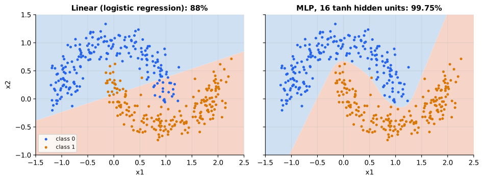
Reading it: both panels show the same two interleaving half-moons, coloured by class; the shaded background is what each model predicts at every point. On the left, a single linear layer can only split the plane with a straight line, so the tips of both moons land on the wrong side (about 88% accuracy). On the right, one hidden tanh layer bends the boundary to follow the gap between the moons (99.75%, one point of 400 wrong). Same data, same optimizer: the only difference is a nonlinearity between two layers.
In code: make_moons builds the two interleaving half-moons (and make_xor the four-point XOR puzzle); train_logistic_regression fits the straight-line baseline in the left panel.
Why it matters: "depth" is only worth anything because of the
activations between layers. linear_stack_collapses shows five stacked
linear layers matching their single-matrix product to 1e-16.
Activation functions: the rule after the sum
Think of different kinds of switch. ReLU is a one-way valve: water flows freely forward, not at all backward. Sigmoid is a dimmer that squeezes any input into 0–1 but barely moves at the extremes. Tanh is the same dimmer centred on zero. GELU is a valve that leaks a little when nearly closed.
Worked example, values you can check on a calculator (the ′ mark, as in sigmoid′, means "the slope of"):
| z | ReLU | sigmoid | sigmoid' | tanh' | GELU |
|---|---|---|---|---|---|
| −1 | 0 | 0.269 | 0.197 | 0.420 | −0.159 |
| 0 | 0 | 0.5 | 0.25 (its maximum) | 1 (its maximum) | 0 |
| 1 | 1 | 0.731 | 0.197 | 0.420 | 0.841 |
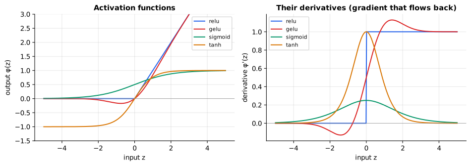
Reading it: the left panel shows each activation's output, the right its derivative, which is how much gradient passes back through it. Look at the tails of the right panel first: sigmoid and tanh derivatives fall to almost zero once |z| passes 3, so a saturated neuron barely learns. Sigmoid's derivative never exceeds 0.25 even at its peak; stack ten such layers and the gradient can shrink by 0.25¹⁰ ≈ 1e-6. ReLU's derivative is a step: exactly 1 for positive inputs (no shrinking) and exactly 0 for negatives. GELU's is a smooth version of that step.
| Function | Formula | Range | Where it's used |
|---|---|---|---|
| ReLU | max(0, z) | [0, ∞) | Hidden layers of CNNs and MLPs. Fast. A neuron stuck negative gets zero gradient forever ("dying ReLU"). |
| GELU | z·Φ(z), Φ = normal CDF | ≈[−0.17, ∞) | Transformers (BERT, GPT-2 and most since). |
| Sigmoid | 1 / (1 + e^−z) | (0, 1) | Binary outputs, and the gates inside LSTMs. |
| Tanh | (e^z − e^−z)/(e^z + e^−z) | (−1, 1) | RNN hidden states; zero-centred. |
| Softmax | e^{z_i} / Σ e^{z_j} | probabilities | The output layer over classes or tokens, and inside attention. |
Reading the formulas: e is Euler's number, about 2.718, and e^z means
"2.718 raised to the power z", which is always positive and grows fast.
Φ(z) is the fraction of a bell curve (the standard normal distribution) that
lies below z: Φ(0) = 0.5, Φ(1) = 0.841. Softmax turns a list of scores
into shares that are all positive and add up to 1: raise e to each score,
then divide each by the total (Σ means "add them all up"). See
primer.notation for each symbol, and primer.ml.attention for softmax
worked through by hand.
In code: relu, sigmoid, tanh and gelu compute each rule, and relu_grad, sigmoid_grad, tanh_grad and gelu_grad compute its slope; gelu_tanh is the cheaper approximation GPT-2 uses, and softmax subtracts the largest score first so nothing overflows.
Why it matters: activation choice decides whether gradients survive a
deep stack. Sigmoid everywhere is why deep networks were hard to train
before 2010; ReLU and residual connections are why they aren't now (see
primer.ml.deep_nets).
Backprop through two layers
Now the assembly line has two stations. The blame from the end first reaches the output weights, then travels back through the hidden layer to the first weights. On the way it passes through the hidden activation, which can shrink it, just as a station that barely changed the product can take only a little of the blame.
Worked example, one input, one hidden unit, one output: x = 1, w1 = 0.5, tanh, w2 = 2, sigmoid, target 1.
| step | value |
|---|---|
| z1 = x·w1 | 0.5 |
| h = tanh(0.5) | 0.4621 |
| z2 = h·w2 | 0.9242 |
| ŷ = σ(0.9242) | 0.7159 |
| dL/dz2 = ŷ − y | −0.2841 |
| dL/dw2 = h · dL/dz2 | −0.1313 |
| dL/dh = dL/dz2 · w2 | −0.5682 |
| dL/dz1 = dL/dh · (1 − h²) | −0.5682 × 0.7864 = −0.4469 |
| dL/dw1 = x · dL/dz1 | −0.4469 |
flowchart LR
  subgraph Forward
    X[X] --> Z1["z1 = X·W1 + b1"] --> H["h = tanh z1"] --> Z2["z2 = h·W2 + b2"] --> P["ŷ = σ z2"] --> L["L = BCE ŷ, y"]
  end
  L -. "ŷ − y" .-> dZ2[dL/dz2]
  dZ2 -. "hᵀ · dz2" .-> dW2[dL/dW2]
  dZ2 -. "dz2 · W2ᵀ" .-> dH[dL/dh]
  dH -. "⊙ 1 − h²" .-> dZ1[dL/dz1]
  dZ1 -. "Xᵀ · dz1" .-> dW1[dL/dW1]
  H -. cached .-> dW2
  H -. cached .-> dZ1
  X -. cached .-> dW1
Reading it: the top row is the forward pass, left to right; the dotted
arrows are the backward pass, starting at the loss and walking back one box
at a time. Each label is one line of MLP.backward, and the worked table
above is that same path with numbers. Notice the three "cached" arrows: the
backward pass reuses h and X from the forward pass. That dependency is why
training must keep every layer's activations in memory, and inference does
not.
For a batch, with binary cross-entropy (the loss for yes/no predictions,
$-[y\ln\hat{y} + (1-y)\ln(1-\hat{y})]$; see primer.ml.losses), which
fuses with sigmoid into the simple error ŷ − y:
Level 3: the formula and its symbols
$$ \frac{\partial L}{\partial z_2} = \hat{y} - y,\; \frac{\partial L}{\partial W_2} = h^\top \frac{\partial L}{\partial z_2},\; \frac{\partial L}{\partial h} = \frac{\partial L}{\partial z_2} W_2^\top,\; \frac{\partial L}{\partial z_1} = \frac{\partial L}{\partial h} \odot (1 - h^2),\; \frac{\partial L}{\partial W_1} = X^\top \frac{\partial L}{\partial z_1} $$
Symbols
| Symbol | Meaning here | In the example (one example, one unit) |
|---|---|---|
| $X$ | inputs, one row per example | $x = 1$ |
| $W_1, W_2$ | first and second layer weights | 0.5, 2 |
| $z_1, z_2$ | each layer's weighted sum, before its activation | 0.5, 0.9242 |
| $h$ | hidden activations, $\tanh(z_1)$ | 0.4621 |
| $\hat{y}$ | "y-hat", the prediction $\sigma(z_2)$ | 0.7159 |
| $y$ | the target | 1 |
| $\sigma$ | sigmoid, squashes any number into 0 to 1 | $\sigma(0.9242) = 0.7159$ |
| $\tanh$ | hyperbolic tangent, squashes into −1 to 1 | $\tanh(0.5) = 0.4621$ |
| $^\top$ | "transpose": flip a matrix so rows become columns, so the shapes line up for the multiply | a scalar is its own transpose |
| $\odot$ | multiply element by element (not a matrix multiply) | $-0.5682 \times 0.7864$ |
| $1 - h^2$ | the slope of tanh at $z_1$ | 0.7864 |
In words: "the error at the output is prediction minus target; each layer's weight gradient is that layer's input times the error arriving at it; to send the error one layer further back, multiply by the weights it came through and by the activation's slope."
With the numbers: $\partial L/\partial z_2 = 0.7159 - 1 = -0.2841$; $\partial L/\partial W_2 = 0.4621 \times -0.2841 = -0.1313$; $\partial L/\partial h = -0.2841 \times 2 = -0.5682$; $\partial L/\partial z_1 = -0.5682 \times 0.7864 = -0.4469$; $\partial L/\partial W_1 = 1 \times -0.4469 = -0.4469$.
Level 3: in Python
In Python:
import math
X, W_1, W_2, y = 1, 0.5, 2, 1
z_1 = X * W_1
h = math.tanh(z_1)
z_2 = h * W_2
# σ(z_2)
y_hat = 1 / (1 + math.exp(-z_2))
# ŷ - y
dL_dz2 = y_hat - y
# hᵀ ∂L/∂z_2
dL_dW2 = h * dL_dz2
# ∂L/∂z_2 W_2ᵀ
dL_dh = dL_dz2 * W_2
# ⊙ (1 - h²), tanh's slope
dL_dz1 = dL_dh * (1 - h ** 2)
# Xᵀ ∂L/∂z_1
dL_dW1 = X * dL_dz1
[round(v, 4) for v in (dL_dz2, dL_dW2, dL_dh, dL_dz1, dL_dW1)]  # → [-0.2841, -0.1313, -0.5682, -0.4469, -0.4469]
The hand-written gradients are checked two ways: a numerical gradient
check (nudge each weight by ±ε and measure the loss change; see
gradient_check) and, in the tests, PyTorch autograd.
In code: tiny_two_layer_example computes every row of the worked table; MLP holds both layers' weights and biases, MLP.loss scores a batch with binary_cross_entropy, and numerical_gradient is the slow nudge-every-weight answer that gradient_check compares against.
Why it matters: the factor (1 − h²) is where gradients shrink. Chain fifty of them and the first layers hear almost nothing: the vanishing gradient problem. The cached activations are why training a model needs several times the memory of serving it.
Batch, step, epoch
Imagine studying a deck of 400 flashcards. You work through a pile of 32, then pause to update your notes; that pause is a step. The pile is a batch. Going through the whole deck once is an epoch; then you shuffle and start again.
Worked example: 400 examples in batches of 32 is 12 full batches plus one of 16, so ⌈400/32⌉ = 13 steps per epoch. Two epochs: 26 steps.
flowchart LR
  E[Epoch: one pass over all 400 examples] --> SH[Shuffle]
  SH --> B1[Batch 1<br/>32 examples] --> S1[Step 1<br/>update weights]
  S1 --> B2[Batch 2] --> S2[Step 2]
  S2 --> D[...] --> B13[Batch 13<br/>last 16 examples] --> S13[Step 13]
  S13 -->|next epoch| E
Reading it: an epoch reshuffles the data and slices it into batches; every batch produces exactly one weight update. Shuffling each epoch means batches differ every time, so the gradient noise doesn't repeat.
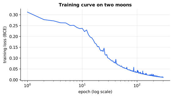
Reading it: the horizontal axis counts epochs on a log scale; the vertical axis is the loss on the whole training set after each one. Loss drops slowly at first while the weights are near their random start, falls steeply once the hidden units find useful features, then flattens as the remaining errors get harder. Plotting this curve is the first thing to do when training anything.
Level 3: the formula and its symbols
$$ \text{steps per epoch} = \left\lceil \frac{N}{B} \right\rceil, \qquad \text{total steps} = \text{epochs} \times \left\lceil \frac{N}{B} \right\rceil $$
Symbols
| Symbol | Meaning here | In the example |
|---|---|---|
| $N$ | number of training examples | 400 |
| $B$ | batch size | 32 |
| $\lceil \cdot \rceil$ | "ceiling": round up to the next whole number (the last, smaller batch still counts as a step) | $\lceil 12.5 \rceil = 13$ |
In words: "an epoch takes as many steps as it takes batches of size B to cover N examples, rounding up."
With the numbers: $\lceil 400 / 32 \rceil = \lceil 12.5 \rceil = 13$ steps per epoch; 2 epochs = 26 steps.
Level 3: in Python
In Python:
import math
N, B, epochs = 400, 32, 2
N / B  # → 12.5
# ⌈N / B⌉: the last, smaller batch still counts
math.ceil(N / B)  # → 13
epochs * math.ceil(N / B)  # → 26
In code: train reshuffles the data every epoch, takes one plain gradient step per batch and records the loss after each epoch; MLP.accuracy reports the fraction of examples classified correctly.
Why it matters: larger batches give smoother gradient estimates and keep GPUs busy, but need more memory. Pretraining a language model runs roughly one epoch over trillions of tokens (it rarely sees the same text twice); fine-tuning runs several epochs over a small dataset, which is why fine-tunes can overfit.
In 20 seconds
- A neuron is a weighted sum plus bias through a nonlinearity; a layer is a matrix multiply; a network is stacked layers.
- Without nonlinearity, depth is pointless: stacked linear layers equal one.
- Training loop: forward, loss, backprop (the chain rule gives a gradient per weight), optimizer step. Repeat.
- Backprop reuses forward activations, so training needs far more memory than inference.
Self-test questions
Why can't you just stack linear layers? Their composition is a single linear map (W1·W2 is just another matrix), so extra layers add parameters but no expressive power.
What does backprop actually compute? The gradient: for every weight, how much a tiny change would change the loss. It applies the chain rule from the output backward, reusing values cached in the forward pass.
Why is ReLU preferred over sigmoid in hidden layers? Sigmoid's derivative is at most 0.25 and near 0 when saturated, so gradients shrink multiplicatively with depth. ReLU's derivative is exactly 1 for positive inputs. The cost: neurons whose input stays negative get zero gradient and "die".
Why does training need more memory than inference? The backward pass needs every layer's activations from the forward pass, so they must be kept until the gradients are computed. Inference can discard each activation as soon as the next layer has used it.
What's the gradient of sigmoid + binary cross-entropy with respect to the logit? ŷ − y: prediction minus target. Clean, bounded and cheap, which is why the two are always fused.
Batch vs. step vs. epoch? A batch is the examples per update, a step is one update, an epoch is one full pass over the data.
The papers behind this lesson
- Rumelhart, Hinton & Williams, Learning representations by back-propagating errors (Nature, 1986): https://www.nature.com/articles/323533a0 Showed that the chain rule, run backwards through a multi-layer network, trains hidden units to discover useful internal features.
- Hendrycks & Gimpel, Gaussian Error Linear Units (GELUs) (2016): https://arxiv.org/abs/1606.08415 Introduced GELU, the smooth ReLU that became the default activation in transformers.
Further reading
- CS231n notes, Backpropagation, intuitions: https://cs231n.github.io/optimization-2/
- CS231n notes, Neural Networks Part 1: https://cs231n.github.io/neural-networks-1/
- Andrej Karpathy, micrograd (autograd in about 100 lines): https://github.com/karpathy/micrograd
- Andrej Karpathy, The spelled-out intro to neural networks and backpropagation: https://www.youtube.com/watch?v=VMj-3S1tku0
- 3Blue1Brown, Neural networks series: https://www.3blue1brown.com/topics/neural-networks
- Michael Nielsen, Neural Networks and Deep Learning, ch. 2: http://neuralnetworksanddeeplearning.com/chap2.html
- Hendrycks & Gimpel, GELU (2016): https://arxiv.org/abs/1606.08415
- PyTorch autograd tutorial: https://pytorch.org/tutorials/beginner/blitz/autograd_tutorial.html
1r""" 2# Neural networks: neurons, activations and backprop by hand 3 4Run: `python -m primer.ml.neural_net` 5 6New to the notation (slopes, Σ, matrices)? `primer.notation` builds every 7symbol used here from zero. This lesson builds on the pipeline picture in 8`primer.ml.big_picture`. 9 10## Level 1: The practitioner's guide 11 12**In one sentence.** A neural network is stacked layers of weighted sums 13with a nonlinear rule after each, and training is one loop, forward pass, 14loss, backpropagation, optimizer step, that nudges every weight in the 15direction that makes the loss smaller. 16 17**When you need it.** You need this the first time you run or read a 18training job rather than call a finished model: a fine-tuning API asks you 19for epochs and a batch size, a training script runs out of memory that 20inference never needed, a loss curve refuses to move, or a custom layer 21needs a gradient you must trust. The tell: a setting in a training config 22(`num_train_epochs`, `per_device_train_batch_size`, `hidden_act`) that you 23copied from an example without knowing which box of the loop it touches. 24You don't need it to prompt a hosted model, and you don't need it to pick 25one from a leaderboard; the forward pass is the only part that runs at 26inference and a vendor has already tuned it. One number from this lesson 27says why depth is worth anything: on the two-moons data, a single linear 28layer scores 88% because it can only draw a straight line, and one hidden 29layer with a nonlinearity scores 99.75% (one point of 400 wrong). 30 31**Your options.** How much of the training loop you own, from the least to 32the most: 33 34| Option | What it does | What it guarantees | What it costs | Where it lives | 35|---|---|---|---|---| 36| Call a trained model | Runs the forward pass only | No gradients, no activations kept: inference memory, and nothing you can break | Per-token pricing, and a model whose weights you cannot move | The API or the model server | 37| Hosted fine-tuning | The vendor runs forward, loss, backward and step on your examples; you set epochs and batch size | No training infrastructure; the loop's four boxes are the vendor's problem | Curated examples, a job that takes hours, a higher per-token price at some vendors | The vendor's fine-tuning API | 38| Framework autograd on your own hardware | `loss.backward()` in PyTorch or `jax.grad` records the forward pass and replays the chain rule backwards over every weight | The gradient is right, for any layer you compose from the framework's pieces | GPU memory several times the inference footprint, because every layer's activations are cached for the backward pass; the loop is yours to debug | Your training script | 39| Backprop by hand, checked numerically | You write the backward pass of a custom layer and compare it with nudging each weight by ±ε | A gradient you can prove: this lesson's check agrees to a relative error of 4.5 × 10⁻⁹ | Time, and a test per layer | A custom layer's backward method | 40 41**How to choose.** Start from what you are changing. 42 43- Behaviour that prompting cannot fix, on a model you cannot host: hosted 44 fine-tuning. Keep the epochs low; fine-tuning runs several passes over a 45 small dataset, and that is how it overfits. 46- A model you host and a dataset of your own: the framework, with the 47 activation the model was built with. Read it from the config 48 (`hidden_act` in a Hugging Face Llama config is `silu`; GPT-2 uses GELU; 49 the transformer paper's feed-forward uses ReLU) and leave it alone, 50 because the trained weights assume it. 51- A new layer, a new loss, a new attention variant: write its backward pass 52 and gradient-check it before training anything on it. A wrong gradient 53 trains quietly and badly. 54- A training run that misbehaves: the fault is in one of the four boxes 55 (data, forward, loss, backward-and-step). Plot the loss per epoch first; 56 its shape (slow start, steep fall, flat tail) is the first diagnostic in 57 this lesson. 58- Whatever you pick, hold out an evaluation set. The loss you train on is 59 the loss the loop minimises, not the score you care about. 60 61**What it costs.** Memory first: the backward pass reuses every layer's 62activations from the forward pass, so training keeps what inference throws 63away and needs several times the memory (this lesson's two-layer trace 64shows the three cached values it depends on). Compute is one matrix 65multiply per layer per direction, and in a transformer most parameters sit 66in the feed-forward layers, which are exactly the two-layer network built 67here. Steps are counted in batches: 400 examples in batches of 32 is 13 68steps per epoch, and two epochs is 26 updates; Hugging Face's 69`TrainingArguments` defaults to 3 epochs, a batch of 8 per device and a 70learning rate of 5 × 10⁻⁵. Pretraining a language model is roughly one 71epoch over trillions of tokens; fine-tuning is several epochs over a small 72set. Quality is paid for in gradient signal: a sigmoid's slope is at most 730.25, so ten sigmoid layers can shrink the gradient by 0.25¹⁰ ≈ 10⁻⁶ before 74it reaches the first weights, while ReLU passes exactly 1 for positive 75inputs. 76 77**What breaks.** 78 79- **The loss doesn't move.** The learning rate is too small (the one-knob 80 example halves the error every step at 0.25 and would crawl at 0.001), or 81 the gradient is dying on the way back: saturated sigmoids pass 0.02 of the 82 signal at |z| = 4, and a ReLU whose input stays negative passes nothing, 83 forever. 84- **The loss explodes or turns NaN.** The step is too big; `primer.ml.optimizers` 85 is the fix. 86- **Out of memory in training, fine in inference.** Cached activations. 87 Halve the batch size before anything else. 88- **Great training loss, poor real results.** Several epochs over a small 89 dataset memorised it; measure on held-out data and stop earlier. 90- **A custom gradient that is wrong.** The network still trains, just not 91 towards anything. Nudge each weight by ±ε and compare: anything below 92 about 10⁻⁶ relative error is right, this lesson's check reports 4.5 × 10⁻⁹. 93- **Depth without nonlinearity.** Five stacked linear layers equal one 94 matrix to 2.2 × 10⁻¹⁶; more parameters, no more power. Every layer needs 95 its activation. 96 97**In the wild.** PyTorch's autograd does this lesson's backward pass for 98billions of weights when you call `loss.backward()`; JAX does it as a 99function transformation, `jax.grad` and `jax.value_and_grad`. PyTorch's 100`nn.Linear` initialises its weights from a uniform range set by the 101fan-in, the rule `primer.ml.deep_nets` explains. Activations in the field: 102GELU in BERT and GPT-2 (Hendrycks and Gimpel, 2016), SwiGLU in Llama 2 103(its paper), and `hidden_act` is the field a Hugging Face config uses to 104name it. Hugging Face's `Trainer` runs the four-box loop with the defaults 105above, and any hosted fine-tuning API runs the same loop behind a form that 106asks for epochs and a batch size. The idea is Rumelhart, Hinton and 107Williams (1986); Karpathy's micrograd is the whole of autograd in about a 108hundred lines. The papers are linked at the end of the lesson. 109 110**Go deeper.** Level 2 trains one knob by hand, builds a neuron and a 111layer, passes blame backwards through the chain rule with every number 112shown, proves why stacked linear layers collapse, compares the activations 113and their slopes, and runs backprop through two layers against a numerical 114check. If you only needed to read a training config, you are done. 115 116## Level 2: How it works, from scratch 117 118A neuron is six lines of arithmetic, a layer is a matrix multiply, and 119training is a loop of four boxes. This level builds each one with numbers 120small enough to check by hand, then verifies the hand-written gradients 121against a numerical check. 122 123## The idea: learning is adjusting knobs to be less wrong 124 125Picture learning to throw darts blindfolded, with a friend calling out "a bit 126high, a bit left". You throw, hear how far off you were, and adjust your arm 127a little. After enough throws your arm "knows" where the bullseye is. A 128neural network learns the same way. Its "arm" is millions of numbers called 129**weights**, and the friend is a formula (the **loss**) that says how far 130off each guess was and which way to adjust. 131 132Two words carry this whole lesson. The **derivative** (or **slope**) of the 133loss with respect to a weight answers "if I nudge this weight up a tiny bit, 134does the loss go up or down, and how fast?" The **gradient** is simply the 135list of those slopes, one per weight. Stepping *against* the gradient is 136walking downhill. (New to the notation? `primer.notation` builds every symbol 137used here from zero.) 138 139Worked example with a single knob: a model with one weight *w* predicts 140y = w·x and should learn y = 3x from the example x = 1, y = 3. The loss is 141(w·1 − 3)². Its slope with respect to w is 2(w − 3). Start at w = 0 and step 142against the slope with step size 0.25: 143 144| step | w | slope 2(w − 3) | new w = w − 0.25·slope | 145|---|---|---|---| 146| 0 | 0 | −6 | 1.5 | 147| 1 | 1.5 | −3 | 2.25 | 148| 2 | 2.25 | −1.5 | 2.625 | 149 150Each step halves the distance to 3. That's all training is. 151 152```mermaid 153flowchart LR 154 D[Batch of examples] --> F[Forward pass<br/>make predictions] 155 F --> L[Loss<br/>how wrong were we?] 156 L --> B[Backpropagation<br/>gradient per weight] 157 B --> O[Optimizer step<br/>adjust weights] 158 O -->|next batch| D 159``` 160 161**Reading it:** follow the arrows clockwise. A batch of examples goes in; the 162forward pass turns them into predictions; the loss scores how wrong those 163predictions were as a single number; backpropagation works out, for every 164weight, which direction would have made that number smaller; the optimizer 165nudges each weight a small step that way. Then the next batch arrives. The 166single-knob table above is one trip around this loop, three times. 167 168The update rule, for every weight at once, with learning rate η: 169 170$$ 171w \leftarrow w - \eta \, \frac{\partial \mathcal{L}}{\partial w} 172$$ 173 174**Symbols** 175 176| Symbol | Meaning here | In the example | 177|---|---|---| 178| $w$ | one weight (a knob the model can turn) | 0 at the start | 179| $\leftarrow$ | "replace the old value with" (an update, not an equation) | | 180| $\eta$ | "eta", the learning rate: how big a step to take | 0.25 | 181| $\mathcal{L}$ | the loss: one number saying how wrong the model is | $(0 - 3)^2 = 9$ | 182| $\partial \mathcal{L} / \partial w$ | the slope of the loss with respect to $w$ (the "partial derivative": how the loss changes when only $w$ moves) | $2(0 - 3) = -6$ | 183 184**In words:** "the new weight is the old weight minus the learning rate times 185the slope of the loss at the old weight." 186 187**With the numbers:** $w \leftarrow 0 - 0.25 \times (-6) = 1.5$, the first row 188of the table. 189 190**In Python:** 191 192```python 193w, eta, target = 0.0, 0.25, 3.0 194for step in range(3): 195 # ∂L/∂w for the loss (w - 3)² 196 slope = 2 * (w - target) 197 # w ← w - η ∂L/∂w 198 w = w - eta * slope 199 print(w) # → 1.5 2.25 2.625 200``` 201 202`learn_one_weight` runs the table above; `train` runs the loop for a real 203network. 204 205**Why it matters:** this loop is identical for a spam filter and for a 206frontier language model. Only the size of the network, the data, and the 207loss change. When a training run misbehaves, the fault is in one of these 208four boxes. 209 210## A neuron: a weighted vote followed by a decision 211 212Think of a judge at a cooking contest. They score taste, presentation and 213originality, but care about taste most, so they weight it more. They add a 214baseline ("everyone starts at half a point"), then apply a rule to turn the 215total into a verdict ("negative totals count as zero"). That is a neuron: 216**weights** are how much each input matters, the **bias** is the baseline, 217and the **activation function** is the rule. 218 219Worked example: inputs (2, 3), weights (0.5, 1.0), bias 0.5. 220Weighted sum: 2 × 0.5 + 3 × 1.0 + 0.5 = 4.5. The ReLU rule keeps positive 221values, so the output is 4.5. 222 223```mermaid 224flowchart LR 225 X1((x1 = 2)) -- "× w1 = 0.5" --> S["Sum + bias<br/>1.0 + 3.0 + 0.5 = 4.5"] 226 X2((x2 = 3)) -- "× w2 = 1.0" --> S 227 B((bias 0.5)) --> S 228 S --> A["Activation φ<br/>ReLU(4.5) = 4.5"] 229 A --> Y((y = 4.5)) 230``` 231 232**Reading it:** each input travels along an edge that multiplies it by that 233edge's weight; the middle node adds the products and the bias; the 234activation reshapes the sum into the output. A **layer** is this picture 235repeated side by side, every input wired to every neuron, which is exactly a 236matrix multiply. A **network** is layers stacked. 237 238$$ 239y = \phi\left(\sum_i w_i x_i + b\right) = \phi(w \cdot x + b), \qquad 240\text{a layer: } Y = \phi(XW + b) 241$$ 242 243**Symbols** 244 245| Symbol | Meaning here | In the example | 246|---|---|---| 247| $x_i$ | the $i$-th input | $x_1 = 2$, $x_2 = 3$ | 248| $w_i$ | the weight on the $i$-th input | $w_1 = 0.5$, $w_2 = 1.0$ | 249| $i$ | a counter over the inputs | 1, 2 | 250| $\sum_i$ | "add up the following for every $i$" | $w_1x_1 + w_2x_2$ | 251| $b$ | the bias (the baseline added to every sum) | 0.5 | 252| $w \cdot x$ | the **dot product**: multiply matching entries of two lists, then add | $0.5·2 + 1.0·3 = 4.0$ | 253| $\phi$ | "phi", the activation function | ReLU | 254| $y$ | the neuron's output | 4.5 | 255| $X$ | a batch of inputs, one example per row | shape (batch, inputs) | 256| $W$ | a layer's weights, one column per neuron | shape (inputs, neurons) | 257| $XW$ | **matrix multiply**: every row of $X$ dotted with every column of $W$ | shape (batch, neurons) | 258| $Y$ | every neuron's output for every example | shape (batch, neurons) | 259 260**In words:** "multiply each input by its weight, add them up, add the 261bias, and pass the total through the activation function." 262 263**With the numbers:** $y = \text{ReLU}(0.5 \cdot 2 + 1.0 \cdot 3 + 0.5) = 264\text{ReLU}(4.5) = 4.5$. 265 266**In Python:** 267 268```python 269x = [2, 3] 270w = [0.5, 1.0] 271b = 0.5 272# ReLU: keep positives, zero the rest 273def phi(z): return max(0.0, z) 274# w · x = Σ_i w_i x_i 275sum(w_i * x_i for w_i, x_i in zip(w, x)) # → 4.0 276# y = φ(w · x + b) 277phi(sum(w_i * x_i for w_i, x_i in zip(w, x)) + b) # → 4.5 278``` 279 280**Why it matters:** every dense layer in every model is this, including the 281feed-forward half of each transformer block, where most of a language 282model's parameters live. `MLP.forward` is two of these layers in six lines. 283 284## Backpropagation: passing the blame backwards 285 286Picture an assembly line that produced a faulty product. The inspector at the 287end measures how bad it is and passes the complaint back. Each station 288works out how much of the fault was its own doing, based on what it received 289and what it did to it, and passes the rest further back. Every station ends 290up knowing exactly how to adjust its own machine. Backpropagation is that 291blame-passing, done with derivatives. 292 293Worked example, continuing the neuron: the target was 5, so the loss is 294(5 − 4.5)² = 0.25. 295 296| link | local derivative | running blame | 297|---|---|---| 298| loss → y | 2(y − 5) = −1 | −1 | 299| y → z (ReLU, z > 0) | 1 | −1 | 300| z → w1 | x1 = 2 | **−2** | 301| z → w2 | x2 = 3 | **−3** | 302| z → b | 1 | **−1** | 303 304One step with learning rate 0.01 moves weights to (0.52, 1.03) and bias to 3050.51. The new output is 4.64 and the loss drops from 0.25 to 0.1296. The 306weight whose input was bigger (3) received the bigger share of blame and 307moved more. 308 309```mermaid 310flowchart RL 311 L["Loss (5 − y)² = 0.25"] -- "dL/dy = −1" --> Y[y = ReLU z] 312 Y -- "dy/dz = 1" --> Z[z = w·x + b] 313 Z -- "× x1 = 2 → dL/dw1 = −2" --> W1[w1] 314 Z -- "× x2 = 3 → dL/dw2 = −3" --> W2[w2] 315 Z -- "× 1 → dL/db = −1" --> Bb[b] 316``` 317 318**Reading it:** this is the neuron read right to left. Start at the loss and 319multiply the local derivatives along each path; that product is the chain 320rule. All paths share the first two links (−1 × 1), then split. Each weight's 321gradient is the blame arriving at the sum times the input that weight 322multiplied. Negative gradient means "increase me to reduce the loss". 323 324$$ 325\frac{\partial \mathcal{L}}{\partial w_i} = 326\frac{\partial \mathcal{L}}{\partial y}\cdot\frac{\partial y}{\partial z}\cdot\frac{\partial z}{\partial w_i} 327= 2(y - t)\cdot\phi'(z)\cdot x_i 328$$ 329 330This is the **chain rule**: when a change passes through several steps, the 331overall rate of change is the product of each step's rate of change. If 332turning a knob moves a gear 3× as fast, and that gear moves a needle 2× as 333fast, the knob moves the needle 6× as fast. 334 335**Symbols** 336 337| Symbol | Meaning here | In the example | 338|---|---|---| 339| $\mathcal{L}$ | the loss $(t - y)^2$ | 0.25 | 340| $t$ | the target (the right answer) | 5 | 341| $y$ | the neuron's output | 4.5 | 342| $z$ | the weighted sum before the activation | 4.5 | 343| $\partial \mathcal{L}/\partial y$ | how the loss changes as the output changes | $2(4.5 - 5) = -1$ | 344| $\partial y/\partial z$ | how the output changes as the sum changes: the activation's slope $\phi'(z)$ | ReLU slope at 4.5 = 1 | 345| $\partial z/\partial w_i$ | how the sum changes as weight $i$ changes: just its input $x_i$ | $x_2 = 3$ | 346| $\phi'$ | the activation's derivative (slope) | 1 for ReLU when $z > 0$ | 347 348**In words:** "the blame on a weight is how much the loss cares about the 349output, times how much the output cares about the sum, times how much the 350sum cares about that weight." 351 352**With the numbers:** for $w_2$: $(-1) \times 1 \times 3 = -3$; for $w_1$: 353$(-1) \times 1 \times 2 = -2$. 354 355**In Python:** 356 357```python 358x, t, z = [2, 3], 5, 4.5 359# ReLU(4.5) 360y = max(0.0, z) 361# ∂L/∂y 362dL_dy = 2 * (y - t) 363# φ'(z): ReLU's slope 364dy_dz = 1 if z > 0 else 0 365# × ∂z/∂w_i = x_i, for w_1 and w_2 366[dL_dy * dy_dz * x_i for x_i in x] # → [-2.0, -3.0] 367# one step, learning rate 0.01 368w = [0.5 - 0.01 * -2.0, 1.0 - 0.01 * -3.0] 369b = 0.5 - 0.01 * -1.0 370y_new = w[0] * x[0] + w[1] * x[1] + b 371# the new output and the smaller loss 372round(y_new, 2), round((t - y_new) ** 2, 4) # → (4.64, 0.1296) 373``` 374 375`one_neuron_worked_example` computes every row of the table. 376 377**Why it matters:** PyTorch's `loss.backward()` does exactly this, for 378billions of weights, by recording the forward computation and replaying it 379backwards. Knowing it is just the chain rule is what lets you reason about 380vanishing gradients, memory use, and why some architectures train and others 381don't. 382 383## Why the nonlinearity is essential 384 385Stack three sheets of tinted glass and you get one darker sheet of glass: no 386arrangement of flat panes can bend light around a corner. Linear layers are 387flat panes. However many you stack, the result is one linear layer, which can 388only separate classes with a straight line. The activation function is the 389bend. 390 391Worked example in one dimension: a layer that multiplies by 3, followed by a 392layer that multiplies by 2, is the same as one layer that multiplies by 6. 393With a ReLU between them, inputs −1 and 1 give 0 and 6. No single 394multiplication does that. 395 396```mermaid 397flowchart LR 398 subgraph NoAct["Without activation"] 399 a1[X] --> a2[·W1] --> a3[·W2] --> a4[·W3] --> a5["= X·(W1W2W3)<br/>one matrix"] 400 end 401 subgraph WithAct["With activation"] 402 b1[X] --> b2[·W1] --> b3[φ] --> b4[·W2] --> b5[φ] --> b6[·W3] --> b7[curved<br/>decision boundary] 403 end 404``` 405 406**Reading it:** in the top row the multiplications are chained with nothing 407in between, and associativity lets you multiply the weights together first: 408three layers equal one. In the bottom row a nonlinearity φ sits between the 409multiplies, the product can no longer be pre-computed, and the network can 410bend its decision boundary. 411 412$$ 413(XW_1)W_2 = X(W_1W_2) \quad\text{but}\quad \phi(XW_1)W_2 \neq X W' \text{ for any } W' 414$$ 415 416**Symbols** 417 418| Symbol | Meaning here | In the example | 419|---|---|---| 420| $X$ | the inputs | $x = -1$ or $x = 1$ | 421| $W_1, W_2$ | two layers' weights | 3 and 2 | 422| $W_1W_2$ | the two layers multiplied into one | 6 | 423| $\phi$ | an activation between the layers | ReLU | 424| $W'$ | any single weight you might try instead | none works | 425| $\neq$ | "is not equal to" | | 426 427**In words:** "two linear layers in a row are the same as one linear layer, 428but put an activation between them and no single layer can copy them." 429 430**With the numbers:** without ReLU, $-1 \to -3 \to -6$ and $1 \to 3 \to 6$, 431exactly $6x$. With ReLU, $-1 \to -3 \to 0 \to 0$ and $1 \to 3 \to 3 \to 6$. 432A single weight $W'$ would need $-W' = 0$ and $W' = 6$ at once: impossible. 433 434**In Python:** 435 436```python 437W_1, W_2 = 3, 2 438# ReLU 439def phi(z): return max(0, z) 440# (X W_1) W_2 ... 441[(x * W_1) * W_2 for x in [-1, 1]] # → [-6, 6] 442# ... equals X (W_1 W_2): one layer of 6 443[x * (W_1 * W_2) for x in [-1, 1]] # → [-6, 6] 444# φ(X W_1) W_2: no single W' gives 0 and 6 445[phi(x * W_1) * W_2 for x in [-1, 1]] # → [0, 6] 446``` 447 448 449 450**Reading it:** both panels show the same two interleaving half-moons, 451coloured by class; the shaded background is what each model predicts at 452every point. On the left, a single linear layer can only split the plane with 453a straight line, so the tips of both moons land on the wrong side (about 88% 454accuracy). On the right, one hidden tanh layer bends the boundary to follow 455the gap between the moons (99.75%, one point of 400 wrong). Same data, same optimizer: the only 456difference is a nonlinearity between two layers. 457 458**In code:** `make_moons` builds the two interleaving half-moons (and `make_xor` the four-point XOR puzzle); `train_logistic_regression` fits the straight-line baseline in the left panel. 459 460**Why it matters:** "depth" is only worth anything because of the 461activations between layers. `linear_stack_collapses` shows five stacked 462linear layers matching their single-matrix product to 1e-16. 463 464## Activation functions: the rule after the sum 465 466Think of different kinds of switch. **ReLU** is a one-way valve: water flows 467freely forward, not at all backward. **Sigmoid** is a dimmer that squeezes 468any input into 0–1 but barely moves at the extremes. **Tanh** is the same 469dimmer centred on zero. **GELU** is a valve that leaks a little when nearly 470closed. 471 472Worked example, values you can check on a calculator (the ′ mark, as in 473sigmoid′, means "the slope of"): 474 475| z | ReLU | sigmoid | sigmoid' | tanh' | GELU | 476|---|---|---|---|---|---| 477| −1 | 0 | 0.269 | 0.197 | 0.420 | −0.159 | 478| 0 | 0 | 0.5 | **0.25** (its maximum) | **1** (its maximum) | 0 | 479| 1 | 1 | 0.731 | 0.197 | 0.420 | 0.841 | 480 481 482 483**Reading it:** the left panel shows each activation's output, the right its 484derivative, which is how much gradient passes back through it. Look at the 485tails of the right panel first: sigmoid and tanh derivatives fall to almost 486zero once |z| passes 3, so a *saturated* neuron barely learns. Sigmoid's 487derivative never exceeds 0.25 even at its peak; stack ten such layers and the 488gradient can shrink by 0.25¹⁰ ≈ 1e-6. ReLU's derivative is a step: exactly 1 489for positive inputs (no shrinking) and exactly 0 for negatives. GELU's is a 490smooth version of that step. 491 492| Function | Formula | Range | Where it's used | 493|---|---|---|---| 494| ReLU | max(0, z) | [0, ∞) | Hidden layers of CNNs and MLPs. Fast. A neuron stuck negative gets zero gradient forever ("dying ReLU"). | 495| GELU | z·Φ(z), Φ = normal CDF | ≈[−0.17, ∞) | Transformers (BERT, GPT-2 and most since). | 496| Sigmoid | 1 / (1 + e^−z) | (0, 1) | Binary outputs, and the gates inside LSTMs. | 497| Tanh | (e^z − e^−z)/(e^z + e^−z) | (−1, 1) | RNN hidden states; zero-centred. | 498| Softmax | e^{z_i} / Σ e^{z_j} | probabilities | The output layer over classes or tokens, and inside attention. | 499 500Reading the formulas: *e* is Euler's number, about 2.718, and e^z means 501"2.718 raised to the power z", which is always positive and grows fast. 502Φ(z) is the fraction of a bell curve (the standard normal distribution) that 503lies below z: Φ(0) = 0.5, Φ(1) = 0.841. **Softmax** turns a list of scores 504into shares that are all positive and add up to 1: raise *e* to each score, 505then divide each by the total (Σ means "add them all up"). See 506`primer.notation` for each symbol, and `primer.ml.attention` for softmax 507worked through by hand. 508 509**In code:** `relu`, `sigmoid`, `tanh` and `gelu` compute each rule, and `relu_grad`, `sigmoid_grad`, `tanh_grad` and `gelu_grad` compute its slope; `gelu_tanh` is the cheaper approximation GPT-2 uses, and `softmax` subtracts the largest score first so nothing overflows. 510 511**Why it matters:** activation choice decides whether gradients survive a 512deep stack. Sigmoid everywhere is why deep networks were hard to train 513before 2010; ReLU and residual connections are why they aren't now (see 514`primer.ml.deep_nets`). 515 516## Backprop through two layers 517 518Now the assembly line has two stations. The blame from the end first reaches 519the output weights, then travels back through the hidden layer to the first 520weights. On the way it passes through the hidden activation, which can 521shrink it, just as a station that barely changed the product can take only a 522little of the blame. 523 524Worked example, one input, one hidden unit, one output: x = 1, w1 = 0.5, 525tanh, w2 = 2, sigmoid, target 1. 526 527| step | value | 528|---|---| 529| z1 = x·w1 | 0.5 | 530| h = tanh(0.5) | 0.4621 | 531| z2 = h·w2 | 0.9242 | 532| ŷ = σ(0.9242) | 0.7159 | 533| dL/dz2 = ŷ − y | −0.2841 | 534| dL/dw2 = h · dL/dz2 | −0.1313 | 535| dL/dh = dL/dz2 · w2 | −0.5682 | 536| dL/dz1 = dL/dh · (1 − h²) | −0.5682 × 0.7864 = −0.4469 | 537| dL/dw1 = x · dL/dz1 | −0.4469 | 538 539```mermaid 540flowchart LR 541 subgraph Forward 542 X[X] --> Z1["z1 = X·W1 + b1"] --> H["h = tanh z1"] --> Z2["z2 = h·W2 + b2"] --> P["ŷ = σ z2"] --> L["L = BCE ŷ, y"] 543 end 544 L -. "ŷ − y" .-> dZ2[dL/dz2] 545 dZ2 -. "hᵀ · dz2" .-> dW2[dL/dW2] 546 dZ2 -. "dz2 · W2ᵀ" .-> dH[dL/dh] 547 dH -. "⊙ 1 − h²" .-> dZ1[dL/dz1] 548 dZ1 -. "Xᵀ · dz1" .-> dW1[dL/dW1] 549 H -. cached .-> dW2 550 H -. cached .-> dZ1 551 X -. cached .-> dW1 552``` 553 554**Reading it:** the top row is the forward pass, left to right; the dotted 555arrows are the backward pass, starting at the loss and walking back one box 556at a time. Each label is one line of `MLP.backward`, and the worked table 557above is that same path with numbers. Notice the three "cached" arrows: the 558backward pass reuses h and X from the forward pass. That dependency is why 559training must keep every layer's activations in memory, and inference does 560not. 561 562For a batch, with binary cross-entropy (the loss for yes/no predictions, 563$-[y\ln\hat{y} + (1-y)\ln(1-\hat{y})]$; see `primer.ml.losses`), which 564fuses with sigmoid into the simple error ŷ − y: 565 566$$ 567\frac{\partial L}{\partial z_2} = \hat{y} - y,\; 568\frac{\partial L}{\partial W_2} = h^\top \frac{\partial L}{\partial z_2},\; 569\frac{\partial L}{\partial h} = \frac{\partial L}{\partial z_2} W_2^\top,\; 570\frac{\partial L}{\partial z_1} = \frac{\partial L}{\partial h} \odot (1 - h^2),\; 571\frac{\partial L}{\partial W_1} = X^\top \frac{\partial L}{\partial z_1} 572$$ 573 574**Symbols** 575 576| Symbol | Meaning here | In the example (one example, one unit) | 577|---|---|---| 578| $X$ | inputs, one row per example | $x = 1$ | 579| $W_1, W_2$ | first and second layer weights | 0.5, 2 | 580| $z_1, z_2$ | each layer's weighted sum, before its activation | 0.5, 0.9242 | 581| $h$ | hidden activations, $\tanh(z_1)$ | 0.4621 | 582| $\hat{y}$ | "y-hat", the prediction $\sigma(z_2)$ | 0.7159 | 583| $y$ | the target | 1 | 584| $\sigma$ | sigmoid, squashes any number into 0 to 1 | $\sigma(0.9242) = 0.7159$ | 585| $\tanh$ | hyperbolic tangent, squashes into −1 to 1 | $\tanh(0.5) = 0.4621$ | 586| $^\top$ | "transpose": flip a matrix so rows become columns, so the shapes line up for the multiply | a scalar is its own transpose | 587| $\odot$ | multiply element by element (not a matrix multiply) | $-0.5682 \times 0.7864$ | 588| $1 - h^2$ | the slope of tanh at $z_1$ | 0.7864 | 589 590**In words:** "the error at the output is prediction minus target; each 591layer's weight gradient is that layer's input times the error arriving at it; 592to send the error one layer further back, multiply by the weights it came 593through and by the activation's slope." 594 595**With the numbers:** $\partial L/\partial z_2 = 0.7159 - 1 = -0.2841$; 596$\partial L/\partial W_2 = 0.4621 \times -0.2841 = -0.1313$; 597$\partial L/\partial h = -0.2841 \times 2 = -0.5682$; 598$\partial L/\partial z_1 = -0.5682 \times 0.7864 = -0.4469$; 599$\partial L/\partial W_1 = 1 \times -0.4469 = -0.4469$. 600 601**In Python:** 602 603```python 604import math 605X, W_1, W_2, y = 1, 0.5, 2, 1 606z_1 = X * W_1 607h = math.tanh(z_1) 608z_2 = h * W_2 609# σ(z_2) 610y_hat = 1 / (1 + math.exp(-z_2)) 611# ŷ - y 612dL_dz2 = y_hat - y 613# hᵀ ∂L/∂z_2 614dL_dW2 = h * dL_dz2 615# ∂L/∂z_2 W_2ᵀ 616dL_dh = dL_dz2 * W_2 617# ⊙ (1 - h²), tanh's slope 618dL_dz1 = dL_dh * (1 - h ** 2) 619# Xᵀ ∂L/∂z_1 620dL_dW1 = X * dL_dz1 621[round(v, 4) for v in (dL_dz2, dL_dW2, dL_dh, dL_dz1, dL_dW1)] # → [-0.2841, -0.1313, -0.5682, -0.4469, -0.4469] 622``` 623 624The hand-written gradients are checked two ways: a **numerical gradient 625check** (nudge each weight by ±ε and measure the loss change; see 626`gradient_check`) and, in the tests, PyTorch autograd. 627 628**In code:** `tiny_two_layer_example` computes every row of the worked table; `MLP` holds both layers' weights and biases, `MLP.loss` scores a batch with `binary_cross_entropy`, and `numerical_gradient` is the slow nudge-every-weight answer that `gradient_check` compares against. 629 630**Why it matters:** the factor (1 − h²) is where gradients shrink. Chain 631fifty of them and the first layers hear almost nothing: the vanishing 632gradient problem. The cached activations are why training a model needs 633several times the memory of serving it. 634 635## Batch, step, epoch 636 637Imagine studying a deck of 400 flashcards. You work through a pile of 32, 638then pause to update your notes; that pause is a **step**. The pile is a 639**batch**. Going through the whole deck once is an **epoch**; then you 640shuffle and start again. 641 642Worked example: 400 examples in batches of 32 is 12 full batches plus one of 64316, so ⌈400/32⌉ = 13 steps per epoch. Two epochs: 26 steps. 644 645```mermaid 646flowchart LR 647 E[Epoch: one pass over all 400 examples] --> SH[Shuffle] 648 SH --> B1[Batch 1<br/>32 examples] --> S1[Step 1<br/>update weights] 649 S1 --> B2[Batch 2] --> S2[Step 2] 650 S2 --> D[...] --> B13[Batch 13<br/>last 16 examples] --> S13[Step 13] 651 S13 -->|next epoch| E 652``` 653 654**Reading it:** an epoch reshuffles the data and slices it into batches; 655every batch produces exactly one weight update. Shuffling each epoch means 656batches differ every time, so the gradient noise doesn't repeat. 657 658 659 660**Reading it:** the horizontal axis counts epochs on a log scale; the vertical 661axis is the loss on the whole training set after each one. Loss drops slowly 662at first while the weights are near their random start, falls steeply once 663the hidden units find useful features, then flattens as the remaining errors 664get harder. Plotting this curve is the first thing to do when training 665anything. 666 667$$ 668\text{steps per epoch} = \left\lceil \frac{N}{B} \right\rceil, \qquad 669\text{total steps} = \text{epochs} \times \left\lceil \frac{N}{B} \right\rceil 670$$ 671 672**Symbols** 673 674| Symbol | Meaning here | In the example | 675|---|---|---| 676| $N$ | number of training examples | 400 | 677| $B$ | batch size | 32 | 678| $\lceil \cdot \rceil$ | "ceiling": round up to the next whole number (the last, smaller batch still counts as a step) | $\lceil 12.5 \rceil = 13$ | 679 680**In words:** "an epoch takes as many steps as it takes batches of size B to 681cover N examples, rounding up." 682 683**With the numbers:** $\lceil 400 / 32 \rceil = \lceil 12.5 \rceil = 13$ steps 684per epoch; 2 epochs = 26 steps. 685 686**In Python:** 687 688```python 689import math 690N, B, epochs = 400, 32, 2 691N / B # → 12.5 692# ⌈N / B⌉: the last, smaller batch still counts 693math.ceil(N / B) # → 13 694epochs * math.ceil(N / B) # → 26 695``` 696 697**In code:** `train` reshuffles the data every epoch, takes one plain gradient step per batch and records the loss after each epoch; `MLP.accuracy` reports the fraction of examples classified correctly. 698 699**Why it matters:** larger batches give smoother gradient estimates and keep 700GPUs busy, but need more memory. Pretraining a language model runs roughly 701one epoch over trillions of tokens (it rarely sees the same text twice); 702fine-tuning runs several epochs over a small dataset, which is why 703fine-tunes can overfit. 704 705## In 20 seconds 706- A neuron is a weighted sum plus bias through a nonlinearity; a layer is a 707 matrix multiply; a network is stacked layers. 708- Without nonlinearity, depth is pointless: stacked linear layers equal one. 709- Training loop: forward, loss, backprop (the chain rule gives a gradient per 710 weight), optimizer step. Repeat. 711- Backprop reuses forward activations, so training needs far more memory 712 than inference. 713 714## Self-test questions 715 716**Why can't you just stack linear layers?** 717Their composition is a single linear map (W1·W2 is just another matrix), so 718extra layers add parameters but no expressive power. 719 720**What does backprop actually compute?** 721The gradient: for every weight, how much a tiny change would change the loss. 722It applies the chain rule from the output backward, reusing values cached in 723the forward pass. 724 725**Why is ReLU preferred over sigmoid in hidden layers?** 726Sigmoid's derivative is at most 0.25 and near 0 when saturated, so gradients 727shrink multiplicatively with depth. ReLU's derivative is exactly 1 for 728positive inputs. The cost: neurons whose input stays negative get zero 729gradient and "die". 730 731**Why does training need more memory than inference?** 732The backward pass needs every layer's activations from the forward pass, so 733they must be kept until the gradients are computed. Inference can discard 734each activation as soon as the next layer has used it. 735 736**What's the gradient of sigmoid + binary cross-entropy with respect to the logit?** 737ŷ − y: prediction minus target. Clean, bounded and cheap, which is why the 738two are always fused. 739 740**Batch vs. step vs. epoch?** 741A batch is the examples per update, a step is one update, an epoch is one 742full pass over the data. 743 744## The papers behind this lesson 745 746- Rumelhart, Hinton & Williams, *Learning representations by back-propagating errors* (Nature, 1986): https://www.nature.com/articles/323533a0 747 Showed that the chain rule, run backwards through a multi-layer network, trains hidden units to discover useful internal features. 748- Hendrycks & Gimpel, *Gaussian Error Linear Units (GELUs)* (2016): https://arxiv.org/abs/1606.08415 749 Introduced GELU, the smooth ReLU that became the default activation in transformers. 750 751## Further reading 752- CS231n notes, *Backpropagation, intuitions*: https://cs231n.github.io/optimization-2/ 753- CS231n notes, *Neural Networks Part 1*: https://cs231n.github.io/neural-networks-1/ 754- Andrej Karpathy, *micrograd* (autograd in about 100 lines): https://github.com/karpathy/micrograd 755- Andrej Karpathy, *The spelled-out intro to neural networks and backpropagation*: https://www.youtube.com/watch?v=VMj-3S1tku0 756- 3Blue1Brown, *Neural networks* series: https://www.3blue1brown.com/topics/neural-networks 757- Michael Nielsen, *Neural Networks and Deep Learning*, ch. 2: http://neuralnetworksanddeeplearning.com/chap2.html 758- Hendrycks & Gimpel, *GELU* (2016): https://arxiv.org/abs/1606.08415 759- PyTorch autograd tutorial: https://pytorch.org/tutorials/beginner/blitz/autograd_tutorial.html 760""" 761 762from __future__ import annotations 763 764import math 765from dataclasses import dataclass, field 766 767import numpy as np 768 769from primer._show import banner, say, table, takeaway 770 771# --------------------------------------------------------------------------- 772# 0. One knob: the whole training idea with a single weight 773# --------------------------------------------------------------------------- 774 775 776def learn_one_weight(steps: int = 3, lr: float = 0.25) -> list[float]: 777 """Gradient descent on loss (w·1 − 3)², starting from w = 0. Returns w after each step. 778 779 The slope is 2(w − 3); with lr 0.25 each step moves w halfway to 3. 780 """ 781 w, history = 0.0, [0.0] 782 for _ in range(steps): 783 slope = 2 * (w * 1.0 - 3.0) 784 w -= lr * slope 785 history.append(w) 786 return history 787 788 789# --------------------------------------------------------------------------- 790# 1. One neuron, by hand 791# --------------------------------------------------------------------------- 792 793 794def one_neuron_worked_example(lr: float = 0.01) -> dict: 795 """Forward pass, squared-error loss, gradients, and one SGD step for one ReLU neuron. 796 797 Inputs (2, 3), weights (0.5, 1.0), bias 0.5, target 5. 798 """ 799 x = np.array([2.0, 3.0]) 800 w = np.array([0.5, 1.0]) 801 b = 0.5 802 target = 5.0 803 804 # Forward. 805 z = w @ x + b # weighted sum: 2*0.5 + 3*1.0 + 0.5 = 4.5 806 y = relu(z) # positive, so unchanged: 4.5 807 loss = (target - y) ** 2 # 0.25 808 809 # Backward, one chain-rule link at a time. 810 dL_dy = 2 * (y - target) # d/dy (t - y)^2 = -2 (t - y) = -1.0 811 dy_dz = relu_grad(z) # 1 because z > 0 812 dL_dz = dL_dy * dy_dz 813 dL_dw = dL_dz * x # dz/dw_i = x_i, so the weight with the bigger input gets the bigger gradient 814 dL_db = dL_dz # dz/db = 1 815 816 # SGD: step *against* the gradient. 817 w_new = w - lr * dL_dw 818 b_new = b - lr * dL_db 819 y_new = relu(w_new @ x + b_new) 820 return dict( 821 z=float(z), 822 y=float(y), 823 loss=float(loss), 824 dL_dw=dL_dw, 825 dL_db=float(dL_db), 826 w_new=w_new, 827 b_new=float(b_new), 828 y_new=float(y_new), 829 loss_new=float((target - y_new) ** 2), 830 ) 831 832 833# --------------------------------------------------------------------------- 834# 2. Activation functions and their derivatives 835# --------------------------------------------------------------------------- 836 837 838def relu(z): 839 return np.maximum(0.0, z) 840 841 842def relu_grad(z): 843 # The derivative at exactly 0 is undefined; frameworks use 0. It never matters in practice. 844 return (np.asarray(z) > 0).astype(float) 845 846 847def sigmoid(z): 848 # Split by sign so exp never overflows: for z << 0 use e^z / (1 + e^z). 849 z = np.asarray(z, dtype=float) 850 out = np.empty_like(z) 851 pos = z >= 0 852 out[pos] = 1 / (1 + np.exp(-z[pos])) 853 ez = np.exp(z[~pos]) 854 out[~pos] = ez / (1 + ez) 855 return out 856 857 858def sigmoid_grad(z): 859 s = sigmoid(z) 860 return s * (1 - s) # peaks at 0.25 when z = 0 861 862 863def tanh(z): 864 return np.tanh(z) 865 866 867def tanh_grad(z): 868 return 1 - np.tanh(z) ** 2 # peaks at 1 when z = 0 869 870 871_erf = np.vectorize(math.erf) 872 873 874def gelu(z): 875 """Exact GELU: z * Φ(z), where Φ is the standard normal CDF. 876 877 Intuition: scale each input by the probability that a standard normal is 878 below it. Large positives pass through, large negatives go to 0, and 879 small negatives leak a little (unlike ReLU's hard cutoff). 880 """ 881 z = np.asarray(z, dtype=float) 882 return 0.5 * z * (1 + _erf(z / math.sqrt(2))) 883 884 885def gelu_tanh(z): 886 """The tanh approximation used by GPT-2 and many kernels.""" 887 z = np.asarray(z, dtype=float) 888 return 0.5 * z * (1 + np.tanh(math.sqrt(2 / math.pi) * (z + 0.044715 * z**3))) 889 890 891def gelu_grad(z): 892 z = np.asarray(z, dtype=float) 893 cdf = 0.5 * (1 + _erf(z / math.sqrt(2))) 894 pdf = np.exp(-0.5 * z**2) / math.sqrt(2 * math.pi) 895 return cdf + z * pdf 896 897 898def softmax(z, axis: int = -1): 899 """Stable softmax (see primer.ml.attention.softmax for the full story).""" 900 z = np.asarray(z, dtype=float) 901 e = np.exp(z - z.max(axis=axis, keepdims=True)) 902 return e / e.sum(axis=axis, keepdims=True) 903 904 905ACTIVATIONS = { 906 "relu": (relu, relu_grad), 907 "gelu": (gelu, gelu_grad), 908 "sigmoid": (sigmoid, sigmoid_grad), 909 "tanh": (tanh, tanh_grad), 910} 911 912 913def tiny_two_layer_example() -> dict: 914 """Backprop through x → (w1, tanh) → (w2, sigmoid) → BCE with scalars you can check by hand. 915 916 x = 1, w1 = 0.5, w2 = 2, target 1, no biases. 917 """ 918 x, w1, w2, y = 1.0, 0.5, 2.0, 1.0 919 z1 = x * w1 920 h = float(np.tanh(z1)) 921 z2 = h * w2 922 y_hat = float(sigmoid(np.array([z2]))[0]) 923 dL_dz2 = y_hat - y # sigmoid + BCE fuse to prediction − target 924 dL_dw2 = h * dL_dz2 # the output weight's input was h 925 dL_dh = dL_dz2 * w2 # blame sent back through w2 926 dL_dz1 = dL_dh * (1 - h**2) # shrunk by tanh's slope at z1 927 dL_dw1 = x * dL_dz1 928 return dict(z1=z1, h=h, z2=z2, y_hat=y_hat, dL_dz2=dL_dz2, dL_dw2=dL_dw2, dL_dh=dL_dh, dL_dz1=dL_dz1, dL_dw1=dL_dw1) 929 930 931# --------------------------------------------------------------------------- 932# 3. Why nonlinearity matters 933# --------------------------------------------------------------------------- 934 935 936def linear_stack_collapses(n_layers: int = 5, d: int = 4, seed: int = 0) -> float: 937 """Return max |difference| between a deep linear stack and its single-matrix equivalent. 938 939 It's ~1e-15 (floating-point noise): the deep stack *is* one linear layer. 940 """ 941 rng = np.random.default_rng(seed) 942 Ws = [rng.standard_normal((d, d)) / np.sqrt(d) for _ in range(n_layers)] 943 X = rng.standard_normal((10, d)) 944 deep = X 945 for W in Ws: 946 deep = deep @ W 947 collapsed = np.linalg.multi_dot(Ws) 948 return float(np.abs(deep - X @ collapsed).max()) 949 950 951# --------------------------------------------------------------------------- 952# 4. Toy dataset: two interleaving moons (not linearly separable) 953# --------------------------------------------------------------------------- 954 955 956def make_moons(n: int = 400, noise: float = 0.15, seed: int = 0) -> tuple[np.ndarray, np.ndarray]: 957 """Two interleaving half-circles. A straight line can't separate them.""" 958 rng = np.random.default_rng(seed) 959 n1 = n // 2 960 t1 = rng.uniform(0, np.pi, n1) 961 t2 = rng.uniform(0, np.pi, n - n1) 962 a = np.c_[np.cos(t1), np.sin(t1)] 963 b = np.c_[1 - np.cos(t2), 0.5 - np.sin(t2)] 964 X = np.vstack([a, b]) + rng.normal(0, noise, (n, 2)) 965 y = np.r_[np.zeros(n1), np.ones(n - n1)] 966 return X, y 967 968 969def make_xor() -> tuple[np.ndarray, np.ndarray]: 970 X = np.array([[0, 0], [0, 1], [1, 0], [1, 1]], dtype=float) 971 y = np.array([0, 1, 1, 0], dtype=float) 972 return X, y 973 974 975# --------------------------------------------------------------------------- 976# 5. A two-layer MLP with hand-written backprop 977# --------------------------------------------------------------------------- 978 979 980def binary_cross_entropy(p: np.ndarray, y: np.ndarray, eps: float = 1e-12) -> float: 981 """Mean BCE: -[y log p + (1-y) log(1-p)]. Clip so log(0) can't happen.""" 982 p = np.clip(p, eps, 1 - eps) 983 return float(-np.mean(y * np.log(p) + (1 - y) * np.log(1 - p))) 984 985 986@dataclass 987class MLP: 988 """x -> tanh(x W1 + b1) -> sigmoid(h W2 + b2). Binary classifier. 989 990 Every parameter lives in `params`; `forward` caches what `backward` needs. 991 """ 992 993 n_in: int 994 n_hidden: int 995 seed: int = 0 996 params: dict[str, np.ndarray] = field(init=False) 997 998 def __post_init__(self): 999 rng = np.random.default_rng(self.seed) 1000 # Xavier-style init for tanh: variance 1/fan_in keeps activations out 1001 # of the flat, saturated regions at the start (see primer.ml.deep_nets). 1002 self.params = { 1003 "W1": rng.normal(0, 1 / np.sqrt(self.n_in), (self.n_in, self.n_hidden)), 1004 "b1": np.zeros(self.n_hidden), 1005 "W2": rng.normal(0, 1 / np.sqrt(self.n_hidden), (self.n_hidden, 1)), 1006 "b2": np.zeros(1), 1007 } 1008 1009 def forward(self, X: np.ndarray) -> tuple[np.ndarray, dict]: 1010 p = self.params 1011 z1 = X @ p["W1"] + p["b1"] # (n, hidden) 1012 h = np.tanh(z1) # nonlinearity: without it this whole net is logistic regression 1013 z2 = h @ p["W2"] + p["b2"] # (n, 1) 1014 yhat = sigmoid(z2)[:, 0] 1015 # Cache the intermediates: the backward pass needs X, h and yhat. 1016 return yhat, {"X": X, "h": h, "yhat": yhat} 1017 1018 def loss(self, X: np.ndarray, y: np.ndarray) -> float: 1019 return binary_cross_entropy(self.forward(X)[0], y) 1020 1021 def backward(self, cache: dict, y: np.ndarray) -> dict[str, np.ndarray]: 1022 """Chain rule, from the loss back to every parameter. Returns grads with the same keys as params.""" 1023 X, h, yhat = cache["X"], cache["h"], cache["yhat"] 1024 n = X.shape[0] 1025 # Sigmoid + BCE fuse to a beautifully simple gradient: prediction minus target. 1026 # (Divide by n because the loss is a mean over the batch.) 1027 dz2 = ((yhat - y) / n)[:, None] # (n, 1) 1028 dW2 = h.T @ dz2 # (hidden, 1): each weight's gradient = its input times the upstream error 1029 db2 = dz2.sum(axis=0) 1030 dh = dz2 @ self.params["W2"].T # (n, hidden): send the error back through W2 1031 dz1 = dh * (1 - h**2) # tanh'(z1) = 1 - tanh(z1)^2, reusing the cached h 1032 dW1 = X.T @ dz1 1033 db1 = dz1.sum(axis=0) 1034 return {"W1": dW1, "b1": db1, "W2": dW2, "b2": db2} 1035 1036 def accuracy(self, X: np.ndarray, y: np.ndarray) -> float: 1037 return float(np.mean((self.forward(X)[0] > 0.5) == y)) 1038 1039 1040def numerical_gradient(model: MLP, X: np.ndarray, y: np.ndarray, eps: float = 1e-5) -> dict[str, np.ndarray]: 1041 """Central-difference gradient: (L(w+ε) - L(w-ε)) / 2ε for every weight. 1042 1043 Slow (two forward passes per parameter) but obviously correct, which is 1044 what makes it the standard way to test a hand-written backward pass. 1045 """ 1046 grads = {} 1047 for name, P in model.params.items(): 1048 g = np.zeros_like(P) 1049 for idx in np.ndindex(P.shape): 1050 old = P[idx] 1051 P[idx] = old + eps 1052 lp = model.loss(X, y) 1053 P[idx] = old - eps 1054 lm = model.loss(X, y) 1055 P[idx] = old 1056 g[idx] = (lp - lm) / (2 * eps) 1057 grads[name] = g 1058 return grads 1059 1060 1061def gradient_check(model: MLP, X: np.ndarray, y: np.ndarray) -> float: 1062 """Max relative error between analytic and numerical gradients (expect < 1e-6).""" 1063 _, cache = model.forward(X) 1064 analytic = model.backward(cache, y) 1065 numeric = numerical_gradient(model, X, y) 1066 worst = 0.0 1067 for k in analytic: 1068 a, n = analytic[k], numeric[k] 1069 rel = np.abs(a - n) / np.maximum(1e-8, np.abs(a) + np.abs(n)) 1070 worst = max(worst, float(rel.max())) 1071 return worst 1072 1073 1074# --------------------------------------------------------------------------- 1075# 6. The training loop: batches, steps, epochs 1076# --------------------------------------------------------------------------- 1077 1078 1079def train( 1080 model: MLP, 1081 X: np.ndarray, 1082 y: np.ndarray, 1083 epochs: int = 200, 1084 batch_size: int = 32, 1085 lr: float = 0.5, 1086 seed: int = 0, 1087) -> dict: 1088 """Mini-batch SGD. Returns the loss history and step/epoch counts.""" 1089 rng = np.random.default_rng(seed) 1090 n = len(X) 1091 steps = 0 1092 history = [] 1093 for _epoch in range(epochs): # one epoch = one full pass over the data 1094 order = rng.permutation(n) # reshuffle each epoch so batches differ 1095 for start in range(0, n, batch_size): # one batch -> one step 1096 idx = order[start : start + batch_size] 1097 _, cache = model.forward(X[idx]) # 1. forward 1098 grads = model.backward(cache, y[idx]) # 2-3. loss gradient via backprop 1099 for k in model.params: # 4. optimizer step (plain SGD) 1100 model.params[k] -= lr * grads[k] 1101 steps += 1 1102 history.append(model.loss(X, y)) 1103 return dict(history=history, steps=steps, steps_per_epoch=math.ceil(n / batch_size)) 1104 1105 1106def train_logistic_regression(X: np.ndarray, y: np.ndarray, epochs: int = 300, lr: float = 0.5) -> float: 1107 """A single linear layer + sigmoid: the no-hidden-layer baseline. Returns accuracy.""" 1108 w, b = np.zeros(X.shape[1]), 0.0 1109 for _ in range(epochs): 1110 p = sigmoid(X @ w + b) 1111 g = (p - y) / len(y) 1112 w -= lr * X.T @ g 1113 b -= lr * g.sum() 1114 return float(np.mean((sigmoid(X @ w + b) > 0.5) == y)) 1115 1116 1117# --------------------------------------------------------------------------- 1118# 7. Figures (rendered by `make figures`) 1119# --------------------------------------------------------------------------- 1120 1121 1122def figures() -> dict: 1123 """Plots computed from this module's own functions.""" 1124 import matplotlib 1125 1126 matplotlib.use("Agg") 1127 import matplotlib.pyplot as plt 1128 1129 figs = {} 1130 1131 z = np.linspace(-5, 5, 400) 1132 fig, (a1, a2) = plt.subplots(1, 2, figsize=(10, 3.6)) 1133 for name, (f, g) in ACTIVATIONS.items(): 1134 a1.plot(z, f(z), label=name) 1135 a2.plot(z, g(z), label=name) 1136 a1.set(xlabel="input z", ylabel="output φ(z)", title="Activation functions", ylim=(-1.5, 3)) 1137 a2.set(xlabel="input z", ylabel="derivative φ'(z)", title="Their derivatives (gradient that flows back)") 1138 for a in (a1, a2): 1139 a.axhline(0, color="gray", lw=0.5) 1140 a.grid(alpha=0.3) 1141 a.legend(fontsize=8) 1142 fig.tight_layout() 1143 figs["activations"] = fig 1144 1145 X, y = make_moons() 1146 # Logistic regression, re-fit here so we can evaluate it on a grid. 1147 w, b = np.zeros(2), 0.0 1148 for _ in range(300): 1149 p = sigmoid(X @ w + b) 1150 g = (p - y) / len(y) 1151 w -= 0.5 * X.T @ g 1152 b -= 0.5 * g.sum() 1153 mlp = MLP(2, 16) 1154 train(mlp, X, y, epochs=300) 1155 xx, yy = np.meshgrid(np.linspace(-1.5, 2.5, 200), np.linspace(-1.0, 1.5, 150)) 1156 grid = np.c_[xx.ravel(), yy.ravel()] 1157 fig, axes = plt.subplots(1, 2, figsize=(10, 3.8), sharey=True) 1158 for ax, pred, title in ( 1159 (axes[0], sigmoid(grid @ w + b), f"Linear (logistic regression): {train_logistic_regression(X, y):.0%}"), 1160 (axes[1], mlp.forward(grid)[0], f"MLP, 16 tanh hidden units: {mlp.accuracy(X, y):.2%}"), 1161 ): 1162 ax.contourf(xx, yy, pred.reshape(xx.shape), levels=[0, 0.5, 1], colors=["#cfe0f3", "#f6d5c8"]) 1163 ax.scatter(X[y == 0, 0], X[y == 0, 1], s=8, color="C0", label="class 0") 1164 ax.scatter(X[y == 1, 0], X[y == 1, 1], s=8, color="C3", label="class 1") 1165 ax.set(title=title, xlabel="x1") 1166 axes[0].set_ylabel("x2") 1167 axes[0].legend(fontsize=8, loc="lower left") 1168 fig.tight_layout() 1169 figs["decision_boundaries"] = fig 1170 1171 hist = train(MLP(2, 16), X, y, epochs=300)["history"] 1172 fig, ax = plt.subplots(figsize=(6, 3.4)) 1173 ax.plot(np.arange(1, len(hist) + 1), hist) 1174 ax.set(xscale="log", xlabel="epoch (log scale)", ylabel="training loss (BCE)", title="Training curve on two moons") 1175 ax.grid(alpha=0.3) 1176 fig.tight_layout() 1177 figs["training_curve"] = fig 1178 return figs 1179 1180 1181# --------------------------------------------------------------------------- 1182# 8. Walkthrough 1183# --------------------------------------------------------------------------- 1184 1185 1186def demo() -> None: 1187 banner("0. One knob: gradient descent on a single weight") 1188 ws = learn_one_weight(steps=5) 1189 table(["step", "w", "slope 2(w − 3)"], [(i, w, 2 * (w - 3)) for i, w in enumerate(ws)], floatfmt=".4f") 1190 say("Each step moves w halfway to 3, because the slope shrinks as the error shrinks.") 1191 takeaway("Training is: measure how wrong you are, find which way is downhill, take a small step. Repeat.") 1192 1193 banner("1. One neuron, by hand") 1194 r = one_neuron_worked_example() 1195 say( 1196 f""" 1197 Inputs (2, 3), weights (0.5, 1.0), bias 0.5. Weighted sum 1198 2×0.5 + 3×1.0 + 0.5 = {r['z']}. ReLU keeps it: output {r['y']}. 1199 Target 5, so squared error = (5 − 4.5)² = {r['loss']}. 1200 """ 1201 ) 1202 table( 1203 ["quantity", "value", "why"], 1204 [ 1205 ("dL/dy", 2 * (r["y"] - 5), "2(y − target): negative, so output is too low"), 1206 ("dL/dw1", r["dL_dw"][0], "error × input 2"), 1207 ("dL/dw2", r["dL_dw"][1], "error × input 3: the most influential weight"), 1208 ("dL/db", r["dL_db"], "error × 1"), 1209 ], 1210 floatfmt=".3f", 1211 ) 1212 say( 1213 f""" 1214 One SGD step with learning rate 0.01 moves against the gradient: 1215 weights become ({r['w_new'][0]:.2f}, {r['w_new'][1]:.2f}), bias {r['b_new']:.2f}. 1216 New output {r['y_new']:.2f}, new loss {r['loss_new']:.4f} (was 0.25). 1217 """ 1218 ) 1219 takeaway("That's all training is, repeated across billions of weights and examples.") 1220 1221 banner("2. Activation functions and their gradients") 1222 zs = np.array([-4.0, -1.0, 0.0, 1.0, 4.0]) 1223 rows = [] 1224 for name, (f, g) in ACTIVATIONS.items(): 1225 rows.append((name, *[f"{v:+.2f}/{d:.2f}" for v, d in zip(f(zs), g(zs))])) 1226 table(["act (value/grad)"] + [f"z={z:+.0f}" for z in zs], rows) 1227 say( 1228 """ 1229 Sigmoid's gradient never exceeds 0.25 and is ~0.02 at |z|=4: 1230 saturated. Tanh peaks at 1 but also flattens. ReLU's gradient is 1231 exactly 1 for positives and exactly 0 for negatives: a neuron pushed 1232 permanently negative gets no gradient and "dies". GELU is a smooth 1233 ReLU that leaks a little for small negatives. 1234 """ 1235 ) 1236 1237 banner("3. Why nonlinearity is essential") 1238 err = linear_stack_collapses() 1239 say(f"Five stacked linear layers vs. their product as one matrix: max difference {err:.1e}.") 1240 X, y = make_moons() 1241 lin_acc = train_logistic_regression(X, y) 1242 model = MLP(2, 16) 1243 out = train(model, X, y, epochs=300) 1244 say( 1245 f""" 1246 On the two-moons data, a single linear layer (logistic regression) 1247 gets {lin_acc:.0%}: it can only draw a straight line. A 16-unit tanh 1248 hidden layer gets {model.accuracy(X, y):.2%}. 1249 """ 1250 ) 1251 takeaway("A chain of linear functions is one linear function. Nonlinearity is what makes depth useful.") 1252 1253 banner("4. Backprop, verified") 1254 small = MLP(2, 5, seed=1) 1255 rel = gradient_check(small, X[:20], y[:20]) 1256 say( 1257 f""" 1258 Hand-written chain-rule gradients vs. finite differences (nudge each 1259 weight ±1e-5 and re-measure the loss): max relative error {rel:.1e}. 1260 Anything below ~1e-6 means the backward pass is right. 1261 """ 1262 ) 1263 1264 banner("5. Backprop through two layers, with numbers") 1265 t = tiny_two_layer_example() 1266 table( 1267 ["quantity", "value"], 1268 [("z1 = x·w1", t["z1"]), ("h = tanh(z1)", t["h"]), ("z2 = h·w2", t["z2"]), ("ŷ = σ(z2)", t["y_hat"]), 1269 ("dL/dz2 = ŷ − y", t["dL_dz2"]), ("dL/dw2 = h·dL/dz2", t["dL_dw2"]), ("dL/dh = dL/dz2·w2", t["dL_dh"]), 1270 ("dL/dz1 = dL/dh·(1 − h²)", t["dL_dz1"]), ("dL/dw1 = x·dL/dz1", t["dL_dw1"])], 1271 ) 1272 say("The tanh slope (0.786) shrinks the blame on its way back. Fifty such layers and early weights hear almost nothing.") 1273 1274 banner("6. Batch, step, epoch") 1275 say( 1276 f""" 1277 400 examples, batch size 32: {out['steps_per_epoch']} steps per epoch. 1278 300 epochs = {out['steps']} optimizer steps. Loss fell from 1279 {out['history'][0]:.3f} after epoch 1 to {out['history'][-1]:.3f}. 1280 """ 1281 ) 1282 table(["epoch", "train loss"], [(e + 1, out["history"][e]) for e in (0, 9, 49, 99, 299)]) 1283 1284 1285if __name__ == "__main__": 1286 demo()
777def learn_one_weight(steps: int = 3, lr: float = 0.25) -> list[float]:
778    """Gradient descent on loss (w·1 − 3)², starting from w = 0. Returns w after each step.
779
780    The slope is 2(w − 3); with lr 0.25 each step moves w halfway to 3.
781    """
782    w, history = 0.0, [0.0]
783    for _ in range(steps):
784        slope = 2 * (w * 1.0 - 3.0)
785        w -= lr * slope
786        history.append(w)
787    return history
Gradient descent on loss (w·1 − 3)², starting from w = 0. Returns w after each step.
The slope is 2(w − 3); with lr 0.25 each step moves w halfway to 3.
795def one_neuron_worked_example(lr: float = 0.01) -> dict:
796    """Forward pass, squared-error loss, gradients, and one SGD step for one ReLU neuron.
797
798    Inputs (2, 3), weights (0.5, 1.0), bias 0.5, target 5.
799    """
800    x = np.array([2.0, 3.0])
801    w = np.array([0.5, 1.0])
802    b = 0.5
803    target = 5.0
804
805    # Forward.
806    z = w @ x + b  # weighted sum: 2*0.5 + 3*1.0 + 0.5 = 4.5
807    y = relu(z)  # positive, so unchanged: 4.5
808    loss = (target - y) ** 2  # 0.25
809
810    # Backward, one chain-rule link at a time.
811    dL_dy = 2 * (y - target)  # d/dy (t - y)^2 = -2 (t - y) = -1.0
812    dy_dz = relu_grad(z)  # 1 because z > 0
813    dL_dz = dL_dy * dy_dz
814    dL_dw = dL_dz * x  # dz/dw_i = x_i, so the weight with the bigger input gets the bigger gradient
815    dL_db = dL_dz  # dz/db = 1
816
817    # SGD: step *against* the gradient.
818    w_new = w - lr * dL_dw
819    b_new = b - lr * dL_db
820    y_new = relu(w_new @ x + b_new)
821    return dict(
822        z=float(z),
823        y=float(y),
824        loss=float(loss),
825        dL_dw=dL_dw,
826        dL_db=float(dL_db),
827        w_new=w_new,
828        b_new=float(b_new),
829        y_new=float(y_new),
830        loss_new=float((target - y_new) ** 2),
831    )
Forward pass, squared-error loss, gradients, and one SGD step for one ReLU neuron.
Inputs (2, 3), weights (0.5, 1.0), bias 0.5, target 5.
875def gelu(z):
876    """Exact GELU: z * Φ(z), where Φ is the standard normal CDF.
877
878    Intuition: scale each input by the probability that a standard normal is
879    below it. Large positives pass through, large negatives go to 0, and
880    small negatives leak a little (unlike ReLU's hard cutoff).
881    """
882    z = np.asarray(z, dtype=float)
883    return 0.5 * z * (1 + _erf(z / math.sqrt(2)))
Exact GELU: z * Φ(z), where Φ is the standard normal CDF.
Intuition: scale each input by the probability that a standard normal is below it. Large positives pass through, large negatives go to 0, and small negatives leak a little (unlike ReLU's hard cutoff).
886def gelu_tanh(z):
887    """The tanh approximation used by GPT-2 and many kernels."""
888    z = np.asarray(z, dtype=float)
889    return 0.5 * z * (1 + np.tanh(math.sqrt(2 / math.pi) * (z + 0.044715 * z**3)))
The tanh approximation used by GPT-2 and many kernels.
899def softmax(z, axis: int = -1):
900    """Stable softmax (see primer.ml.attention.softmax for the full story)."""
901    z = np.asarray(z, dtype=float)
902    e = np.exp(z - z.max(axis=axis, keepdims=True))
903    return e / e.sum(axis=axis, keepdims=True)
Stable softmax (see primer.ml.attention.softmax for the full story).
914def tiny_two_layer_example() -> dict:
915    """Backprop through x → (w1, tanh) → (w2, sigmoid) → BCE with scalars you can check by hand.
916
917    x = 1, w1 = 0.5, w2 = 2, target 1, no biases.
918    """
919    x, w1, w2, y = 1.0, 0.5, 2.0, 1.0
920    z1 = x * w1
921    h = float(np.tanh(z1))
922    z2 = h * w2
923    y_hat = float(sigmoid(np.array([z2]))[0])
924    dL_dz2 = y_hat - y  # sigmoid + BCE fuse to prediction − target
925    dL_dw2 = h * dL_dz2  # the output weight's input was h
926    dL_dh = dL_dz2 * w2  # blame sent back through w2
927    dL_dz1 = dL_dh * (1 - h**2)  # shrunk by tanh's slope at z1
928    dL_dw1 = x * dL_dz1
929    return dict(z1=z1, h=h, z2=z2, y_hat=y_hat, dL_dz2=dL_dz2, dL_dw2=dL_dw2, dL_dh=dL_dh, dL_dz1=dL_dz1, dL_dw1=dL_dw1)
Backprop through x → (w1, tanh) → (w2, sigmoid) → BCE with scalars you can check by hand.
x = 1, w1 = 0.5, w2 = 2, target 1, no biases.
937def linear_stack_collapses(n_layers: int = 5, d: int = 4, seed: int = 0) -> float:
938    """Return max |difference| between a deep linear stack and its single-matrix equivalent.
939
940    It's ~1e-15 (floating-point noise): the deep stack *is* one linear layer.
941    """
942    rng = np.random.default_rng(seed)
943    Ws = [rng.standard_normal((d, d)) / np.sqrt(d) for _ in range(n_layers)]
944    X = rng.standard_normal((10, d))
945    deep = X
946    for W in Ws:
947        deep = deep @ W
948    collapsed = np.linalg.multi_dot(Ws)
949    return float(np.abs(deep - X @ collapsed).max())
Return max |difference| between a deep linear stack and its single-matrix equivalent.
It's ~1e-15 (floating-point noise): the deep stack is one linear layer.
957def make_moons(n: int = 400, noise: float = 0.15, seed: int = 0) -> tuple[np.ndarray, np.ndarray]:
958    """Two interleaving half-circles. A straight line can't separate them."""
959    rng = np.random.default_rng(seed)
960    n1 = n // 2
961    t1 = rng.uniform(0, np.pi, n1)
962    t2 = rng.uniform(0, np.pi, n - n1)
963    a = np.c_[np.cos(t1), np.sin(t1)]
964    b = np.c_[1 - np.cos(t2), 0.5 - np.sin(t2)]
965    X = np.vstack([a, b]) + rng.normal(0, noise, (n, 2))
966    y = np.r_[np.zeros(n1), np.ones(n - n1)]
967    return X, y
Two interleaving half-circles. A straight line can't separate them.
981def binary_cross_entropy(p: np.ndarray, y: np.ndarray, eps: float = 1e-12) -> float:
982    """Mean BCE: -[y log p + (1-y) log(1-p)]. Clip so log(0) can't happen."""
983    p = np.clip(p, eps, 1 - eps)
984    return float(-np.mean(y * np.log(p) + (1 - y) * np.log(1 - p)))
Mean BCE: -[y log p + (1-y) log(1-p)]. Clip so log(0) can't happen.
 987@dataclass
 988class MLP:
 989    """x -> tanh(x W1 + b1) -> sigmoid(h W2 + b2). Binary classifier.
 990
 991    Every parameter lives in `params`; `forward` caches what `backward` needs.
 992    """
 993
 994    n_in: int
 995    n_hidden: int
 996    seed: int = 0
 997    params: dict[str, np.ndarray] = field(init=False)
 998
 999    def __post_init__(self):
1000        rng = np.random.default_rng(self.seed)
1001        # Xavier-style init for tanh: variance 1/fan_in keeps activations out
1002        # of the flat, saturated regions at the start (see primer.ml.deep_nets).
1003        self.params = {
1004            "W1": rng.normal(0, 1 / np.sqrt(self.n_in), (self.n_in, self.n_hidden)),
1005            "b1": np.zeros(self.n_hidden),
1006            "W2": rng.normal(0, 1 / np.sqrt(self.n_hidden), (self.n_hidden, 1)),
1007            "b2": np.zeros(1),
1008        }
1009
1010    def forward(self, X: np.ndarray) -> tuple[np.ndarray, dict]:
1011        p = self.params
1012        z1 = X @ p["W1"] + p["b1"]  # (n, hidden)
1013        h = np.tanh(z1)  # nonlinearity: without it this whole net is logistic regression
1014        z2 = h @ p["W2"] + p["b2"]  # (n, 1)
1015        yhat = sigmoid(z2)[:, 0]
1016        # Cache the intermediates: the backward pass needs X, h and yhat.
1017        return yhat, {"X": X, "h": h, "yhat": yhat}
1018
1019    def loss(self, X: np.ndarray, y: np.ndarray) -> float:
1020        return binary_cross_entropy(self.forward(X)[0], y)
1021
1022    def backward(self, cache: dict, y: np.ndarray) -> dict[str, np.ndarray]:
1023        """Chain rule, from the loss back to every parameter. Returns grads with the same keys as params."""
1024        X, h, yhat = cache["X"], cache["h"], cache["yhat"]
1025        n = X.shape[0]
1026        # Sigmoid + BCE fuse to a beautifully simple gradient: prediction minus target.
1027        # (Divide by n because the loss is a mean over the batch.)
1028        dz2 = ((yhat - y) / n)[:, None]  # (n, 1)
1029        dW2 = h.T @ dz2  # (hidden, 1): each weight's gradient = its input times the upstream error
1030        db2 = dz2.sum(axis=0)
1031        dh = dz2 @ self.params["W2"].T  # (n, hidden): send the error back through W2
1032        dz1 = dh * (1 - h**2)  # tanh'(z1) = 1 - tanh(z1)^2, reusing the cached h
1033        dW1 = X.T @ dz1
1034        db1 = dz1.sum(axis=0)
1035        return {"W1": dW1, "b1": db1, "W2": dW2, "b2": db2}
1036
1037    def accuracy(self, X: np.ndarray, y: np.ndarray) -> float:
1038        return float(np.mean((self.forward(X)[0] > 0.5) == y))
x -> tanh(x W1 + b1) -> sigmoid(h W2 + b2). Binary classifier.
Every parameter lives in params; forward caches what backward needs.
1010    def forward(self, X: np.ndarray) -> tuple[np.ndarray, dict]:
1011        p = self.params
1012        z1 = X @ p["W1"] + p["b1"]  # (n, hidden)
1013        h = np.tanh(z1)  # nonlinearity: without it this whole net is logistic regression
1014        z2 = h @ p["W2"] + p["b2"]  # (n, 1)
1015        yhat = sigmoid(z2)[:, 0]
1016        # Cache the intermediates: the backward pass needs X, h and yhat.
1017        return yhat, {"X": X, "h": h, "yhat": yhat}
1022    def backward(self, cache: dict, y: np.ndarray) -> dict[str, np.ndarray]:
1023        """Chain rule, from the loss back to every parameter. Returns grads with the same keys as params."""
1024        X, h, yhat = cache["X"], cache["h"], cache["yhat"]
1025        n = X.shape[0]
1026        # Sigmoid + BCE fuse to a beautifully simple gradient: prediction minus target.
1027        # (Divide by n because the loss is a mean over the batch.)
1028        dz2 = ((yhat - y) / n)[:, None]  # (n, 1)
1029        dW2 = h.T @ dz2  # (hidden, 1): each weight's gradient = its input times the upstream error
1030        db2 = dz2.sum(axis=0)
1031        dh = dz2 @ self.params["W2"].T  # (n, hidden): send the error back through W2
1032        dz1 = dh * (1 - h**2)  # tanh'(z1) = 1 - tanh(z1)^2, reusing the cached h
1033        dW1 = X.T @ dz1
1034        db1 = dz1.sum(axis=0)
1035        return {"W1": dW1, "b1": db1, "W2": dW2, "b2": db2}
Chain rule, from the loss back to every parameter. Returns grads with the same keys as params.
1041def numerical_gradient(model: MLP, X: np.ndarray, y: np.ndarray, eps: float = 1e-5) -> dict[str, np.ndarray]:
1042    """Central-difference gradient: (L(w+ε) - L(w-ε)) / 2ε for every weight.
1043
1044    Slow (two forward passes per parameter) but obviously correct, which is
1045    what makes it the standard way to test a hand-written backward pass.
1046    """
1047    grads = {}
1048    for name, P in model.params.items():
1049        g = np.zeros_like(P)
1050        for idx in np.ndindex(P.shape):
1051            old = P[idx]
1052            P[idx] = old + eps
1053            lp = model.loss(X, y)
1054            P[idx] = old - eps
1055            lm = model.loss(X, y)
1056            P[idx] = old
1057            g[idx] = (lp - lm) / (2 * eps)
1058        grads[name] = g
1059    return grads
Central-difference gradient: (L(w+ε) - L(w-ε)) / 2ε for every weight.
Slow (two forward passes per parameter) but obviously correct, which is what makes it the standard way to test a hand-written backward pass.
1062def gradient_check(model: MLP, X: np.ndarray, y: np.ndarray) -> float:
1063    """Max relative error between analytic and numerical gradients (expect < 1e-6)."""
1064    _, cache = model.forward(X)
1065    analytic = model.backward(cache, y)
1066    numeric = numerical_gradient(model, X, y)
1067    worst = 0.0
1068    for k in analytic:
1069        a, n = analytic[k], numeric[k]
1070        rel = np.abs(a - n) / np.maximum(1e-8, np.abs(a) + np.abs(n))
1071        worst = max(worst, float(rel.max()))
1072    return worst
Max relative error between analytic and numerical gradients (expect < 1e-6).
1080def train(
1081    model: MLP,
1082    X: np.ndarray,
1083    y: np.ndarray,
1084    epochs: int = 200,
1085    batch_size: int = 32,
1086    lr: float = 0.5,
1087    seed: int = 0,
1088) -> dict:
1089    """Mini-batch SGD. Returns the loss history and step/epoch counts."""
1090    rng = np.random.default_rng(seed)
1091    n = len(X)
1092    steps = 0
1093    history = []
1094    for _epoch in range(epochs):  # one epoch = one full pass over the data
1095        order = rng.permutation(n)  # reshuffle each epoch so batches differ
1096        for start in range(0, n, batch_size):  # one batch -> one step
1097            idx = order[start : start + batch_size]
1098            _, cache = model.forward(X[idx])  # 1. forward
1099            grads = model.backward(cache, y[idx])  # 2-3. loss gradient via backprop
1100            for k in model.params:  # 4. optimizer step (plain SGD)
1101                model.params[k] -= lr * grads[k]
1102            steps += 1
1103        history.append(model.loss(X, y))
1104    return dict(history=history, steps=steps, steps_per_epoch=math.ceil(n / batch_size))
Mini-batch SGD. Returns the loss history and step/epoch counts.
1107def train_logistic_regression(X: np.ndarray, y: np.ndarray, epochs: int = 300, lr: float = 0.5) -> float:
1108    """A single linear layer + sigmoid: the no-hidden-layer baseline. Returns accuracy."""
1109    w, b = np.zeros(X.shape[1]), 0.0
1110    for _ in range(epochs):
1111        p = sigmoid(X @ w + b)
1112        g = (p - y) / len(y)
1113        w -= lr * X.T @ g
1114        b -= lr * g.sum()
1115    return float(np.mean((sigmoid(X @ w + b) > 0.5) == y))
A single linear layer + sigmoid: the no-hidden-layer baseline. Returns accuracy.
1123def figures() -> dict:
1124    """Plots computed from this module's own functions."""
1125    import matplotlib
1126
1127    matplotlib.use("Agg")
1128    import matplotlib.pyplot as plt
1129
1130    figs = {}
1131
1132    z = np.linspace(-5, 5, 400)
1133    fig, (a1, a2) = plt.subplots(1, 2, figsize=(10, 3.6))
1134    for name, (f, g) in ACTIVATIONS.items():
1135        a1.plot(z, f(z), label=name)
1136        a2.plot(z, g(z), label=name)
1137    a1.set(xlabel="input z", ylabel="output φ(z)", title="Activation functions", ylim=(-1.5, 3))
1138    a2.set(xlabel="input z", ylabel="derivative φ'(z)", title="Their derivatives (gradient that flows back)")
1139    for a in (a1, a2):
1140        a.axhline(0, color="gray", lw=0.5)
1141        a.grid(alpha=0.3)
1142        a.legend(fontsize=8)
1143    fig.tight_layout()
1144    figs["activations"] = fig
1145
1146    X, y = make_moons()
1147    # Logistic regression, re-fit here so we can evaluate it on a grid.
1148    w, b = np.zeros(2), 0.0
1149    for _ in range(300):
1150        p = sigmoid(X @ w + b)
1151        g = (p - y) / len(y)
1152        w -= 0.5 * X.T @ g
1153        b -= 0.5 * g.sum()
1154    mlp = MLP(2, 16)
1155    train(mlp, X, y, epochs=300)
1156    xx, yy = np.meshgrid(np.linspace(-1.5, 2.5, 200), np.linspace(-1.0, 1.5, 150))
1157    grid = np.c_[xx.ravel(), yy.ravel()]
1158    fig, axes = plt.subplots(1, 2, figsize=(10, 3.8), sharey=True)
1159    for ax, pred, title in (
1160        (axes[0], sigmoid(grid @ w + b), f"Linear (logistic regression): {train_logistic_regression(X, y):.0%}"),
1161        (axes[1], mlp.forward(grid)[0], f"MLP, 16 tanh hidden units: {mlp.accuracy(X, y):.2%}"),
1162    ):
1163        ax.contourf(xx, yy, pred.reshape(xx.shape), levels=[0, 0.5, 1], colors=["#cfe0f3", "#f6d5c8"])
1164        ax.scatter(X[y == 0, 0], X[y == 0, 1], s=8, color="C0", label="class 0")
1165        ax.scatter(X[y == 1, 0], X[y == 1, 1], s=8, color="C3", label="class 1")
1166        ax.set(title=title, xlabel="x1")
1167    axes[0].set_ylabel("x2")
1168    axes[0].legend(fontsize=8, loc="lower left")
1169    fig.tight_layout()
1170    figs["decision_boundaries"] = fig
1171
1172    hist = train(MLP(2, 16), X, y, epochs=300)["history"]
1173    fig, ax = plt.subplots(figsize=(6, 3.4))
1174    ax.plot(np.arange(1, len(hist) + 1), hist)
1175    ax.set(xscale="log", xlabel="epoch (log scale)", ylabel="training loss (BCE)", title="Training curve on two moons")
1176    ax.grid(alpha=0.3)
1177    fig.tight_layout()
1178    figs["training_curve"] = fig
1179    return figs
Plots computed from this module's own functions.
1187def demo() -> None:
1188    banner("0. One knob: gradient descent on a single weight")
1189    ws = learn_one_weight(steps=5)
1190    table(["step", "w", "slope 2(w − 3)"], [(i, w, 2 * (w - 3)) for i, w in enumerate(ws)], floatfmt=".4f")
1191    say("Each step moves w halfway to 3, because the slope shrinks as the error shrinks.")
1192    takeaway("Training is: measure how wrong you are, find which way is downhill, take a small step. Repeat.")
1193
1194    banner("1. One neuron, by hand")
1195    r = one_neuron_worked_example()
1196    say(
1197        f"""
1198        Inputs (2, 3), weights (0.5, 1.0), bias 0.5. Weighted sum
1199        2×0.5 + 3×1.0 + 0.5 = {r['z']}. ReLU keeps it: output {r['y']}.
1200        Target 5, so squared error = (5 − 4.5)² = {r['loss']}.
1201        """
1202    )
1203    table(
1204        ["quantity", "value", "why"],
1205        [
1206            ("dL/dy", 2 * (r["y"] - 5), "2(y − target): negative, so output is too low"),
1207            ("dL/dw1", r["dL_dw"][0], "error × input 2"),
1208            ("dL/dw2", r["dL_dw"][1], "error × input 3: the most influential weight"),
1209            ("dL/db", r["dL_db"], "error × 1"),
1210        ],
1211        floatfmt=".3f",
1212    )
1213    say(
1214        f"""
1215        One SGD step with learning rate 0.01 moves against the gradient:
1216        weights become ({r['w_new'][0]:.2f}, {r['w_new'][1]:.2f}), bias {r['b_new']:.2f}.
1217        New output {r['y_new']:.2f}, new loss {r['loss_new']:.4f} (was 0.25).
1218        """
1219    )
1220    takeaway("That's all training is, repeated across billions of weights and examples.")
1221
1222    banner("2. Activation functions and their gradients")
1223    zs = np.array([-4.0, -1.0, 0.0, 1.0, 4.0])
1224    rows = []
1225    for name, (f, g) in ACTIVATIONS.items():
1226        rows.append((name, *[f"{v:+.2f}/{d:.2f}" for v, d in zip(f(zs), g(zs))]))
1227    table(["act (value/grad)"] + [f"z={z:+.0f}" for z in zs], rows)
1228    say(
1229        """
1230        Sigmoid's gradient never exceeds 0.25 and is ~0.02 at |z|=4:
1231        saturated. Tanh peaks at 1 but also flattens. ReLU's gradient is
1232        exactly 1 for positives and exactly 0 for negatives: a neuron pushed
1233        permanently negative gets no gradient and "dies". GELU is a smooth
1234        ReLU that leaks a little for small negatives.
1235        """
1236    )
1237
1238    banner("3. Why nonlinearity is essential")
1239    err = linear_stack_collapses()
1240    say(f"Five stacked linear layers vs. their product as one matrix: max difference {err:.1e}.")
1241    X, y = make_moons()
1242    lin_acc = train_logistic_regression(X, y)
1243    model = MLP(2, 16)
1244    out = train(model, X, y, epochs=300)
1245    say(
1246        f"""
1247        On the two-moons data, a single linear layer (logistic regression)
1248        gets {lin_acc:.0%}: it can only draw a straight line. A 16-unit tanh
1249        hidden layer gets {model.accuracy(X, y):.2%}.
1250        """
1251    )
1252    takeaway("A chain of linear functions is one linear function. Nonlinearity is what makes depth useful.")
1253
1254    banner("4. Backprop, verified")
1255    small = MLP(2, 5, seed=1)
1256    rel = gradient_check(small, X[:20], y[:20])
1257    say(
1258        f"""
1259        Hand-written chain-rule gradients vs. finite differences (nudge each
1260        weight ±1e-5 and re-measure the loss): max relative error {rel:.1e}.
1261        Anything below ~1e-6 means the backward pass is right.
1262        """
1263    )
1264
1265    banner("5. Backprop through two layers, with numbers")
1266    t = tiny_two_layer_example()
1267    table(
1268        ["quantity", "value"],
1269        [("z1 = x·w1", t["z1"]), ("h = tanh(z1)", t["h"]), ("z2 = h·w2", t["z2"]), ("ŷ = σ(z2)", t["y_hat"]),
1270         ("dL/dz2 = ŷ − y", t["dL_dz2"]), ("dL/dw2 = h·dL/dz2", t["dL_dw2"]), ("dL/dh = dL/dz2·w2", t["dL_dh"]),
1271         ("dL/dz1 = dL/dh·(1 − h²)", t["dL_dz1"]), ("dL/dw1 = x·dL/dz1", t["dL_dw1"])],
1272    )
1273    say("The tanh slope (0.786) shrinks the blame on its way back. Fifty such layers and early weights hear almost nothing.")
1274
1275    banner("6. Batch, step, epoch")
1276    say(
1277        f"""
1278        400 examples, batch size 32: {out['steps_per_epoch']} steps per epoch.
1279        300 epochs = {out['steps']} optimizer steps. Loss fell from
1280        {out['history'][0]:.3f} after epoch 1 to {out['history'][-1]:.3f}.
1281        """
1282    )
1283    table(["epoch", "train loss"], [(e + 1, out["history"][e]) for e in (0, 9, 49, 99, 299)])