primer.ml.hardware
The hardware underneath: chips, memory, links and number formats
Run: python -m primer.ml.hardware
New to the notation? primer.notation explains every symbol used here from
zero. This lesson builds on the cost arithmetic of primer.ml.inference.
Level 1: The practitioner's guide
In one sentence. The hardware under a model is thousands of simple multipliers starved by slow memory, so what you rent or buy is decided by bytes (does the model fit, how fast can its weights be read, how fast can chips talk) and the number format you store those bytes in is the cheapest lever you have.
When you need it. You need this the day you have to pick a machine: a laptop for local experiments, a cloud GPU for a demo, a multi-GPU server for serving a 70-billion-parameter model, or a cluster for training. You also need it when a model runs far slower than its FLOP count suggests. The tell is a spec sheet you cannot read: teraFLOPS, HBM, NVLink, bf16, FP8, and no idea which number will bite. This lesson's imaginary datacenter GPU does about 10¹⁵ operations per second but reads only 3.35 TB/s, so any work doing fewer than about 299 operations per byte fetched leaves the multipliers idle; generating one token for one user does about 1. You do not need this lesson while you call a hosted API: the provider has done the sizing for you. You need it the moment the bill or the latency makes you consider doing it yourself.
Your options. From the least hardware to the most, at what each can hold and how its parts talk:
| Option | What it is | What fits, roughly | What it costs | Where it lives |
|---|---|---|---|---|
| A hosted API | Someone else's GPUs behind a per-token price | Any model they offer, at any scale | Money per token, no capacity planning, no control over the machine | The provider |
| A laptop or consumer GPU | One chip with a few to a few tens of gigabytes of memory, no fast links | Small models, or larger ones quantized to 4 bits: an 8B model at 4 bits is 4 GB, a 70B is 35 GB (this lesson's memory math) | Cheap and private; slow per token, one user at a time | Your desk |
| One datacenter GPU | 80 GB of HBM at 3.35 TB/s (NVIDIA's H100 SXM specification, and this lesson's constants) | A 70B model only at 8 bits (70 GB, 10 GB of cache left) or 4 bits (35 GB, 45 GB left); a 16-bit 70B does not fit | Rental by the hour; the whole card even when one user uses 0.3% of it | A cloud instance or a rack |
| One machine, several GPUs on fast links | Chips joined at hundreds of GB/s (NVLink is 900 GB/s on an H100 SXM; this lesson models 500) | A model split across the GPUs, exchanging partial results inside every layer | Several cards' rent; the fast links are what you are paying for | A cloud instance or a rack |
| Many machines over a network | Machines joined at tens of GB/s per GPU (this lesson models 50) | Training runs and fleets: each machine holds a copy or a slice, and they talk once per step | The most money and the most engineering; the network becomes the bottleneck | A cluster |
How to choose. Start from the model's size in bytes and the number format you are willing to run it in.
- Compute the weights first: parameters times bytes per weight. If they fit in one GPU with room for the KV cache, stop there; one chip with no links is the simplest system you can operate.
- If they do not fit, drop the format before adding chips: 8-bit weights halve the bytes and, on this lesson's numbers, cut the lower bound on decode time for a 70B model from 41.8 ms to 20.9 ms per token, and 4-bit to 10.4 ms. Check quality on your own tasks afterwards.
- If they still do not fit, add GPUs inside one machine, where the links are fast enough to split a layer across chips.
- Cross to many machines only for training or for a fleet, and design the split so that the chatty parallelism (tensor parallelism, talking inside every layer) stays within a machine and only once-per-step traffic crosses the network.
- For training, pick bf16 for the multiplies and keep fp32 master weights: a gradient of 10⁻⁸ becomes exactly 0 in fp16 but survives in bf16, and a weight update of 0.001 vanishes in bf16 unless the master copy is fp32 (this lesson's format table). FP8 training is real and works on models up to 175B parameters with no hyperparameter changes (Micikevicius et al., FP8 Formats for Deep Learning), but it needs software that handles the scaling for you.
- Whatever you pick, measure what fraction of peak FLOPS you reach. If it is 80%, you are at least 80% compute-bound; if it is a few percent, you are moving bytes, and more arithmetic will not help (Horace He, Making Deep Learning Go Brrrr).
What it costs. Memory is the price of admission and bandwidth is the speed limit. Reading 16 GB of weights once takes 4.78 ms from HBM on this lesson's GPU, 320 ms from the host's memory, 67 times slower: a model "offloaded" to CPU memory runs, but each token waits that much longer. Formats set both bills: halving the bits halves the bytes moved, doubles the operations per byte a tiled kernel achieves (63 becomes 126 in this lesson's 4096 × 4096 example), and shrinks the multiplier itself (an fp32 multiplier needs 576 cells of silicon, an fp8 one 16), which is why accelerators list roughly double the peak throughput at each halving of the format (the H100 lists 1,979 TFLOPS at bf16 and 3,958 at FP8, both with sparsity). What a format costs you in return is range or precision: fp16 tops out at 65,504, fp8 E4M3 at 448, and int4 holds only 15 levels, so small weights vanish without a per-row scale. Links cost time at scale: on this lesson's numbers an all-reduce of a 14 GB gradient across 8 GPUs takes 49 ms inside a machine and 490 ms across machines, against 690 ms of arithmetic per step, so the same run spends 7% of its time talking on fast links and 71% over a network. Power is part of the rent too: an H100 SXM is rated up to 700 W.
What breaks.
- The model "fits" and then does not. Weights are the fixed cost; the KV cache grows with every token of every conversation, and activations and the serving software take several more gigabytes. Size for weights plus cache plus headroom, not weights alone.
- A big GPU idles on a small job. A single user's decode reads every weight to do two operations with it. Without batching, most of the card you rent does nothing.
- fp16 training silently zeros gradients: it loses precision below 6 × 10⁻⁵ and rounds anything under about 3 × 10⁻⁸ to zero (this lesson's format table). Use loss scaling, or use bf16, which trains to fp32 quality with no hyperparameter changes (Kalamkar et al.).
- bf16 swallows small updates: 1 + 0.001 rounds back to 1. Keep master weights and long running sums in fp32.
- fp8 overflows: 500 in E4M3 is not a number. The format needs per-tensor scaling that the training or serving library supplies; do not cast by hand.
- Offloading to host memory makes a model fit at the price of tens of times slower steps. It is for experiments, not for serving.
- Tensor parallelism across a network stalls in every layer. Keep it on the fast links inside a machine.
In the wild. NVIDIA's H100 specification gives the numbers this lesson rounds (80 GB at 3.35 TB/s, 900 GB/s NVLink). The formats each have a paper: Kalamkar et al. studied bf16 for training, and Micikevicius et al. proposed the two fp8 encodings, E4M3 and E5M2, and earlier the mixed-precision recipe (fp32 master weights, loss scaling) that PyTorch's automatic mixed precision, linked in Further reading, implements. The roofline model this lesson uses to decide memory-bound from compute-bound is Williams, Waterman and Patterson's, and FlashAttention (Dao et al.) is the best-known application of tiling to a model. Megatron-LM (Shoeybi et al.) is the tensor parallelism that lives on fast links, and Horovod (Sergeev and Del Balso) brought the ring all-reduce to deep learning. How to Scale Your Model, linked in Further reading, carries the same arithmetic through TPUs and GPUs to full training runs.
Go deeper. Level 2 builds each number here from nothing: a matrix multiply counted by hand, a memory hierarchy with its six levels, a tiled multiply whose traffic you can watch fall, a 16-bit float encoded bit by bit and every format's range and precision derived from its bit widths, a ring all-reduce simulated on four GPUs, and the serving-fit table computed from the formulas. If you only needed to choose a machine and a format, you are done.
Level 2: How it works, from scratch
Every lesson so far has counted operations: so many multiplies per token, so many parameters. This lesson looks at the machine that performs them, because the machine explains things the maths alone never will: why a model that "needs" a tenth of a millisecond of arithmetic takes five milliseconds per token, why training runs are spread across thousands of chips in a particular way, and why everyone is shrinking numbers from 32 bits to 8.
Three facts carry the whole lesson:
- A GPU is thousands of simple arithmetic units doing the same step on different numbers. Neural networks are mostly matrix multiplies, which are exactly that kind of work.
- Arithmetic is cheap; moving data is expensive. The chip can multiply far faster than its memory can feed it, so speed is usually decided by how many bytes move, not how many operations run.
- Fewer bits per number helps everywhere at once: more numbers per byte moved, more numbers in memory, and smaller, more numerous multipliers on the chip.
Sections 5 and 6 then apply those facts to many GPUs working together, and to the question every deployment starts with: will the model fit?
1. Why GPUs: thousands of simple cooks
Everyday picture. A CPU is a few master chefs. Each can cook anything, improvise, and follow a recipe full of "if the sauce splits, do this instead". A GPU is a kitchen of thousands of line cooks who all do the same step at the same moment on different ingredients: "everyone, chop your carrot now." That kitchen is useless for inventing a menu and unbeatable at ten thousand identical salads. A neural network is ten thousand identical salads: nearly all of its work is matrix multiplication, the same multiply-and-add done billions of times on different numbers.
Tiny worked example. Multiply a 2 × 3 matrix by a 3 × 2 matrix:
Level 3: the formula and its symbols
$$ A = \begin{pmatrix} 1 & 2 & 3 \ 4 & 5 & 6 \end{pmatrix}, \quad B = \begin{pmatrix} 7 & 8 \ 9 & 10 \ 11 & 12 \end{pmatrix}, \quad AB = \begin{pmatrix} 58 & 64 \ 139 & 154 \end{pmatrix} $$
Symbols
| Symbol | Meaning here | Shape |
|---|---|---|
| $A$ | the left matrix: 2 rows of 3 numbers | 2 × 3 |
| $B$ | the right matrix: 3 rows of 2 numbers | 3 × 2 |
| $AB$ | the matrix multiply: the cell in row $i$, column $j$ is row $i$ of $A$ dotted with column $j$ of $B$ | 2 × 2 |
| $\begin{pmatrix}\ldots\end{pmatrix}$ | a matrix written out, row by row |
In words: "each cell of the answer is one row of A times one column of B, multiplied position by position and added up."
With the numbers: the top-left cell is 1·7 + 2·9 + 3·11 = 7 + 18 + 33 = 58; the bottom-right is 4·8 + 5·10 + 6·12 = 32 + 50 + 72 = 154. Each cell took 3 multiplies and 3 additions (each product added to a running total that starts at 0), so the 4 cells took 12 multiplies and 12 additions. The crucial detail: no cell needs any other cell's answer. Four cooks could take one cell each and finish at the same moment.
Level 3: in Python
In Python:
A = [[1, 2, 3], [4, 5, 6]]
B = [[7, 8], [9, 10], [11, 12]]
m, k, n = len(A), len(B), len(B[0])
# each cell: row i of A dotted with column j of B
[[sum(A[i][p] * B[p][j] for p in range(k)) for j in range(n)] for i in range(m)]  # → [[58, 64], [139, 154]]
That count generalises into the most useful formula in this lesson. A FLOP (floating-point operation) is one multiply or one add, and multiplying an m × k matrix by a k × n matrix costs:
Level 3: the formula and its symbols
$$ \text{FLOPs} = 2\,m\,n\,k $$
Symbols
| Symbol | Meaning here | In the example |
|---|---|---|
| $m$ | rows of the left matrix (and of the answer) | 2 |
| $k$ | the shared inner size: columns of the left, rows of the right; the length of each dot product | 3 |
| $n$ | columns of the right matrix (and of the answer) | 2 |
| $m\,n$ | how many cells the answer has | 4 |
| $2$ | one multiply plus one add per step of a dot product | |
| FLOPs | floating-point operations in total | 24 |
In words: "every one of the m·n answer cells is a dot product of length k, and every step of a dot product is a multiply and an add."
With the numbers: 2 × 2 × 2 × 3 = 24 for the example. A 4096 × 4096
by 4096 × 4096 multiply, the size of one weight matrix in a mid-sized model,
costs 2 × 4096³ ≈ 1.37 × 10¹¹ FLOPs. At the 10¹⁵ FLOPs per second of the
imaginary datacenter GPU used throughout primer.ml.inference, that is
about 0.14 milliseconds, if the chip could be kept busy.
Level 3: in Python
In Python:
m, n, k = 2, 2, 3
# 2 FLOPs per step, k steps per cell, m·n cells
2 * m * n * k  # → 24
flops = 2 * 4096 * 4096 * 4096
flops  # → 137438953472
# milliseconds at 10¹⁵ FLOPs per second
round(flops / 1e15 * 1000, 2)  # → 0.14
Hardware usually does "multiply, then add to a running total" as a single instruction, the fused multiply-add, which is why FLOPs come in pairs.
flowchart LR
  subgraph CPU["CPU: a few master chefs"]
    direction TB
    c1["core: big control unit,<br/>big cache, runs any code"]
    c2["core"]
    c3["core"]
  end
  subgraph GPU["GPU: thousands of line cooks"]
    direction TB
    g1["group of cores:<br/>one instruction, many numbers"]
    g2["group of cores"]
    g3["... about a hundred groups"]
    g4["matrix units: a small<br/>tile multiply per instruction"]
  end
  W["matrix multiply:<br/>m × n independent cells"] --> GPU
  BR["branchy code:<br/>if this then that"] --> CPU
Reading it: the two boxes spend their silicon differently. The CPU spends it on a few cores that each handle any instruction stream quickly, including code full of decisions. The GPU spends it on arithmetic: groups of cores that all execute the same instruction on different numbers, plus (on most modern accelerators) matrix units that multiply a small tile of numbers in one instruction. A matrix multiply is a perfect fit for the GPU, because its m × n cells are independent and identical in shape.
How far does the independence go? Suppose each core takes whole cells and performs one multiply-add per round:
Level 3: the formula and its symbols
$$ \text{rounds} = \left\lceil \frac{m\,n}{\text{cores}} \right\rceil \times k $$
Symbols
| Symbol | Meaning here | In the example |
|---|---|---|
| $m\,n$ | independent cells to compute | 64 × 64 = 4,096 |
| cores | identical cores working at once | 1 to 8,192 |
| $\lceil x \rceil$ | ceiling: round $x$ up to a whole number (half a cell of work still needs a round) | $\lceil 0.5 \rceil = 1$ |
| $k$ | multiply-adds per cell, done one after another | 64 |
| rounds | how long the whole multiply takes, in rounds |
In words: "share the cells out evenly, round up, and each core then spends k rounds on each cell it was given."
With the numbers: a 64 × 64 by 64 × 64 multiply on 1 core takes 4,096 × 64 = 262,144 rounds; on 64 cores, 4,096; on 4,096 cores, 64. On 8,192 cores it is still 64: there are only 4,096 cells, so half the cores have nothing to do.
Level 3: in Python
In Python:
import math
m = n = k = 64
def rounds(cores):
    # ⌈m·n / cores⌉ cells per core, then k multiply-adds per cell
    return math.ceil(m * n / cores) * k
rounds(1), rounds(64), rounds(4096), rounds(8192)  # → (262144, 4096, 64, 64)
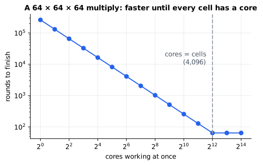
Reading it: both axes are logarithmic. Doubling the cores halves the time, a straight line, until the cores match the number of independent cells (the dashed line at 4,096). Past that point the line goes flat: more cores cannot help a problem that has run out of independent work. A small matrix leaves a big GPU mostly idle.
In code: counted_matmul multiplies with plain loops and counts every multiply and add; matmul_flops is the 2·m·n·k formula; parallel_rounds is the rounds formula above.
Why it matters in practice. A GPU is fast only when it is given a lot of
independent work at once: large matrices, and many sequences processed
together. That is why serving systems batch requests together
(primer.ml.inference) and why a small model answering one user at a time
uses a sliver of the chip. It is also why neural networks look the way they
do: architectures that turn into a few big matrix multiplies (the
transformer, primer.ml.transformer) won partly because they suit this
hardware, while step-by-step recurrences (primer.ml.cnn_rnn) do not.
2. The memory hierarchy: near is small, far is big
Everyday picture. Back in the kitchen. A cook's hands hold one or two things (the registers). The cutting board holds a few more (the on-chip SRAM, fast memory built into the chip itself). The fridge in the kitchen holds the day's ingredients (HBM, "high-bandwidth memory", the GPU's main memory). The storeroom down the hall is the CPU's memory (host memory). The warehouse across town is the disk. And other restaurants' pantries, reached by courier, are other machines over the network. Every step further out holds more and takes longer to reach. The cooks are fast; what slows the kitchen down is fetching.
Tiny worked example. Round, illustrative numbers for one datacenter GPU and the machine around it (orders of magnitude, not any product's specification):
| Level | Holds about | Moves about | Streaming 1 GB takes | What lives there |
|---|---|---|---|---|
| registers | 20 MB (across the chip) | 100 TB/s | 0.01 ms | the numbers being multiplied this instant |
| on-chip SRAM | 50 MB | 20 TB/s | 0.05 ms | tiles of the current multiply (section 3) |
| HBM | 80 GB | 3.35 TB/s | 0.30 ms | weights, activations, the KV cache |
| host memory | 1 TB | 50 GB/s (over the link to the GPU) | 20 ms | data waiting to be loaded, offloaded state |
| local disk | 10 TB | 10 GB/s | 100 ms | datasets, checkpoints |
| network | the whole cluster | 50 GB/s per GPU | 20 ms | other GPUs' gradients, remote storage |
Registers and SRAM never hold a whole gigabyte; the column shows their rate. Notice the jump from HBM to host memory: about 67 times slower. A GPU that has to reach past its own HBM is a cook walking to the storeroom for every carrot.
Level 3: the formula and its symbols
$$ t = \frac{\text{bytes}}{\text{bandwidth}} $$
Symbols
| Symbol | Meaning here | Units |
|---|---|---|
| $t$ | time to stream the data, ignoring the fixed delay before the first byte arrives (latency) | seconds |
| bytes | how much data moves | bytes (1 GB = 10⁹) |
| bandwidth | how many bytes per second the level can deliver | bytes per second |
In words: "the time to move data is its size divided by the speed of the pipe it moves through."
With the numbers: an 8-billion-parameter model at 2 bytes per
parameter is 16 GB. Reading it once from HBM takes 16 × 10⁹ / 3.35 × 10¹² =
4.78 ms: exactly the lower bound on time per generated token in
primer.ml.inference, because generating one token reads every weight once.
From host memory it would take 320 ms.
Level 3: in Python
In Python:
HBM, host = 3.35e12, 50e9
weights = 16e9
# t = bytes / bandwidth, in milliseconds
round(weights / HBM * 1000, 2)  # → 4.78
round(weights / host * 1000)  # → 320
# how many times slower the storeroom is than the fridge
round(HBM / host)  # → 67
flowchart LR
  ALU["arithmetic units"] <--> R["registers<br/>~20 MB, ~100 TB/s"]
  R <--> S["on-chip SRAM<br/>~50 MB, ~20 TB/s"]
  S <--> H["HBM<br/>~80 GB, ~3.35 TB/s"]
  H <--> D["host memory<br/>~1 TB, ~50 GB/s"]
  D <--> K["local disk<br/>~10 TB, ~10 GB/s"]
  H <--> N["network: other machines<br/>~50 GB/s per GPU"]
Reading it: start at the arithmetic units on the left and walk outward. Every box to the right is bigger and slower. The arithmetic units can only work on numbers in registers, so every number used must travel the whole way in from wherever it lives. The network hangs off HBM because fast clusters let a GPU send and receive data straight from its own memory without a detour through the CPU.
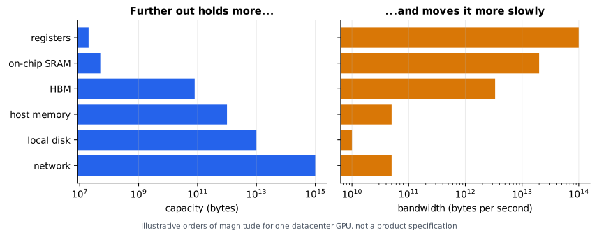
Reading it: the same six levels, top to bottom, on logarithmic axes. On the left, capacity climbs from megabytes to a petabyte. On the right, bandwidth falls from a hundred terabytes per second to ten gigabytes per second. The one place the order bends is the last two rows: a datacenter network is built to rival a local disk, so fetching from a nearby machine can be as fast as reading your own drive. Both are still around a hundred times slower than HBM.
In code: MEMORY_HIERARCHY lists the six levels with their capacity and bandwidth; transfer_seconds is the formula above.
Why it matters in practice. A model runs at full speed only if everything it touches every step (weights, activations, KV cache) lives in HBM. Spilling to host memory ("offloading") makes a model fit, at the price of each step waiting tens of times longer. And because HBM itself is slow compared with the arithmetic, the fastest code is the code that makes each trip to HBM count, which is the next section.
3. Arithmetic intensity: why data movement dominates
Everyday picture. A sandwich shop. If the cook walks to the storeroom for each slice of bread for each sandwich, the cook spends the day walking. If the cook carries a tray of bread and a tray of fillings to the bench and makes a batch of sandwiches from them, every trip feeds many sandwiches. Same sandwiches (FLOPs), far fewer trips (bytes). The ratio of the two is the arithmetic intensity: operations done per byte fetched.
Our imaginary GPU does 10¹⁵ FLOPs per second but reads only 3.35 × 10¹²
bytes per second from HBM, so it breaks even at about 299 FLOPs per
byte (the ridge point of the roofline in primer.ml.inference). Any work
doing fewer operations than that for each byte it fetches leaves the
arithmetic units waiting on memory.
Tiny worked example. Multiply two 4 × 4 matrices: 2 × 4³ = 128 FLOPs. Count the numbers fetched from slow memory (HBM) into fast memory (SRAM):
| Strategy | Numbers read | Numbers written | FLOPs per number moved |
|---|---|---|---|
| no reuse: each cell fetches its own row of A and column of B | 16 × (4 + 4) = 128 | 16 | 128 / 144 = 0.89 |
| 2 × 2 tiles: load a tile of A and a tile of B, use each number twice | 64 | 16 | 128 / 80 = 1.6 |
| one 4 × 4 tile: load everything once | 32 | 16 | 128 / 48 = 2.7 |
The arithmetic is identical in all three rows. Only the traffic changes. This trick is tiling: bring a small block of each matrix into fast memory and do every multiplication that block takes part in before throwing it away.
Level 3: the formula and its symbols
$$ \text{reads} = \frac{2\,n^3}{T} \qquad I = \frac{2\,n^3}{b\left(\dfrac{2\,n^3}{T} + n^2\right)} \approx \frac{T}{b} $$
Symbols
| Symbol | Meaning here | In the example |
|---|---|---|
| $n$ | both matrices are $n \times n$ | 4, then 4,096 |
| $T$ | tile width: fast memory works on $T \times T$ blocks | 1, 2, 4, then 128 |
| $2\,n^3$ | the FLOPs of the whole multiply (section 1, with $m = n = k$) | 128 |
| reads | numbers fetched from slow memory | 128, 64, 32 |
| $n^2$ | numbers written back: each answer cell once | 16 |
| $b$ | bytes per number: 2 at 16-bit, 1 at 8-bit | 2 |
| $I$ | arithmetic intensity: FLOPs per byte moved | FLOPs/byte |
| $\approx$ | "roughly", once $n$ is much bigger than $T$ and the writes are negligible |
In words: "every number fetched is used T times, so the traffic falls in proportion to the tile width, and the intensity rises in proportion to it."
With the numbers: for n = 4, the reads are 2 × 64 / T = 128, 64 and 32 for tiles of 1, 2 and 4, as the table says. For two 4096 × 4096 matrices in 16-bit with 128-wide tiles, I ≈ 128 / 2 = 64, and 63.0 once the writes are counted. In 8-bit the same tiles give 126: halving the bytes per number doubles the intensity.
Level 3: in Python
In Python:
n = 4
# reads = 2n³ / T, for tiles of 1, 2 and 4
[2 * n**3 // T for T in (1, 2, 4)]  # → [128, 64, 32]
def intensity(n, T, b):
    flops = 2 * n**3
    # bytes moved: every read, plus one write per answer cell
    moved = b * (2 * n**3 / T + n**2)
    return flops / moved
round(intensity(4096, 128, 2), 1)  # → 63.0
round(intensity(4096, 128, 1), 1)  # → 126.0
flowchart LR
  subgraph HBM["HBM: big, slow"]
    A["A, in T × T tiles"]
    B["B, in T × T tiles"]
    C["C, the answer"]
  end
  subgraph SRAM["on-chip SRAM: small, fast"]
    a["one tile of A"]
    b["one tile of B"]
    acc["running total for<br/>one T × T tile of C"]
  end
  A -- "load" --> a
  B -- "load" --> b
  a --> mm["multiply-add:<br/>T³ steps, no traffic"]
  b --> mm
  mm --> acc
  mm -. "next pair of tiles along k" .-> A
  acc -- "write once, at the end" --> C
Reading it: the left box is slow memory, the right box fast memory. For one tile of the answer, the kernel repeatedly loads one tile of A and one tile of B, does all T³ multiply-adds between them without touching slow memory, and adds the results into a running total that stays on chip. Only when the whole row of tiles has been consumed does it write the finished answer tile back, once. Fast memory never holds more than three tiles.
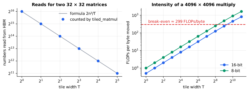
Reading it: on the left, dots are reads counted by actually running the tiled multiply on 32 × 32 matrices, and the line is the formula 2n³/T; they agree exactly, and each doubling of the tile halves the traffic. On the right, the intensity of a 4096 × 4096 multiply climbs with the tile width, and the dashed line is the chip's break-even point of 299. In 16-bit the tiles need to be about 650 wide to cross it. Three 650 × 650 tiles in 16-bit take about 2.5 MB, more fast memory than one group of cores has to itself, which is why real kernels tile at several levels at once (tiles in registers inside tiles in SRAM) and why lower-precision numbers, which shift the whole curve up, are so attractive.
The same idea runs through the rest of this primer:
- FlashAttention (
primer.ml.attention) tiles attention: blocks of queries, keys and values are loaded into SRAM, and the n × n score matrix is never written to HBM at all. Same answer, a fraction of the traffic. - Kernel fusion: adding a bias or applying an activation does about one FLOP per number it reads, hopelessly below 299, so these steps are done inside the matrix-multiply kernel while the tile is still on chip.
- Decode (
primer.ml.inference): generating one token for one user reads every weight to do just 2 FLOPs with it, an intensity of about 1. Batching users together is tiling across requests: one read of a weight serves every sequence in the batch.
In code: tiled_matmul runs the tiled multiply and returns a Traffic count of reads, writes, FLOPs and peak fast-memory use; matmul_reads and matmul_intensity are the formulas; primer.ml.inference.ridge_point is the break-even.
Why it matters in practice. Before asking how many FLOPs a piece of work needs, ask how many bytes it moves and how often each byte is reused. Most large speed-ups in modern AI systems (FlashAttention, fused kernels, batching, quantization) change the bytes, not the FLOPs.
4. Number formats: how many bits each number gets
Everyday picture. Scientific notation on a form with a fixed number of boxes: 6.02 × 10²³. One box holds the sign. A few boxes hold the power of ten, which sets how big or small the number can be: its range. The rest hold the digits, which set how finely it is measured: its precision. With a fixed number of boxes, moving a box from the digits to the power buys range and costs precision. Computers do the same with bits and powers of two, and call the parts the sign, the exponent and the mantissa (the stored digits).
Tiny worked example. Store −6.5 in bf16 ("brain float 16": 1 sign bit, 8 exponent bits, 7 mantissa bits).
- Sign: negative, so the sign bit is 1.
- Power of two: the largest power of two not above 6.5 is 4 = 2², so 6.5 = 1.625 × 2².
- Exponent: stored with a bias of 127 added, so that negative powers need no sign of their own: 2 + 127 = 129 = 10000001 in binary.
- Mantissa: the leading 1 of 1.625 is always there, so it is not stored. The fraction 0.625 = ½ + ⅛ is 0.101 in binary, padded to seven bits: 1010000.
- The 16 bits: 1 10000001 1010000.
Most numbers are not so lucky. 0.1 has no finite binary expansion, so it is rounded to the nearest value each format can hold: 0.10000000149 in fp32, 0.1000977 in bf16, 0.0999756 in fp16 and 0.1015625 in 8-bit E4M3.
Level 3: the formula and its symbols
$$ x = (-1)^{s} \times 2^{\,e - \text{bias}} \times \left(1 + \frac{f}{2^{M}}\right), \qquad \text{bias} = 2^{E-1} - 1 $$
Symbols
| Symbol | Meaning here | In the example |
|---|---|---|
| $s$ | the sign bit: 0 positive, 1 negative | 1 |
| $(-1)^s$ | −1 multiplied by itself $s$ times: +1 when $s = 0$, −1 when $s = 1$ | −1 |
| $E$ | how many exponent bits the format has | 8 |
| $e$ | the stored exponent, read as an ordinary whole number | 129 |
| bias | the offset subtracted from $e$, so stored values 1…254 stand for powers −126…127 | 127 |
| $M$ | how many mantissa bits the format has | 7 |
| $f$ | the stored mantissa, read as a whole number from 0 to $2^M - 1$ | 1010000 = 80 |
| $1 + f/2^M$ | the significand: the hidden leading 1 plus the stored fraction, between 1 and 2 | 1 + 80/128 = 1.625 |
| $x$ | the number the bits stand for | −6.5 |
In words: "the sign says plus or minus, the exponent says which power of two to scale by, and the mantissa says how far between that power and the next one the number sits."
With the numbers: (−1)¹ × 2^(129 − 127) × (1 + 80/128) = −1 × 4 × 1.625 = −6.5.
Level 3: in Python
In Python:
x = -6.5
M, bias = 7, 127
# s: 1 for a negative number
s = 1 if x < 0 else 0
# e: the power of two below |x| is 2², stored with the bias added
e = 2 + bias
e, format(e, "08b")  # → (129, '10000001')
# f: the fraction after the hidden 1 of |x| / 2², as a 7-bit whole number
f = round((abs(x) / 2**2 - 1) * 2**M)
f, format(f, "07b")  # → (80, '1010000')
# decode: (-1)^s × 2^(e - bias) × (1 + f / 2^M)
(-1)**s * 2**(e - bias) * (1 + f / 2**M)  # → -6.5
Two corners of the formula matter in practice. When the stored exponent is 0, the hidden 1 is dropped and the number is a subnormal: it lets values fade gradually towards zero instead of dropping off a cliff, at the cost of fewer significant bits. And IEEE-style formats reserve the all-ones exponent for infinity and NaN ("not a number"), which is where overflowing values go.
flowchart LR
  X["x = −6.5"] --> S["sign: negative<br/>s = 1"]
  X --> P["largest power of two<br/>not above 6.5: 2² = 4"]
  P --> E["exponent: 2 + bias 127<br/>e = 129 = 10000001"]
  P --> F["6.5 / 4 = 1.625<br/>drop the leading 1: .625"]
  F --> R["round .625 to 7 bits<br/>f = 1010000"]
  S --> B["1 | 10000001 | 1010000"]
  E --> B
  R --> B
Reading it: a number enters on the left and splits three ways. The sign is read off directly. The exponent comes from finding which pair of powers of two the number sits between. The mantissa is where the number sits within that pair, rounded to however many bits the format allows: this rounding box is the only place information is lost, and it is where every format differs.
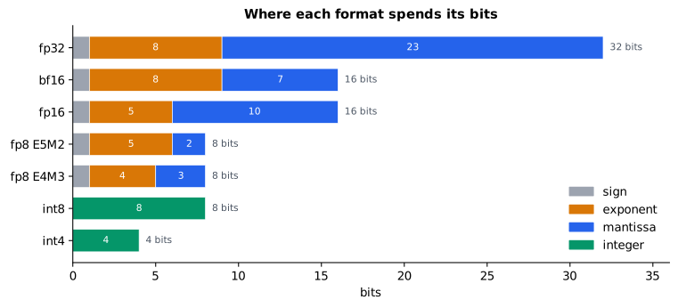
Reading it: each row is one format drawn to scale, one cell per bit,
with the sign in grey, the exponent in orange and the mantissa in blue.
Compare bf16 and fp16: the same 16 bits, split differently. bf16 is
literally the top half of fp32, keeping all 8 exponent bits (fp32's whole
range) and giving up precision; fp16 keeps more precision and gives up
range. The integer formats at the bottom have no exponent at all: every
value is a whole number, turned into a weight by one shared scale
(primer.ml.inference builds int8 and int4 quantization from scratch).
| Format | Bits (sign, exponent, mantissa) | Largest | Smallest at full precision | Gap just above 1 | Typical use |
|---|---|---|---|---|---|
| fp32 | 1, 8, 23 | 3.4 × 10³⁸ | 1.2 × 10⁻³⁸ | 1.2 × 10⁻⁷ | master weights, optimizer state, running sums |
| bf16 | 1, 8, 7 | 3.4 × 10³⁸ | 1.2 × 10⁻³⁸ | 1/128 ≈ 0.0078 | training and inference matrix multiplies |
| fp16 | 1, 5, 10 | 65,504 | 6.1 × 10⁻⁵ | 1/1024 ≈ 0.00098 | inference; training with loss scaling |
| fp8 E5M2 | 1, 5, 2 | 57,344 | 6.1 × 10⁻⁵ | 0.25 | gradients in 8-bit training |
| fp8 E4M3 | 1, 4, 3 | 448 | 0.0156 | 0.125 | weights and activations in 8-bit |
| int8 | 8-bit integer | 127 × scale | evenly spaced | none: a fixed step | quantized weights |
| int4 | 4-bit integer | 7 × scale | evenly spaced | none: a fixed step | quantized weights |
E4M3 bends the IEEE rules: it has no infinity, and spends that exponent on ordinary numbers instead, which is how 8 bits reach 448 rather than 240.
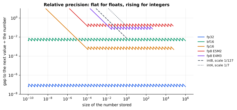
Reading it: the x-axis is the size of the number being stored; the y-axis is the gap to the next storable value, as a fraction of the number (lower is more precise); both are logarithmic. Each float format is a flat band: its relative precision is the same for tiny and huge numbers, which is the whole point of an exponent. The band's width is the range: it stops on the right at the largest value (65,504 for fp16, 448 for E4M3) and rises on the left where subnormals run out of bits. fp32 and bf16 are flat across the whole plot and far beyond it. The integer formats, here with a scale that maps 1.0 to the top code, are straight rising lines: their step is the same size everywhere, so small numbers get coarse, which is why quantized models use one scale per row or block of weights.
What the picture means for training (primer.ml.pretraining covers mixed
precision in full):
- Range failures. A gradient of 10⁻⁸ becomes exactly 0 in fp16 (below its smallest subnormal) but survives in bf16 as 1.0012 × 10⁻⁸. fp16 training therefore multiplies the loss by a large constant (loss scaling) to lift gradients into range; bf16 training does not need to.
- Precision failures. In bf16, 1 + 0.001 rounds back to exactly 1: a small weight update simply vanishes. So training keeps a master copy of the weights in fp32, adds its sums up in fp32, and uses 16-bit (or 8-bit) only for the big multiplies. That split is mixed precision.
Why smaller formats multiply throughput
Fewer bits per number pays three times:
- Bytes. Half the bytes per number moves twice the numbers per second
through every level of section 2, and fits twice the parameters in HBM.
Memory-bound work speeds up directly: the lower bound on time per token
for a 70-billion-parameter model (
primer.ml.inference) is 41.8 ms at 16-bit, 20.9 ms at 8-bit and 10.4 ms at 4-bit. - Intensity. The same tile does twice the FLOPs per byte (section 3: 63 becomes 126), pushing more work past the break-even point.
- Silicon. A multiplier is the expensive part of the chip, and its size grows with the square of the number of significand bits.
Everyday picture. Long multiplication by hand: multiplying two 3-digit numbers means writing a 3 × 3 grid of single-digit products; two 6-digit numbers need a 6 × 6 grid, four times the work. A chip's multiplier is that grid built in wires.
Level 3: the formula and its symbols
$$ \text{cells} = p^{2}, \qquad p = M + 1 $$
Symbols
| Symbol | Meaning here | In the example |
|---|---|---|
| $M$ | stored mantissa bits | 23, 10, 7, 3 |
| $p$ | significand bits: the stored mantissa plus the hidden leading 1 | 24, 11, 8, 4 |
| cells | one-bit products in a schoolbook (array) multiplier: one per pair of bits |
In words: "multiplying two p-bit significands needs one small cell for every pair of bits, so p times p cells; the exponents only need adding, which is cheap."
With the numbers: fp32 needs 24² = 576 cells, fp16 11² = 121, bf16 8² = 64, and fp8 E4M3 4² = 16: one fp32 multiplier's worth of silicon holds many 8-bit ones. Accelerators typically list roughly double the peak operations per second each time the format halves.
Level 3: in Python
In Python:
# stored mantissa bits for fp32, fp16, bf16 and fp8 E4M3
mantissa_bits = [23, 10, 7, 3]
# p = M + 1, and cells = p²
[(M + 1) ** 2 for M in mantissa_bits]  # → [576, 121, 64, 16]
In code: FloatFormat describes a format by its exponent and mantissa bits, with FloatFormat.max_value, FloatFormat.min_normal, FloatFormat.min_subnormal and FloatFormat.epsilon derived from them; FP32, BF16, FP16, FP8_E5M2 and FP8_E4M3 are the five formats; encode rounds a number into its three fields with plain arithmetic, decode turns fields back into a number, round_to does both, and bit_string prints the bits; multiplier_cells is the p² formula. The tests check round_to against NumPy's own float16 and float32.
Why it matters in practice. Picking a number format is picking a point on the range-versus-precision curve for each kind of number in a model. Weights and activations tolerate coarse formats; gradients need range; the running sums of long dot products need precision. Modern training and serving use a different format for each, and the savings are among the largest in the field.
5. Many GPUs: the cost of talking
Everyday picture. A group project. Four people each work through a quarter of the exercises, and then must agree on one combined answer sheet. Sitting at the same table they can compare notes in seconds; living in different cities they must post letters. The more often a team must compare notes, the more it matters who sits at the same table.
Large models are trained on many GPUs because no single one has the memory or the speed. The simplest split is data parallelism: every GPU holds a copy of the model and works on different examples, and after each step their gradients must be added up, so every copy takes the same step. That "add up, and give everyone the total" operation is an all-reduce.
Tiny worked example: a ring all-reduce. Four GPUs each hold a gradient of 8 numbers. Each splits its gradient into 4 chunks of 2 numbers and they sit in a ring, each passing to its right-hand neighbour.
- Reduce-scatter, 3 steps: each GPU sends one chunk to its neighbour, which adds it to its own copy of that chunk. After 3 steps, each GPU holds one chunk that contains the sum from all four.
- All-gather, 3 more steps: the finished chunks travel round the ring, overwriting the stale copies.
Each GPU sent 6 chunks of 2 numbers, 12 numbers, which is 2 × 3/4 × 8. The remarkable part: with 400 GPUs instead of 4, each would still send just under twice its gradient. The work per GPU barely grows.
flowchart LR
  G0["GPU 0<br/>chunks a b c d"] -- "one chunk per step" --> G1["GPU 1<br/>chunks a b c d"]
  G1 -- "one chunk per step" --> G2["GPU 2<br/>chunks a b c d"]
  G2 -- "one chunk per step" --> G3["GPU 3<br/>chunks a b c d"]
  G3 -- "one chunk per step" --> G0
Reading it: four GPUs in a ring, each only ever talking to its right-hand neighbour. Every link is busy at every step, each carrying a different chunk, so no link sits idle and no single GPU becomes a bottleneck. After 2 × (4 − 1) = 6 steps, every GPU has every chunk summed over all four.
Level 3: the formula and its symbols
$$ t_{\text{all-reduce}} = \frac{2\,(N-1)}{N} \cdot \frac{S}{B} \qquad t_{\text{compute}} = \frac{6\,P\,D}{F} $$
Symbols
| Symbol | Meaning here | In the example |
|---|---|---|
| $N$ | GPUs taking part | 8 |
| $S$ | bytes of gradient each GPU holds | 7 × 10⁹ parameters × 2 bytes = 14 GB |
| $B$ | each GPU's link bandwidth | 500 GB/s in one machine, 50 GB/s between machines (illustrative) |
| $\frac{2(N-1)}{N}$ | the fraction of its gradient each GPU sends in a ring all-reduce: just under 2 | 1.75 |
| $P$ | parameters in the model | 7 × 10⁹ |
| $D$ | tokens each GPU processes per step | 16,384 |
| $6$ | FLOPs per parameter per token in training: 2 forward, 4 backward | |
| $F$ | the GPU's arithmetic speed | 10¹⁵ FLOPs per second |
In words: "talking takes just under twice the gradient's size divided by the link speed, however many GPUs there are; computing takes six operations per parameter per token, divided by the chip's speed."
With the numbers: inside one machine, 1.75 × 14 × 10⁹ / 500 × 10⁹ = 49 ms. Across machines, 490 ms. The arithmetic for the step is 6 × 7 × 10⁹ × 16,384 / 10¹⁵ = 0.69 s. Inside a machine, talking costs 7% of the computing time; across machines, 71%.
Level 3: in Python
In Python:
N, S = 8, 14e9
in_machine, between_machines = 500e9, 50e9
# 2(N - 1)/N × S / B, in milliseconds
round(2 * (N - 1) / N * S / in_machine * 1000)  # → 49
round(2 * (N - 1) / N * S / between_machines * 1000)  # → 490
P, D, F = 7e9, 16_384, 1e15
# 6·P·D / F, in seconds
round(6 * P * D / F, 2)  # → 0.69
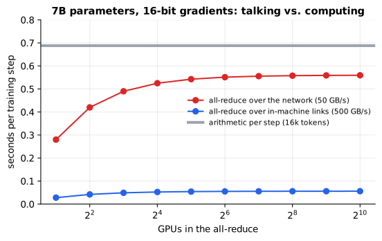
Reading it: the x-axis is the number of GPUs (log scale); the y-axis is seconds per training step. The flat grey line is the arithmetic every GPU does per step. The two rising curves are the all-reduce over each kind of link, and both flatten out almost at once: that is the ring's 2(N − 1)/N approaching 2. The gap between the curves is the whole story: the same gradient costs ten times more over the network than over in-machine links, bringing communication close to the cost of the arithmetic itself. Real systems hide part of it by sending the gradients of later layers while earlier layers are still computing theirs.
flowchart TB
  subgraph M1["machine 1: fast links, ~500 GB/s"]
    a1["GPU"] <--> a2["GPU"] <--> a3["GPU"] <--> a4["GPU"]
  end
  subgraph M2["machine 2: fast links, ~500 GB/s"]
    b1["GPU"] <--> b2["GPU"] <--> b3["GPU"] <--> b4["GPU"]
  end
  M1 <-- "network, ~50 GB/s per GPU:<br/>data parallelism, once per step" --> M2
  TP["tensor parallelism:<br/>talks inside every layer"] -.-> M1
  TP -.-> M2
Reading it: two machines, each with a few GPUs joined by fast links, and
a slower network between them. The chattiest kind of splitting, tensor
parallelism (cutting each matrix multiply across GPUs, which must swap
partial results inside every layer), is kept within one machine's fast
links. Kinds that talk rarely, like data parallelism (one all-reduce per
step) and pipeline parallelism (passing activations only between
neighbouring stages of layers), span the slower network. The layout of the
wires decides the layout of the work. primer.ml.pretraining builds these
strategies in full.
In code: ring_all_reduce simulates the ring step by step and counts the numbers each GPU sends; all_reduce_seconds and training_step_seconds are the two formulas; IN_MACHINE_LINK and BETWEEN_MACHINES_LINK are the illustrative link speeds.
Why it matters in practice. At scale, a cluster's network matters as much as its chips. Parallelism strategies are chosen by matching how often each kind talks to how fast each link is, and a training run that ignores the map spends its budget waiting.
6. Will it fit? Memory math for serving
Everyday picture. A bookshelf of fixed width. The encyclopedia (the model's weights) must go on it, whole. Whatever space is left holds one notebook per customer being served (their KV cache), and a notebook grows with every word of the conversation. Thinner volumes, printed in a smaller number format, leave room for more notebooks.
Tiny worked example. A model shaped like Llama 3 70B (80 layers, 8
key/value heads of 128 dimensions each) on one 80 GB GPU. Its KV cache
costs 2 × 80 × 8 × 128 × 2 = 327,680 bytes per token at 16-bit
(primer.ml.inference derives this).
| Weights | Weight memory | Left for the cache | Tokens of 16-bit cache | Tokens of 8-bit cache |
|---|---|---|---|---|
| 16-bit | 140 GB | none: does not fit | 0 | 0 |
| 8-bit (fp8) | 70 GB | 10 GB | 30,517 | 61,035 |
| 4-bit | 35 GB | 45 GB | 137,329 | 274,658 |
This ignores activations and the serving software's own working memory, which take several more gigabytes in practice.
Level 3: the formula and its symbols
$$ P \, b_w + C \times 2\,L\,H_{kv}\,d_h\,b_{kv} \le M_{\text{GPU}} $$
Symbols
| Symbol | Meaning here | In the example |
|---|---|---|
| $P$ | parameters | 7 × 10¹⁰ |
| $b_w$ | bytes per weight: bits ÷ 8 | 2, 1 or 0.5 |
| $C$ | tokens held in the KV cache, summed over every request being served | the unknown |
| $2$ | one key and one value per token | |
| $L$ | layers, each with its own cache | 80 |
| $H_{kv}$ | key/value heads | 8 |
| $d_h$ | dimensions per head | 128 |
| $b_{kv}$ | bytes per cached number | 2 or 1 |
| $M_{\text{GPU}}$ | the GPU's memory | 80 × 10⁹ bytes |
| $\le$ | "must be at most" |
In words: "the weights, plus every cached token's keys and values across every layer, must fit in the GPU's memory."
With the numbers: with fp8 weights, 7 × 10¹⁰ × 1 = 70 GB, leaving 10 GB. 10 × 10⁹ / 327,680 = 30,517 tokens of 16-bit cache, or 61,035 with the cache in fp8 too: one long conversation, or a dozen short ones.
Level 3: in Python
In Python:
P, M_gpu = 70e9, 80e9
L, H_kv, d_h = 80, 8, 128
def kv_per_token(b_kv):
    # a key and a value, per layer, per KV head
    return 2 * L * H_kv * d_h * b_kv
kv_per_token(2)  # → 327680
# weight GB at 16, 8 and 4 bits
[P * bits / 8 / 1e9 for bits in (16, 8, 4)]  # → [140.0, 70.0, 35.0]
# tokens of cache beside fp8 weights, with a 16-bit cache and then an fp8 one
int((M_gpu - P * 1) // kv_per_token(2)), int((M_gpu - P * 1) // kv_per_token(1))  # → (30517, 61035)
flowchart LR
  P["parameters × bytes per weight"] --> W["weights"]
  T["tokens × bytes per token"] --> K["KV cache"]
  W --> Q{"weights + cache<br/>fit in GPU memory?"}
  K --> Q
  Q -- yes --> Y["serve: spare room means<br/>more users or longer contexts"]
  Q -- no --> N["smaller formats, fewer KV heads,<br/>shorter contexts, or more GPUs"]
Reading it: two budgets feed one question. The weights are a fixed cost, set by the parameter count and the number format. The cache grows with every token of every active conversation. If they fit together, whatever is left over becomes capacity: more concurrent users, longer contexts. If they don't, every lever on the right shrinks one of the two inputs, or splits the model across GPUs joined by the fast links of section 5.
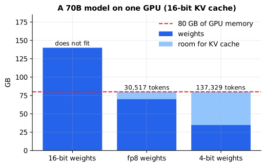
Reading it: each bar is one choice of weight format for the same 70-billion-parameter model. The dark part is the weights; the light part is the room left for the KV cache, labelled with how many 16-bit tokens fit in it. The dashed line is the GPU's 80 GB. At 16-bit the weights alone break through the line. Each halving of the weight format frees memory that turns directly into tokens of cache, which is to say into users.
In code: max_cache_tokens subtracts the weights and divides what is left by the per-token cache, using primer.ml.inference.weight_bytes and primer.ml.inference.kv_cache_bytes_per_token; LLAMA3_70B_SHAPE holds the example model's shape.
Why it matters in practice. This arithmetic comes first in every
deployment: the number format sets whether a model fits, how many users
share a GPU, and (because decode reads every weight per token) how fast
each of them sees words appear. primer.ml.inference carries it on into
batching, speculative decoding and prompt caching.
In 20 seconds
- GPUs are thousands of simple cores doing the same step on different numbers. Matrix multiplies (2·m·n·k FLOPs, every cell independent) are the perfect workload, as long as there is enough independent work.
- Memory hierarchy: registers, on-chip SRAM, HBM, host memory, disk, network. Each step out is bigger and slower; the GPU runs at full speed only on data in HBM or closer.
- Arithmetic intensity: the chip does hundreds of operations in the time it fetches one byte, so speed is set by bytes moved. Tiling reuses each fetched number T times and cuts traffic T-fold; FlashAttention, kernel fusion and batching are the same idea.
- Number formats: sign, exponent (range) and mantissa (precision). bf16 keeps fp32's range with less precision; fp16 the reverse; fp8 and int8/int4 trade more. Fewer bits means fewer bytes, higher intensity and smaller multipliers, so throughput roughly doubles per halving.
- Many GPUs: a ring all-reduce costs about 2 × gradient size ÷ link speed, whatever the GPU count. Chatty parallelism stays on fast in-machine links; the rest crosses the network.
- Serving: weights plus KV cache must fit; the number format decides both what fits and how fast each token comes.
Self-test questions
Why are GPUs, rather than CPUs, used to train and run neural networks? Nearly all of a network's work is matrix multiplication, where every output cell is an independent dot product. A GPU spends its silicon on thousands of simple arithmetic units (plus matrix units) that apply the same instruction to different numbers, so it can compute thousands of cells at once. A CPU spends its silicon on a few flexible cores that are better at branchy, sequential code.
How many FLOPs does multiplying a 1,000 × 2,000 matrix by a 2,000 × 500 matrix take, and why that formula? 2 × 1,000 × 500 × 2,000 = 2 × 10⁹. There are m·n = 500,000 output cells, each a dot product of length k = 2,000, and each step of a dot product is one multiply and one add.
The chip can do 10¹⁵ FLOPs per second but a model runs far slower. What is usually the bottleneck, and how do you tell? Memory bandwidth. Compare the work's arithmetic intensity (FLOPs per byte moved from HBM) with the chip's break-even ratio, peak FLOPs divided by bandwidth (about 299 here). Below it, the arithmetic units wait on memory; generating one token for one user has an intensity near 1, so it is deeply memory-bound.
How does tiling a matrix multiply reduce memory traffic, and what limits it? Each block of numbers is loaded into fast on-chip memory once and used for every multiplication it takes part in, T times, instead of being fetched again for each one. Reads fall from 2n³ to 2n³/T. The limit is fast-memory size: three T × T tiles must fit at once, so real kernels tile at several levels of the hierarchy.
What is the difference between bf16 and fp16, and why do many training runs prefer bf16? Both have 16 bits. bf16 has fp32's 8 exponent bits and 7 mantissa bits: the same range as fp32, less precision. fp16 has 5 exponent bits and 10 mantissa bits: more precision, but a range that tops out at 65,504 and rounds gradients smaller than about 3 × 10⁻⁸ to zero. bf16 avoids the need for loss scaling; its coarse precision is handled by keeping fp32 master weights and fp32 sums.
Why does halving the bits per number roughly double throughput? Three reasons: half the bytes to move, so memory-bound work runs twice as fast and twice the parameters fit; twice the FLOPs per byte for the same tile, so more work clears the break-even point; and multipliers whose area grows with the square of the significand bits, so many more small multipliers fit in the same silicon.
Why is tensor parallelism usually kept inside one machine while data parallelism spans many? Tensor parallelism splits every matrix multiply, so GPUs must exchange partial results inside every layer, many times per step: it needs the fast in-machine links. Data parallelism communicates once per step (an all-reduce of the gradients), which a ring spreads so each GPU sends only about twice its gradient, and which can overlap with the backward pass, so it tolerates the slower network.
Will a 70-billion-parameter model serve from one 80 GB GPU? Not in 16-bit: the weights alone are 140 GB. In 8-bit the weights take 70 GB, leaving about 10 GB, around 30,000 tokens of 16-bit KV cache for a model with 80 layers and 8 KV heads of 128 dimensions. In 4-bit, 45 GB is left, about 137,000 tokens. Leave headroom for activations and the serving software.
The papers behind this lesson
- Williams, Waterman and Patterson, Roofline: An Insightful Visual Performance Model for Multicore Architectures (2009): https://doi.org/10.1145/1498765.1498785. Introduced the roofline: judge a kernel by its arithmetic intensity against the machine's balance of compute and bandwidth.
- Dao et al., FlashAttention: Fast and Memory-Efficient Exact Attention with IO-Awareness (2022): https://arxiv.org/abs/2205.14135. Applied tiling to attention so the score matrix never reaches HBM, showing that counting memory traffic rather than FLOPs is what makes attention fast. Annotated companion
- Micikevicius et al., Mixed Precision Training (2017): https://arxiv.org/abs/1710.03740. Showed that networks train in 16-bit floats with fp32 master weights, fp32 accumulation and loss scaling.
- Kalamkar et al., A Study of BFLOAT16 for Deep Learning Training (2019): https://arxiv.org/abs/1905.12322. Showed that bf16, with fp32's range, trains a wide range of models to fp32 quality without loss scaling.
- Micikevicius et al., FP8 Formats for Deep Learning (2022): https://arxiv.org/abs/2209.05433. Proposed the E4M3 and E5M2 8-bit formats and showed that training and inference hold up in them.
- Shoeybi et al., Megatron-LM: Training Multi-Billion Parameter Language Models Using Model Parallelism (2019): https://arxiv.org/abs/1909.08053. Split each transformer layer's matrix multiplies across the GPUs of one machine, the tensor parallelism of section 5. Annotated companion
- Sergeev and Del Balso, Horovod: fast and easy distributed deep learning in TensorFlow (2018): https://arxiv.org/abs/1802.05799. Brought the bandwidth-optimal ring all-reduce to deep learning training.
Further reading
- Horace He, Making Deep Learning Go Brrrr From First Principles: https://horace.io/brrr_intro.html
- How to Scale Your Model (a book on TPUs, GPUs and parallelism for transformers): https://jax-ml.github.io/scaling-book/
- Williams, Waterman and Patterson, Roofline (2009): https://doi.org/10.1145/1498765.1498785
- Dao et al., FlashAttention (2022): https://arxiv.org/abs/2205.14135
- Micikevicius et al., Mixed Precision Training (2017): https://arxiv.org/abs/1710.03740
- Micikevicius et al., FP8 Formats for Deep Learning (2022): https://arxiv.org/abs/2209.05433
- PyTorch automatic mixed precision: https://pytorch.org/docs/stable/amp.html
- NVIDIA, CUDA C++ Programming Guide (how one GPU family organises cores and memory): https://docs.nvidia.com/cuda/cuda-programming-guide/index.html
1r""" 2# The hardware underneath: chips, memory, links and number formats 3 4Run: `python -m primer.ml.hardware` 5 6New to the notation? `primer.notation` explains every symbol used here from 7zero. This lesson builds on the cost arithmetic of `primer.ml.inference`. 8 9## Level 1: The practitioner's guide 10 11**In one sentence.** The hardware under a model is thousands of simple 12multipliers starved by slow memory, so what you rent or buy is decided by 13bytes (does the model fit, how fast can its weights be read, how fast can 14chips talk) and the number format you store those bytes in is the cheapest 15lever you have. 16 17**When you need it.** You need this the day you have to pick a machine: a 18laptop for local experiments, a cloud GPU for a demo, a multi-GPU server 19for serving a 70-billion-parameter model, or a cluster for training. You 20also need it when a model runs far slower than its FLOP count suggests. The 21tell is a spec sheet you cannot read: teraFLOPS, HBM, NVLink, bf16, FP8, and 22no idea which number will bite. This lesson's imaginary datacenter GPU 23does about 10¹⁵ operations per second but reads only 3.35 TB/s, so any work 24doing fewer than about 299 operations per byte fetched leaves the 25multipliers idle; generating one token for one user does about 1. You do not 26need this lesson while you call a hosted API: the provider has done the 27sizing for you. You need it the moment the bill or the latency makes you 28consider doing it yourself. 29 30**Your options.** From the least hardware to the most, at what each can 31hold and how its parts talk: 32 33| Option | What it is | What fits, roughly | What it costs | Where it lives | 34|---|---|---|---|---| 35| A hosted API | Someone else's GPUs behind a per-token price | Any model they offer, at any scale | Money per token, no capacity planning, no control over the machine | The provider | 36| A laptop or consumer GPU | One chip with a few to a few tens of gigabytes of memory, no fast links | Small models, or larger ones quantized to 4 bits: an 8B model at 4 bits is 4 GB, a 70B is 35 GB (this lesson's memory math) | Cheap and private; slow per token, one user at a time | Your desk | 37| One datacenter GPU | 80 GB of HBM at 3.35 TB/s (NVIDIA's H100 SXM specification, and this lesson's constants) | A 70B model only at 8 bits (70 GB, 10 GB of cache left) or 4 bits (35 GB, 45 GB left); a 16-bit 70B does not fit | Rental by the hour; the whole card even when one user uses 0.3% of it | A cloud instance or a rack | 38| One machine, several GPUs on fast links | Chips joined at hundreds of GB/s (NVLink is 900 GB/s on an H100 SXM; this lesson models 500) | A model split across the GPUs, exchanging partial results inside every layer | Several cards' rent; the fast links are what you are paying for | A cloud instance or a rack | 39| Many machines over a network | Machines joined at tens of GB/s per GPU (this lesson models 50) | Training runs and fleets: each machine holds a copy or a slice, and they talk once per step | The most money and the most engineering; the network becomes the bottleneck | A cluster | 40 41**How to choose.** Start from the model's size in bytes and the number 42format you are willing to run it in. 43 44- Compute the weights first: parameters times bytes per weight. If they 45 fit in one GPU with room for the KV cache, stop there; one chip with no 46 links is the simplest system you can operate. 47- If they do not fit, drop the format before adding chips: 8-bit weights 48 halve the bytes and, on this lesson's numbers, cut the lower bound on 49 decode time for a 70B model from 41.8 ms to 20.9 ms per token, and 4-bit 50 to 10.4 ms. Check quality on your own tasks afterwards. 51- If they still do not fit, add GPUs inside one machine, where the links 52 are fast enough to split a layer across chips. 53- Cross to many machines only for training or for a fleet, and design the 54 split so that the chatty parallelism (tensor parallelism, talking inside 55 every layer) stays within a machine and only once-per-step traffic 56 crosses the network. 57- For training, pick bf16 for the multiplies and keep fp32 master weights: 58 a gradient of 10⁻⁸ becomes exactly 0 in fp16 but survives in bf16, and a 59 weight update of 0.001 vanishes in bf16 unless the master copy is fp32 60 (this lesson's format table). FP8 training is real and works on models up 61 to 175B parameters with no hyperparameter changes (Micikevicius et al., 62 *FP8 Formats for Deep Learning*), but it needs software that handles the 63 scaling for you. 64- Whatever you pick, measure what fraction of peak FLOPS you reach. If it 65 is 80%, you are at least 80% compute-bound; if it is a few percent, you are 66 moving bytes, and more arithmetic will not help (Horace He, *Making Deep 67 Learning Go Brrrr*). 68 69**What it costs.** Memory is the price of admission and bandwidth is the 70speed limit. Reading 16 GB of weights once takes 4.78 ms from HBM on this 71lesson's GPU, 320 ms from the host's memory, 67 times slower: a model 72"offloaded" to CPU memory runs, but each token waits that much longer. 73Formats set both bills: halving the bits halves the bytes moved, doubles the 74operations per byte a tiled kernel achieves (63 becomes 126 in this lesson's 754096 × 4096 example), and shrinks the multiplier itself (an fp32 multiplier 76needs 576 cells of silicon, an fp8 one 16), which is why accelerators list 77roughly double the peak throughput at each halving of the format (the H100 78lists 1,979 TFLOPS at bf16 and 3,958 at FP8, both with sparsity). What a 79format costs you in return is range or precision: fp16 tops out at 65,504, 80fp8 E4M3 at 448, and int4 holds only 15 levels, so small weights vanish 81without a per-row scale. Links cost time at scale: on this lesson's numbers 82an all-reduce of a 14 GB gradient across 8 GPUs takes 49 ms inside a machine 83and 490 ms across machines, against 690 ms of arithmetic per step, so the 84same run spends 7% of its time talking on fast links and 71% over a network. 85Power is part of the rent too: an H100 SXM is rated up to 700 W. 86 87**What breaks.** 88 89- **The model "fits" and then does not.** Weights are the fixed cost; the KV 90 cache grows with every token of every conversation, and activations and 91 the serving software take several more gigabytes. Size for weights plus 92 cache plus headroom, not weights alone. 93- **A big GPU idles on a small job.** A single user's decode reads every 94 weight to do two operations with it. Without batching, most of the card 95 you rent does nothing. 96- **fp16 training silently zeros gradients**: it loses precision below 97 6 × 10⁻⁵ and rounds anything under about 3 × 10⁻⁸ to zero (this lesson's 98 format table). Use loss scaling, or use bf16, which trains to fp32 99 quality with no hyperparameter changes (Kalamkar et al.). 100- **bf16 swallows small updates**: 1 + 0.001 rounds back to 1. Keep master 101 weights and long running sums in fp32. 102- **fp8 overflows**: 500 in E4M3 is not a number. The format needs per-tensor 103 scaling that the training or serving library supplies; do not cast by hand. 104- **Offloading to host memory** makes a model fit at the price of tens of 105 times slower steps. It is for experiments, not for serving. 106- **Tensor parallelism across a network** stalls in every layer. Keep it on 107 the fast links inside a machine. 108 109**In the wild.** NVIDIA's H100 specification gives the numbers this 110lesson rounds (80 GB at 3.35 TB/s, 900 GB/s NVLink). The formats each have a paper: Kalamkar et al. studied bf16 for training, 111and Micikevicius et al. proposed the two fp8 encodings, E4M3 and E5M2, and 112earlier the mixed-precision recipe (fp32 master weights, loss scaling) that 113PyTorch's automatic mixed precision, linked in Further reading, implements. 114The roofline model this lesson uses to decide 115memory-bound from compute-bound is Williams, Waterman and Patterson's, and 116FlashAttention (Dao et al.) is the best-known application of tiling to a 117model. Megatron-LM (Shoeybi et al.) is the tensor parallelism that lives on 118fast links, and Horovod (Sergeev and Del Balso) brought the ring all-reduce 119to deep learning. *How to Scale Your Model*, linked in Further reading, 120carries the same arithmetic through TPUs and GPUs to full training runs. 121 122**Go deeper.** Level 2 builds each number here from nothing: a matrix 123multiply counted by hand, a memory hierarchy with its six levels, a tiled 124multiply whose traffic you can watch fall, a 16-bit float encoded bit by bit 125and every format's range and precision derived from its bit widths, a ring 126all-reduce simulated on four GPUs, and the serving-fit table computed from 127the formulas. If you only needed to choose a machine and a format, you are 128done. 129 130## Level 2: How it works, from scratch 131 132Every lesson so far has counted operations: so many multiplies per token, 133so many parameters. This lesson looks at the machine that performs them, 134because the machine explains things the maths alone never will: why a model 135that "needs" a tenth of a millisecond of arithmetic takes five milliseconds 136per token, why training runs are spread across thousands of chips in a 137particular way, and why everyone is shrinking numbers from 32 bits to 8. 138 139Three facts carry the whole lesson: 140 1411. **A GPU is thousands of simple arithmetic units** doing the same step on 142 different numbers. Neural networks are mostly matrix multiplies, which 143 are exactly that kind of work. 1442. **Arithmetic is cheap; moving data is expensive.** The chip can multiply 145 far faster than its memory can feed it, so speed is usually decided by 146 how many bytes move, not how many operations run. 1473. **Fewer bits per number helps everywhere at once**: more numbers per 148 byte moved, more numbers in memory, and smaller, more numerous 149 multipliers on the chip. 150 151Sections 5 and 6 then apply those facts to many GPUs working together, and 152to the question every deployment starts with: will the model fit? 153 154## 1. Why GPUs: thousands of simple cooks 155 156**Everyday picture.** A CPU is a few master chefs. Each can cook anything, 157improvise, and follow a recipe full of "if the sauce splits, do this 158instead". A GPU is a kitchen of thousands of line cooks who all do the same 159step at the same moment on different ingredients: "everyone, chop your 160carrot now." That kitchen is useless for inventing a menu and unbeatable at 161ten thousand identical salads. A neural network is ten thousand identical 162salads: nearly all of its work is **matrix multiplication**, the same 163multiply-and-add done billions of times on different numbers. 164 165**Tiny worked example.** Multiply a 2 × 3 matrix by a 3 × 2 matrix: 166 167$$ 168A = \begin{pmatrix} 1 & 2 & 3 \\ 4 & 5 & 6 \end{pmatrix}, \quad 169B = \begin{pmatrix} 7 & 8 \\ 9 & 10 \\ 11 & 12 \end{pmatrix}, \quad 170AB = \begin{pmatrix} 58 & 64 \\ 139 & 154 \end{pmatrix} 171$$ 172 173**Symbols** 174 175| Symbol | Meaning here | Shape | 176|---|---|---| 177| $A$ | the left matrix: 2 rows of 3 numbers | 2 × 3 | 178| $B$ | the right matrix: 3 rows of 2 numbers | 3 × 2 | 179| $AB$ | the **matrix multiply**: the cell in row $i$, column $j$ is row $i$ of $A$ dotted with column $j$ of $B$ | 2 × 2 | 180| $\begin{pmatrix}\ldots\end{pmatrix}$ | a matrix written out, row by row | | 181 182**In words:** "each cell of the answer is one row of A times one column of 183B, multiplied position by position and added up." 184 185**With the numbers:** the top-left cell is 1·7 + 2·9 + 3·11 = 7 + 18 + 33 = 186**58**; the bottom-right is 4·8 + 5·10 + 6·12 = 32 + 50 + 72 = **154**. Each 187cell took 3 multiplies and 3 additions (each product added to a running 188total that starts at 0), so the 4 cells took 12 multiplies and 12 additions. 189The crucial detail: **no cell needs any other cell's answer.** Four cooks 190could take one cell each and finish at the same moment. 191 192**In Python:** 193 194```python 195A = [[1, 2, 3], [4, 5, 6]] 196B = [[7, 8], [9, 10], [11, 12]] 197m, k, n = len(A), len(B), len(B[0]) 198# each cell: row i of A dotted with column j of B 199[[sum(A[i][p] * B[p][j] for p in range(k)) for j in range(n)] for i in range(m)] # → [[58, 64], [139, 154]] 200``` 201 202That count generalises into the most useful formula in this lesson. A 203**FLOP** (floating-point operation) is one multiply or one add, and 204multiplying an m × k matrix by a k × n matrix costs: 205 206$$ 207\text{FLOPs} = 2\,m\,n\,k 208$$ 209 210**Symbols** 211 212| Symbol | Meaning here | In the example | 213|---|---|---| 214| $m$ | rows of the left matrix (and of the answer) | 2 | 215| $k$ | the shared inner size: columns of the left, rows of the right; the length of each dot product | 3 | 216| $n$ | columns of the right matrix (and of the answer) | 2 | 217| $m\,n$ | how many cells the answer has | 4 | 218| $2$ | one multiply plus one add per step of a dot product | | 219| FLOPs | floating-point operations in total | 24 | 220 221**In words:** "every one of the m·n answer cells is a dot product of length 222k, and every step of a dot product is a multiply and an add." 223 224**With the numbers:** 2 × 2 × 2 × 3 = **24** for the example. A 4096 × 4096 225by 4096 × 4096 multiply, the size of one weight matrix in a mid-sized model, 226costs 2 × 4096³ ≈ 1.37 × 10¹¹ FLOPs. At the 10¹⁵ FLOPs per second of the 227imaginary datacenter GPU used throughout `primer.ml.inference`, that is 228about 0.14 milliseconds, if the chip could be kept busy. 229 230**In Python:** 231 232```python 233m, n, k = 2, 2, 3 234# 2 FLOPs per step, k steps per cell, m·n cells 2352 * m * n * k # → 24 236flops = 2 * 4096 * 4096 * 4096 237flops # → 137438953472 238# milliseconds at 10¹⁵ FLOPs per second 239round(flops / 1e15 * 1000, 2) # → 0.14 240``` 241 242Hardware usually does "multiply, then add to a running total" as a single 243instruction, the **fused multiply-add**, which is why FLOPs come in pairs. 244 245```mermaid 246flowchart LR 247 subgraph CPU["CPU: a few master chefs"] 248 direction TB 249 c1["core: big control unit,<br/>big cache, runs any code"] 250 c2["core"] 251 c3["core"] 252 end 253 subgraph GPU["GPU: thousands of line cooks"] 254 direction TB 255 g1["group of cores:<br/>one instruction, many numbers"] 256 g2["group of cores"] 257 g3["... about a hundred groups"] 258 g4["matrix units: a small<br/>tile multiply per instruction"] 259 end 260 W["matrix multiply:<br/>m × n independent cells"] --> GPU 261 BR["branchy code:<br/>if this then that"] --> CPU 262``` 263 264**Reading it:** the two boxes spend their silicon differently. The CPU 265spends it on a few cores that each handle any instruction stream quickly, 266including code full of decisions. The GPU spends it on arithmetic: groups 267of cores that all execute the *same* instruction on *different* numbers, 268plus (on most modern accelerators) **matrix units** that multiply a small 269tile of numbers in one instruction. A matrix multiply is a perfect fit for 270the GPU, because its m × n cells are independent and identical in shape. 271 272How far does the independence go? Suppose each core takes whole cells and 273performs one multiply-add per round: 274 275$$ 276\text{rounds} = \left\lceil \frac{m\,n}{\text{cores}} \right\rceil \times k 277$$ 278 279**Symbols** 280 281| Symbol | Meaning here | In the example | 282|---|---|---| 283| $m\,n$ | independent cells to compute | 64 × 64 = 4,096 | 284| cores | identical cores working at once | 1 to 8,192 | 285| $\lceil x \rceil$ | **ceiling**: round $x$ up to a whole number (half a cell of work still needs a round) | $\lceil 0.5 \rceil = 1$ | 286| $k$ | multiply-adds per cell, done one after another | 64 | 287| rounds | how long the whole multiply takes, in rounds | | 288 289**In words:** "share the cells out evenly, round up, and each core then 290spends k rounds on each cell it was given." 291 292**With the numbers:** a 64 × 64 by 64 × 64 multiply on 1 core takes 2934,096 × 64 = **262,144** rounds; on 64 cores, 4,096; on 4,096 cores, **64**. 294On 8,192 cores it is *still* 64: there are only 4,096 cells, so half the 295cores have nothing to do. 296 297**In Python:** 298 299```python 300import math 301m = n = k = 64 302def rounds(cores): 303 # ⌈m·n / cores⌉ cells per core, then k multiply-adds per cell 304 return math.ceil(m * n / cores) * k 305rounds(1), rounds(64), rounds(4096), rounds(8192) # → (262144, 4096, 64, 64) 306``` 307 308 309 310**Reading it:** both axes are logarithmic. Doubling the cores halves the 311time, a straight line, until the cores match the number of independent 312cells (the dashed line at 4,096). Past that point the line goes flat: more 313cores cannot help a problem that has run out of independent work. A small 314matrix leaves a big GPU mostly idle. 315 316**In code:** `counted_matmul` multiplies with plain loops and counts every multiply and add; `matmul_flops` is the 2·m·n·k formula; `parallel_rounds` is the rounds formula above. 317 318**Why it matters in practice.** A GPU is fast only when it is given a lot of 319independent work at once: large matrices, and many sequences processed 320together. That is why serving systems batch requests together 321(`primer.ml.inference`) and why a small model answering one user at a time 322uses a sliver of the chip. It is also why neural networks look the way they 323do: architectures that turn into a few big matrix multiplies (the 324transformer, `primer.ml.transformer`) won partly because they suit this 325hardware, while step-by-step recurrences (`primer.ml.cnn_rnn`) do not. 326 327## 2. The memory hierarchy: near is small, far is big 328 329**Everyday picture.** Back in the kitchen. A cook's hands hold one or two 330things (the **registers**). The cutting board holds a few more (the 331**on-chip SRAM**, fast memory built into the chip itself). The fridge in 332the kitchen holds the day's ingredients (**HBM**, "high-bandwidth memory", 333the GPU's main memory). The storeroom down the hall is the CPU's memory 334(**host memory**). The warehouse across town is the **disk**. And other 335restaurants' pantries, reached by courier, are other machines over the 336**network**. Every step further out holds more and takes longer to reach. 337The cooks are fast; what slows the kitchen down is fetching. 338 339**Tiny worked example.** Round, illustrative numbers for one datacenter GPU 340and the machine around it (orders of magnitude, not any product's 341specification): 342 343| Level | Holds about | Moves about | Streaming 1 GB takes | What lives there | 344|---|---|---|---|---| 345| registers | 20 MB (across the chip) | 100 TB/s | 0.01 ms | the numbers being multiplied this instant | 346| on-chip SRAM | 50 MB | 20 TB/s | 0.05 ms | tiles of the current multiply (section 3) | 347| HBM | 80 GB | 3.35 TB/s | 0.30 ms | weights, activations, the KV cache | 348| host memory | 1 TB | 50 GB/s (over the link to the GPU) | 20 ms | data waiting to be loaded, offloaded state | 349| local disk | 10 TB | 10 GB/s | 100 ms | datasets, checkpoints | 350| network | the whole cluster | 50 GB/s per GPU | 20 ms | other GPUs' gradients, remote storage | 351 352Registers and SRAM never hold a whole gigabyte; the column shows their 353*rate*. Notice the jump from HBM to host memory: about **67 times** slower. 354A GPU that has to reach past its own HBM is a cook walking to the storeroom 355for every carrot. 356 357$$ 358t = \frac{\text{bytes}}{\text{bandwidth}} 359$$ 360 361**Symbols** 362 363| Symbol | Meaning here | Units | 364|---|---|---| 365| $t$ | time to stream the data, ignoring the fixed delay before the first byte arrives (latency) | seconds | 366| bytes | how much data moves | bytes (1 GB = 10⁹) | 367| bandwidth | how many bytes per second the level can deliver | bytes per second | 368 369**In words:** "the time to move data is its size divided by the speed of 370the pipe it moves through." 371 372**With the numbers:** an 8-billion-parameter model at 2 bytes per 373parameter is 16 GB. Reading it once from HBM takes 16 × 10⁹ / 3.35 × 10¹² = 374**4.78 ms**: exactly the lower bound on time per generated token in 375`primer.ml.inference`, because generating one token reads every weight once. 376From host memory it would take **320 ms**. 377 378**In Python:** 379 380```python 381HBM, host = 3.35e12, 50e9 382weights = 16e9 383# t = bytes / bandwidth, in milliseconds 384round(weights / HBM * 1000, 2) # → 4.78 385round(weights / host * 1000) # → 320 386# how many times slower the storeroom is than the fridge 387round(HBM / host) # → 67 388``` 389 390```mermaid 391flowchart LR 392 ALU["arithmetic units"] <--> R["registers<br/>~20 MB, ~100 TB/s"] 393 R <--> S["on-chip SRAM<br/>~50 MB, ~20 TB/s"] 394 S <--> H["HBM<br/>~80 GB, ~3.35 TB/s"] 395 H <--> D["host memory<br/>~1 TB, ~50 GB/s"] 396 D <--> K["local disk<br/>~10 TB, ~10 GB/s"] 397 H <--> N["network: other machines<br/>~50 GB/s per GPU"] 398``` 399 400**Reading it:** start at the arithmetic units on the left and walk outward. 401Every box to the right is bigger and slower. The arithmetic units can only 402work on numbers in registers, so every number used must travel the whole 403way in from wherever it lives. The network hangs off HBM because fast 404clusters let a GPU send and receive data straight from its own memory 405without a detour through the CPU. 406 407 408 409**Reading it:** the same six levels, top to bottom, on logarithmic axes. 410On the left, capacity climbs from megabytes to a petabyte. On the right, 411bandwidth falls from a hundred terabytes per second to ten gigabytes per 412second. The one place the order bends is the last two rows: a datacenter 413network is built to rival a local disk, so fetching from a nearby machine 414can be as fast as reading your own drive. Both are still around a hundred 415times slower than HBM. 416 417**In code:** `MEMORY_HIERARCHY` lists the six levels with their capacity and bandwidth; `transfer_seconds` is the formula above. 418 419**Why it matters in practice.** A model runs at full speed only if 420everything it touches every step (weights, activations, KV cache) lives in 421HBM. Spilling to host memory ("offloading") makes a model fit, at the price 422of each step waiting tens of times longer. And because HBM itself is slow 423compared with the arithmetic, the fastest code is the code that makes each 424trip to HBM count, which is the next section. 425 426## 3. Arithmetic intensity: why data movement dominates 427 428**Everyday picture.** A sandwich shop. If the cook walks to the storeroom 429for each slice of bread for each sandwich, the cook spends the day walking. 430If the cook carries a tray of bread and a tray of fillings to the bench and 431makes a batch of sandwiches from them, every trip feeds many sandwiches. 432Same sandwiches (FLOPs), far fewer trips (bytes). The ratio of the two is 433the **arithmetic intensity**: operations done per byte fetched. 434 435Our imaginary GPU does 10¹⁵ FLOPs per second but reads only 3.35 × 10¹² 436bytes per second from HBM, so it breaks even at about **299 FLOPs per 437byte** (the ridge point of the roofline in `primer.ml.inference`). Any work 438doing fewer operations than that for each byte it fetches leaves the 439arithmetic units waiting on memory. 440 441**Tiny worked example.** Multiply two 4 × 4 matrices: 2 × 4³ = 128 FLOPs. 442Count the numbers fetched from slow memory (HBM) into fast memory (SRAM): 443 444| Strategy | Numbers read | Numbers written | FLOPs per number moved | 445|---|---|---|---| 446| no reuse: each cell fetches its own row of A and column of B | 16 × (4 + 4) = **128** | 16 | 128 / 144 = 0.89 | 447| 2 × 2 tiles: load a tile of A and a tile of B, use each number twice | **64** | 16 | 128 / 80 = 1.6 | 448| one 4 × 4 tile: load everything once | **32** | 16 | 128 / 48 = 2.7 | 449 450The arithmetic is identical in all three rows. Only the traffic changes. 451This trick is **tiling**: bring a small block of each matrix into fast 452memory and do every multiplication that block takes part in before 453throwing it away. 454 455$$ 456\text{reads} = \frac{2\,n^3}{T} 457\qquad 458I = \frac{2\,n^3}{b\left(\dfrac{2\,n^3}{T} + n^2\right)} \approx \frac{T}{b} 459$$ 460 461**Symbols** 462 463| Symbol | Meaning here | In the example | 464|---|---|---| 465| $n$ | both matrices are $n \times n$ | 4, then 4,096 | 466| $T$ | tile width: fast memory works on $T \times T$ blocks | 1, 2, 4, then 128 | 467| $2\,n^3$ | the FLOPs of the whole multiply (section 1, with $m = n = k$) | 128 | 468| reads | numbers fetched from slow memory | 128, 64, 32 | 469| $n^2$ | numbers written back: each answer cell once | 16 | 470| $b$ | bytes per number: 2 at 16-bit, 1 at 8-bit | 2 | 471| $I$ | arithmetic intensity: FLOPs per byte moved | FLOPs/byte | 472| $\approx$ | "roughly", once $n$ is much bigger than $T$ and the writes are negligible | | 473 474**In words:** "every number fetched is used T times, so the traffic falls in 475proportion to the tile width, and the intensity rises in proportion to it." 476 477**With the numbers:** for n = 4, the reads are 2 × 64 / T = 128, 64 and 32 478for tiles of 1, 2 and 4, as the table says. For two 4096 × 4096 matrices in 47916-bit with 128-wide tiles, I ≈ 128 / 2 = 64, and **63.0** once the 480writes are counted. In 8-bit the same tiles give **126**: halving the bytes 481per number doubles the intensity. 482 483**In Python:** 484 485```python 486n = 4 487# reads = 2n³ / T, for tiles of 1, 2 and 4 488[2 * n**3 // T for T in (1, 2, 4)] # → [128, 64, 32] 489def intensity(n, T, b): 490 flops = 2 * n**3 491 # bytes moved: every read, plus one write per answer cell 492 moved = b * (2 * n**3 / T + n**2) 493 return flops / moved 494round(intensity(4096, 128, 2), 1) # → 63.0 495round(intensity(4096, 128, 1), 1) # → 126.0 496``` 497 498```mermaid 499flowchart LR 500 subgraph HBM["HBM: big, slow"] 501 A["A, in T × T tiles"] 502 B["B, in T × T tiles"] 503 C["C, the answer"] 504 end 505 subgraph SRAM["on-chip SRAM: small, fast"] 506 a["one tile of A"] 507 b["one tile of B"] 508 acc["running total for<br/>one T × T tile of C"] 509 end 510 A -- "load" --> a 511 B -- "load" --> b 512 a --> mm["multiply-add:<br/>T³ steps, no traffic"] 513 b --> mm 514 mm --> acc 515 mm -. "next pair of tiles along k" .-> A 516 acc -- "write once, at the end" --> C 517``` 518 519**Reading it:** the left box is slow memory, the right box fast memory. 520For one tile of the answer, the kernel repeatedly loads one tile of A and 521one tile of B, does all T³ multiply-adds between them without touching slow 522memory, and adds the results into a running total that stays on chip. Only 523when the whole row of tiles has been consumed does it write the finished 524answer tile back, once. Fast memory never holds more than three tiles. 525 526 527 528**Reading it:** on the left, dots are reads counted by actually running the 529tiled multiply on 32 × 32 matrices, and the line is the formula 2n³/T; they 530agree exactly, and each doubling of the tile halves the traffic. On the 531right, the intensity of a 4096 × 4096 multiply climbs with the tile width, 532and the dashed line is the chip's break-even point of 299. In 16-bit the 533tiles need to be about 650 wide to cross it. Three 650 × 650 tiles in 16-bit 534take about 2.5 MB, more fast memory than one group of cores has to itself, 535which is why real kernels tile at several levels at once (tiles in 536registers inside tiles in SRAM) and why lower-precision numbers, which 537shift the whole curve up, are so attractive. 538 539The same idea runs through the rest of this primer: 540 541- **FlashAttention** (`primer.ml.attention`) tiles attention: blocks of 542 queries, keys and values are loaded into SRAM, and the n × n score matrix 543 is never written to HBM at all. Same answer, a fraction of the traffic. 544- **Kernel fusion**: adding a bias or applying an activation does about one 545 FLOP per number it reads, hopelessly below 299, so these steps are done 546 inside the matrix-multiply kernel while the tile is still on chip. 547- **Decode** (`primer.ml.inference`): generating one token for one user 548 reads every weight to do just 2 FLOPs with it, an intensity of about 1. 549 Batching users together is tiling across requests: one read of a weight 550 serves every sequence in the batch. 551 552**In code:** `tiled_matmul` runs the tiled multiply and returns a `Traffic` count of reads, writes, FLOPs and peak fast-memory use; `matmul_reads` and `matmul_intensity` are the formulas; `primer.ml.inference.ridge_point` is the break-even. 553 554**Why it matters in practice.** Before asking how many FLOPs a piece of 555work needs, ask how many bytes it moves and how often each byte is reused. 556Most large speed-ups in modern AI systems (FlashAttention, fused kernels, 557batching, quantization) change the bytes, not the FLOPs. 558 559## 4. Number formats: how many bits each number gets 560 561**Everyday picture.** Scientific notation on a form with a fixed number of 562boxes: 6.02 × 10²³. One box holds the sign. A few boxes hold the power of 563ten, which sets how big or small the number can be: its **range**. The 564rest hold the digits, which set how finely it is measured: its 565**precision**. With a fixed number of boxes, moving a box from the digits 566to the power buys range and costs precision. Computers do the same with 567bits and powers of two, and call the parts the **sign**, the **exponent** 568and the **mantissa** (the stored digits). 569 570**Tiny worked example.** Store −6.5 in **bf16** ("brain float 16": 1 sign 571bit, 8 exponent bits, 7 mantissa bits). 572 5731. **Sign:** negative, so the sign bit is 1. 5742. **Power of two:** the largest power of two not above 6.5 is 4 = 2², so 575 6.5 = 1.625 × 2². 5763. **Exponent:** stored with a **bias** of 127 added, so that negative 577 powers need no sign of their own: 2 + 127 = 129 = 10000001 in binary. 5784. **Mantissa:** the leading 1 of 1.625 is always there, so it is not 579 stored. The fraction 0.625 = ½ + ⅛ is 0.101 in binary, padded to seven 580 bits: 1010000. 5815. **The 16 bits:** 1 10000001 1010000. 582 583Most numbers are not so lucky. 0.1 has no finite binary expansion, so it is 584rounded to the nearest value each format can hold: 0.10000000149 in fp32, 5850.1000977 in bf16, 0.0999756 in fp16 and 0.1015625 in 8-bit E4M3. 586 587$$ 588x = (-1)^{s} \times 2^{\,e - \text{bias}} \times \left(1 + \frac{f}{2^{M}}\right), 589\qquad \text{bias} = 2^{E-1} - 1 590$$ 591 592**Symbols** 593 594| Symbol | Meaning here | In the example | 595|---|---|---| 596| $s$ | the sign bit: 0 positive, 1 negative | 1 | 597| $(-1)^s$ | −1 multiplied by itself $s$ times: +1 when $s = 0$, −1 when $s = 1$ | −1 | 598| $E$ | how many exponent bits the format has | 8 | 599| $e$ | the stored exponent, read as an ordinary whole number | 129 | 600| bias | the offset subtracted from $e$, so stored values 1…254 stand for powers −126…127 | 127 | 601| $M$ | how many mantissa bits the format has | 7 | 602| $f$ | the stored mantissa, read as a whole number from 0 to $2^M - 1$ | 1010000 = 80 | 603| $1 + f/2^M$ | the significand: the hidden leading 1 plus the stored fraction, between 1 and 2 | 1 + 80/128 = 1.625 | 604| $x$ | the number the bits stand for | −6.5 | 605 606**In words:** "the sign says plus or minus, the exponent says which power of 607two to scale by, and the mantissa says how far between that power and the 608next one the number sits." 609 610**With the numbers:** (−1)¹ × 2^(129 − 127) × (1 + 80/128) = −1 × 4 × 1.625 = 611**−6.5**. 612 613**In Python:** 614 615```python 616x = -6.5 617M, bias = 7, 127 618# s: 1 for a negative number 619s = 1 if x < 0 else 0 620# e: the power of two below |x| is 2², stored with the bias added 621e = 2 + bias 622e, format(e, "08b") # → (129, '10000001') 623# f: the fraction after the hidden 1 of |x| / 2², as a 7-bit whole number 624f = round((abs(x) / 2**2 - 1) * 2**M) 625f, format(f, "07b") # → (80, '1010000') 626# decode: (-1)^s × 2^(e - bias) × (1 + f / 2^M) 627(-1)**s * 2**(e - bias) * (1 + f / 2**M) # → -6.5 628``` 629 630Two corners of the formula matter in practice. When the stored exponent is 6310, the hidden 1 is dropped and the number is a **subnormal**: it lets values 632fade gradually towards zero instead of dropping off a cliff, at the cost of 633fewer significant bits. And IEEE-style formats reserve the all-ones 634exponent for **infinity** and **NaN** ("not a number"), which is where 635overflowing values go. 636 637```mermaid 638flowchart LR 639 X["x = −6.5"] --> S["sign: negative<br/>s = 1"] 640 X --> P["largest power of two<br/>not above 6.5: 2² = 4"] 641 P --> E["exponent: 2 + bias 127<br/>e = 129 = 10000001"] 642 P --> F["6.5 / 4 = 1.625<br/>drop the leading 1: .625"] 643 F --> R["round .625 to 7 bits<br/>f = 1010000"] 644 S --> B["1 | 10000001 | 1010000"] 645 E --> B 646 R --> B 647``` 648 649**Reading it:** a number enters on the left and splits three ways. The sign 650is read off directly. The exponent comes from finding which pair of powers 651of two the number sits between. The mantissa is where the number sits 652within that pair, rounded to however many bits the format allows: this 653rounding box is the only place information is lost, and it is where every 654format differs. 655 656 657 658**Reading it:** each row is one format drawn to scale, one cell per bit, 659with the sign in grey, the exponent in orange and the mantissa in blue. 660Compare bf16 and fp16: the same 16 bits, split differently. bf16 is 661literally the top half of fp32, keeping all 8 exponent bits (fp32's whole 662range) and giving up precision; fp16 keeps more precision and gives up 663range. The integer formats at the bottom have no exponent at all: every 664value is a whole number, turned into a weight by one shared scale 665(`primer.ml.inference` builds int8 and int4 quantization from scratch). 666 667| Format | Bits (sign, exponent, mantissa) | Largest | Smallest at full precision | Gap just above 1 | Typical use | 668|---|---|---|---|---|---| 669| fp32 | 1, 8, 23 | 3.4 × 10³⁸ | 1.2 × 10⁻³⁸ | 1.2 × 10⁻⁷ | master weights, optimizer state, running sums | 670| bf16 | 1, 8, 7 | 3.4 × 10³⁸ | 1.2 × 10⁻³⁸ | 1/128 ≈ 0.0078 | training and inference matrix multiplies | 671| fp16 | 1, 5, 10 | 65,504 | 6.1 × 10⁻⁵ | 1/1024 ≈ 0.00098 | inference; training with loss scaling | 672| fp8 E5M2 | 1, 5, 2 | 57,344 | 6.1 × 10⁻⁵ | 0.25 | gradients in 8-bit training | 673| fp8 E4M3 | 1, 4, 3 | 448 | 0.0156 | 0.125 | weights and activations in 8-bit | 674| int8 | 8-bit integer | 127 × scale | evenly spaced | none: a fixed step | quantized weights | 675| int4 | 4-bit integer | 7 × scale | evenly spaced | none: a fixed step | quantized weights | 676 677E4M3 bends the IEEE rules: it has no infinity, and spends that exponent on 678ordinary numbers instead, which is how 8 bits reach 448 rather than 240. 679 680 681 682**Reading it:** the x-axis is the size of the number being stored; the 683y-axis is the gap to the next storable value, as a fraction of the number 684(lower is more precise); both are logarithmic. Each float format is a flat 685band: its relative precision is the same for tiny and huge numbers, which 686is the whole point of an exponent. The band's width is the range: it stops 687on the right at the largest value (65,504 for fp16, 448 for E4M3) and rises 688on the left where subnormals run out of bits. fp32 and bf16 are flat across 689the whole plot and far beyond it. The integer formats, here with a scale 690that maps 1.0 to the top code, are straight rising lines: their step is the 691same size everywhere, so small numbers get coarse, which is why quantized 692models use one scale per row or block of weights. 693 694What the picture means for training (`primer.ml.pretraining` covers mixed 695precision in full): 696 697- **Range failures.** A gradient of 10⁻⁸ becomes exactly 0 in fp16 (below 698 its smallest subnormal) but survives in bf16 as 1.0012 × 10⁻⁸. fp16 699 training therefore multiplies the loss by a large constant (**loss 700 scaling**) to lift gradients into range; bf16 training does not need to. 701- **Precision failures.** In bf16, 1 + 0.001 rounds back to exactly 1: a 702 small weight update simply vanishes. So training keeps a **master copy** 703 of the weights in fp32, adds its sums up in fp32, and uses 16-bit (or 704 8-bit) only for the big multiplies. That split is **mixed precision**. 705 706### Why smaller formats multiply throughput 707 708Fewer bits per number pays three times: 709 7101. **Bytes.** Half the bytes per number moves twice the numbers per second 711 through every level of section 2, and fits twice the parameters in HBM. 712 Memory-bound work speeds up directly: the lower bound on time per token 713 for a 70-billion-parameter model (`primer.ml.inference`) is 41.8 ms at 714 16-bit, 20.9 ms at 8-bit and 10.4 ms at 4-bit. 7152. **Intensity.** The same tile does twice the FLOPs per byte (section 3: 716 63 becomes 126), pushing more work past the break-even point. 7173. **Silicon.** A multiplier is the expensive part of the chip, and its 718 size grows with the square of the number of significand bits. 719 720**Everyday picture.** Long multiplication by hand: multiplying two 3-digit 721numbers means writing a 3 × 3 grid of single-digit products; two 6-digit 722numbers need a 6 × 6 grid, four times the work. A chip's multiplier is that 723grid built in wires. 724 725$$ 726\text{cells} = p^{2}, \qquad p = M + 1 727$$ 728 729**Symbols** 730 731| Symbol | Meaning here | In the example | 732|---|---|---| 733| $M$ | stored mantissa bits | 23, 10, 7, 3 | 734| $p$ | significand bits: the stored mantissa plus the hidden leading 1 | 24, 11, 8, 4 | 735| cells | one-bit products in a schoolbook (array) multiplier: one per pair of bits | | 736 737**In words:** "multiplying two p-bit significands needs one small cell for 738every pair of bits, so p times p cells; the exponents only need adding, 739which is cheap." 740 741**With the numbers:** fp32 needs 24² = **576** cells, fp16 11² = 121, bf16 7428² = 64, and fp8 E4M3 4² = **16**: one fp32 multiplier's worth of silicon 743holds many 8-bit ones. Accelerators typically list roughly double the peak 744operations per second each time the format halves. 745 746**In Python:** 747 748```python 749# stored mantissa bits for fp32, fp16, bf16 and fp8 E4M3 750mantissa_bits = [23, 10, 7, 3] 751# p = M + 1, and cells = p² 752[(M + 1) ** 2 for M in mantissa_bits] # → [576, 121, 64, 16] 753``` 754 755**In code:** `FloatFormat` describes a format by its exponent and mantissa bits, with `FloatFormat.max_value`, `FloatFormat.min_normal`, `FloatFormat.min_subnormal` and `FloatFormat.epsilon` derived from them; `FP32`, `BF16`, `FP16`, `FP8_E5M2` and `FP8_E4M3` are the five formats; `encode` rounds a number into its three fields with plain arithmetic, `decode` turns fields back into a number, `round_to` does both, and `bit_string` prints the bits; `multiplier_cells` is the p² formula. The tests check `round_to` against NumPy's own float16 and float32. 756 757**Why it matters in practice.** Picking a number format is picking a point 758on the range-versus-precision curve for each kind of number in a model. 759Weights and activations tolerate coarse formats; gradients need range; the 760running sums of long dot products need precision. Modern training and 761serving use a different format for each, and the savings are among the 762largest in the field. 763 764## 5. Many GPUs: the cost of talking 765 766**Everyday picture.** A group project. Four people each work through a 767quarter of the exercises, and then must agree on one combined answer 768sheet. Sitting at the same table they can compare notes in seconds; living 769in different cities they must post letters. The more often a team must 770compare notes, the more it matters who sits at the same table. 771 772Large models are trained on many GPUs because no single one has the memory 773or the speed. The simplest split is **data parallelism**: every GPU holds a 774copy of the model and works on different examples, and after each step 775their gradients must be added up, so every copy takes the same step. That 776"add up, and give everyone the total" operation is an **all-reduce**. 777 778**Tiny worked example: a ring all-reduce.** Four GPUs each hold a gradient 779of 8 numbers. Each splits its gradient into 4 chunks of 2 numbers and they 780sit in a ring, each passing to its right-hand neighbour. 781 7821. **Reduce-scatter, 3 steps:** each GPU sends one chunk to its neighbour, 783 which adds it to its own copy of that chunk. After 3 steps, each GPU 784 holds one chunk that contains the sum from all four. 7852. **All-gather, 3 more steps:** the finished chunks travel round the ring, 786 overwriting the stale copies. 787 788Each GPU sent 6 chunks of 2 numbers, **12 numbers**, which is 7892 × 3/4 × 8. The remarkable part: with 400 GPUs instead of 4, each would 790still send just under twice its gradient. The work per GPU barely grows. 791 792```mermaid 793flowchart LR 794 G0["GPU 0<br/>chunks a b c d"] -- "one chunk per step" --> G1["GPU 1<br/>chunks a b c d"] 795 G1 -- "one chunk per step" --> G2["GPU 2<br/>chunks a b c d"] 796 G2 -- "one chunk per step" --> G3["GPU 3<br/>chunks a b c d"] 797 G3 -- "one chunk per step" --> G0 798``` 799 800**Reading it:** four GPUs in a ring, each only ever talking to its 801right-hand neighbour. Every link is busy at every step, each carrying a 802different chunk, so no link sits idle and no single GPU becomes a 803bottleneck. After 2 × (4 − 1) = 6 steps, every GPU has every chunk summed 804over all four. 805 806$$ 807t_{\text{all-reduce}} = \frac{2\,(N-1)}{N} \cdot \frac{S}{B} 808\qquad 809t_{\text{compute}} = \frac{6\,P\,D}{F} 810$$ 811 812**Symbols** 813 814| Symbol | Meaning here | In the example | 815|---|---|---| 816| $N$ | GPUs taking part | 8 | 817| $S$ | bytes of gradient each GPU holds | 7 × 10⁹ parameters × 2 bytes = 14 GB | 818| $B$ | each GPU's link bandwidth | 500 GB/s in one machine, 50 GB/s between machines (illustrative) | 819| $\frac{2(N-1)}{N}$ | the fraction of its gradient each GPU sends in a ring all-reduce: just under 2 | 1.75 | 820| $P$ | parameters in the model | 7 × 10⁹ | 821| $D$ | tokens each GPU processes per step | 16,384 | 822| $6$ | FLOPs per parameter per token in training: 2 forward, 4 backward | | 823| $F$ | the GPU's arithmetic speed | 10¹⁵ FLOPs per second | 824 825**In words:** "talking takes just under twice the gradient's size divided by 826the link speed, however many GPUs there are; computing takes six operations 827per parameter per token, divided by the chip's speed." 828 829**With the numbers:** inside one machine, 1.75 × 14 × 10⁹ / 500 × 10⁹ = 830**49 ms**. Across machines, **490 ms**. The arithmetic for the step is 8316 × 7 × 10⁹ × 16,384 / 10¹⁵ = **0.69 s**. Inside a machine, talking costs 7% 832of the computing time; across machines, 71%. 833 834**In Python:** 835 836```python 837N, S = 8, 14e9 838in_machine, between_machines = 500e9, 50e9 839# 2(N - 1)/N × S / B, in milliseconds 840round(2 * (N - 1) / N * S / in_machine * 1000) # → 49 841round(2 * (N - 1) / N * S / between_machines * 1000) # → 490 842P, D, F = 7e9, 16_384, 1e15 843# 6·P·D / F, in seconds 844round(6 * P * D / F, 2) # → 0.69 845``` 846 847 848 849**Reading it:** the x-axis is the number of GPUs (log scale); the y-axis 850is seconds per training step. The flat grey line is the arithmetic every 851GPU does per step. The two rising curves are the all-reduce over each kind 852of link, and both flatten out almost at once: that is the ring's 8532(N − 1)/N approaching 2. The gap between the curves is the whole story: 854the same gradient costs ten times more over the network than over in-machine 855links, bringing communication close to the cost of the arithmetic itself. 856Real systems hide part of it by sending the gradients of later layers while 857earlier layers are still computing theirs. 858 859```mermaid 860flowchart TB 861 subgraph M1["machine 1: fast links, ~500 GB/s"] 862 a1["GPU"] <--> a2["GPU"] <--> a3["GPU"] <--> a4["GPU"] 863 end 864 subgraph M2["machine 2: fast links, ~500 GB/s"] 865 b1["GPU"] <--> b2["GPU"] <--> b3["GPU"] <--> b4["GPU"] 866 end 867 M1 <-- "network, ~50 GB/s per GPU:<br/>data parallelism, once per step" --> M2 868 TP["tensor parallelism:<br/>talks inside every layer"] -.-> M1 869 TP -.-> M2 870``` 871 872**Reading it:** two machines, each with a few GPUs joined by fast links, and 873a slower network between them. The chattiest kind of splitting, **tensor 874parallelism** (cutting each matrix multiply across GPUs, which must swap 875partial results inside every layer), is kept within one machine's fast 876links. Kinds that talk rarely, like data parallelism (one all-reduce per 877step) and **pipeline parallelism** (passing activations only between 878neighbouring stages of layers), span the slower network. The layout of the 879wires decides the layout of the work. `primer.ml.pretraining` builds these 880strategies in full. 881 882**In code:** `ring_all_reduce` simulates the ring step by step and counts the numbers each GPU sends; `all_reduce_seconds` and `training_step_seconds` are the two formulas; `IN_MACHINE_LINK` and `BETWEEN_MACHINES_LINK` are the illustrative link speeds. 883 884**Why it matters in practice.** At scale, a cluster's network matters as 885much as its chips. Parallelism strategies are chosen by matching how often 886each kind talks to how fast each link is, and a training run that ignores 887the map spends its budget waiting. 888 889## 6. Will it fit? Memory math for serving 890 891**Everyday picture.** A bookshelf of fixed width. The encyclopedia (the 892model's weights) must go on it, whole. Whatever space is left holds one 893notebook per customer being served (their KV cache), and a notebook grows 894with every word of the conversation. Thinner volumes, printed in a smaller 895number format, leave room for more notebooks. 896 897**Tiny worked example.** A model shaped like Llama 3 70B (80 layers, 8 898key/value heads of 128 dimensions each) on one 80 GB GPU. Its KV cache 899costs 2 × 80 × 8 × 128 × 2 = 327,680 bytes per token at 16-bit 900(`primer.ml.inference` derives this). 901 902| Weights | Weight memory | Left for the cache | Tokens of 16-bit cache | Tokens of 8-bit cache | 903|---|---|---|---|---| 904| 16-bit | 140 GB | none: does not fit | 0 | 0 | 905| 8-bit (fp8) | 70 GB | 10 GB | 30,517 | 61,035 | 906| 4-bit | 35 GB | 45 GB | 137,329 | 274,658 | 907 908This ignores activations and the serving software's own working memory, 909which take several more gigabytes in practice. 910 911$$ 912P \, b_w + C \times 2\,L\,H_{kv}\,d_h\,b_{kv} \le M_{\text{GPU}} 913$$ 914 915**Symbols** 916 917| Symbol | Meaning here | In the example | 918|---|---|---| 919| $P$ | parameters | 7 × 10¹⁰ | 920| $b_w$ | bytes per weight: bits ÷ 8 | 2, 1 or 0.5 | 921| $C$ | tokens held in the KV cache, summed over every request being served | the unknown | 922| $2$ | one key and one value per token | | 923| $L$ | layers, each with its own cache | 80 | 924| $H_{kv}$ | key/value heads | 8 | 925| $d_h$ | dimensions per head | 128 | 926| $b_{kv}$ | bytes per cached number | 2 or 1 | 927| $M_{\text{GPU}}$ | the GPU's memory | 80 × 10⁹ bytes | 928| $\le$ | "must be at most" | | 929 930**In words:** "the weights, plus every cached token's keys and values 931across every layer, must fit in the GPU's memory." 932 933**With the numbers:** with fp8 weights, 7 × 10¹⁰ × 1 = 70 GB, leaving 10 GB. 93410 × 10⁹ / 327,680 = **30,517** tokens of 16-bit cache, or **61,035** with 935the cache in fp8 too: one long conversation, or a dozen short ones. 936 937**In Python:** 938 939```python 940P, M_gpu = 70e9, 80e9 941L, H_kv, d_h = 80, 8, 128 942def kv_per_token(b_kv): 943 # a key and a value, per layer, per KV head 944 return 2 * L * H_kv * d_h * b_kv 945kv_per_token(2) # → 327680 946# weight GB at 16, 8 and 4 bits 947[P * bits / 8 / 1e9 for bits in (16, 8, 4)] # → [140.0, 70.0, 35.0] 948# tokens of cache beside fp8 weights, with a 16-bit cache and then an fp8 one 949int((M_gpu - P * 1) // kv_per_token(2)), int((M_gpu - P * 1) // kv_per_token(1)) # → (30517, 61035) 950``` 951 952```mermaid 953flowchart LR 954 P["parameters × bytes per weight"] --> W["weights"] 955 T["tokens × bytes per token"] --> K["KV cache"] 956 W --> Q{"weights + cache<br/>fit in GPU memory?"} 957 K --> Q 958 Q -- yes --> Y["serve: spare room means<br/>more users or longer contexts"] 959 Q -- no --> N["smaller formats, fewer KV heads,<br/>shorter contexts, or more GPUs"] 960``` 961 962**Reading it:** two budgets feed one question. The weights are a fixed cost, 963set by the parameter count and the number format. The cache grows with 964every token of every active conversation. If they fit together, whatever is 965left over becomes capacity: more concurrent users, longer contexts. If 966they don't, every lever on the right shrinks one of the two inputs, or 967splits the model across GPUs joined by the fast links of section 5. 968 969 970 971**Reading it:** each bar is one choice of weight format for the same 97270-billion-parameter model. The dark part is the weights; the light part 973is the room left for the KV cache, labelled with how many 16-bit tokens fit 974in it. The dashed line is the GPU's 80 GB. At 16-bit the weights alone 975break through the line. Each halving of the weight format frees memory that 976turns directly into tokens of cache, which is to say into users. 977 978**In code:** `max_cache_tokens` subtracts the weights and divides what is left by the per-token cache, using `primer.ml.inference.weight_bytes` and `primer.ml.inference.kv_cache_bytes_per_token`; `LLAMA3_70B_SHAPE` holds the example model's shape. 979 980**Why it matters in practice.** This arithmetic comes first in every 981deployment: the number format sets whether a model fits, how many users 982share a GPU, and (because decode reads every weight per token) how fast 983each of them sees words appear. `primer.ml.inference` carries it on into 984batching, speculative decoding and prompt caching. 985 986## In 20 seconds 987 988- **GPUs** are thousands of simple cores doing the same step on different 989 numbers. Matrix multiplies (2·m·n·k FLOPs, every cell independent) are 990 the perfect workload, as long as there is enough independent work. 991- **Memory hierarchy:** registers, on-chip SRAM, HBM, host memory, disk, 992 network. Each step out is bigger and slower; the GPU runs at full speed 993 only on data in HBM or closer. 994- **Arithmetic intensity:** the chip does hundreds of operations in the 995 time it fetches one byte, so speed is set by bytes moved. Tiling reuses 996 each fetched number T times and cuts traffic T-fold; FlashAttention, 997 kernel fusion and batching are the same idea. 998- **Number formats:** sign, exponent (range) and mantissa (precision). 999 bf16 keeps fp32's range with less precision; fp16 the reverse; fp8 and 1000 int8/int4 trade more. Fewer bits means fewer bytes, higher intensity and 1001 smaller multipliers, so throughput roughly doubles per halving. 1002- **Many GPUs:** a ring all-reduce costs about 2 × gradient size ÷ link 1003 speed, whatever the GPU count. Chatty parallelism stays on fast 1004 in-machine links; the rest crosses the network. 1005- **Serving:** weights plus KV cache must fit; the number format decides 1006 both what fits and how fast each token comes. 1007 1008## Self-test questions 1009 1010**Why are GPUs, rather than CPUs, used to train and run neural networks?** 1011Nearly all of a network's work is matrix multiplication, where every output 1012cell is an independent dot product. A GPU spends its silicon on thousands 1013of simple arithmetic units (plus matrix units) that apply the same 1014instruction to different numbers, so it can compute thousands of cells at 1015once. A CPU spends its silicon on a few flexible cores that are better at 1016branchy, sequential code. 1017 1018**How many FLOPs does multiplying a 1,000 × 2,000 matrix by a 2,000 × 500 matrix take, and why that formula?** 10192 × 1,000 × 500 × 2,000 = 2 × 10⁹. There are m·n = 500,000 output cells, 1020each a dot product of length k = 2,000, and each step of a dot product is 1021one multiply and one add. 1022 1023**The chip can do 10¹⁵ FLOPs per second but a model runs far slower. What is usually the bottleneck, and how do you tell?** 1024Memory bandwidth. Compare the work's arithmetic intensity (FLOPs per byte 1025moved from HBM) with the chip's break-even ratio, peak FLOPs divided by 1026bandwidth (about 299 here). Below it, the arithmetic units wait on memory; 1027generating one token for one user has an intensity near 1, so it is 1028deeply memory-bound. 1029 1030**How does tiling a matrix multiply reduce memory traffic, and what limits it?** 1031Each block of numbers is loaded into fast on-chip memory once and used for 1032every multiplication it takes part in, T times, instead of being fetched 1033again for each one. Reads fall from 2n³ to 2n³/T. The limit is fast-memory 1034size: three T × T tiles must fit at once, so real kernels tile at several 1035levels of the hierarchy. 1036 1037**What is the difference between bf16 and fp16, and why do many training runs prefer bf16?** 1038Both have 16 bits. bf16 has fp32's 8 exponent bits and 7 mantissa bits: 1039the same range as fp32, less precision. fp16 has 5 exponent bits and 10 1040mantissa bits: more precision, but a range that tops out at 65,504 and 1041rounds gradients smaller than about 3 × 10⁻⁸ to zero. bf16 avoids the need for 1042loss scaling; its coarse precision is handled by keeping fp32 master 1043weights and fp32 sums. 1044 1045**Why does halving the bits per number roughly double throughput?** 1046Three reasons: half the bytes to move, so memory-bound work runs twice as 1047fast and twice the parameters fit; twice the FLOPs per byte for the same 1048tile, so more work clears the break-even point; and multipliers whose area 1049grows with the square of the significand bits, so many more small 1050multipliers fit in the same silicon. 1051 1052**Why is tensor parallelism usually kept inside one machine while data parallelism spans many?** 1053Tensor parallelism splits every matrix multiply, so GPUs must exchange 1054partial results inside every layer, many times per step: it needs the fast 1055in-machine links. Data parallelism communicates once per step (an 1056all-reduce of the gradients), which a ring spreads so each GPU sends only 1057about twice its gradient, and which can overlap with the backward pass, so 1058it tolerates the slower network. 1059 1060**Will a 70-billion-parameter model serve from one 80 GB GPU?** 1061Not in 16-bit: the weights alone are 140 GB. In 8-bit the weights take 70 1062GB, leaving about 10 GB, around 30,000 tokens of 16-bit KV cache for a 1063model with 80 layers and 8 KV heads of 128 dimensions. In 4-bit, 45 GB is 1064left, about 137,000 tokens. Leave headroom for activations and the serving 1065software. 1066 1067## The papers behind this lesson 1068 1069- **Williams, Waterman and Patterson, *Roofline: An Insightful Visual 1070 Performance Model for Multicore Architectures* (2009)**: 1071 https://doi.org/10.1145/1498765.1498785. Introduced the roofline: judge a 1072 kernel by its arithmetic intensity against the machine's balance of 1073 compute and bandwidth. 1074- **Dao et al., *FlashAttention: Fast and Memory-Efficient Exact Attention 1075 with IO-Awareness* (2022)**: https://arxiv.org/abs/2205.14135. Applied 1076 tiling to attention so the score matrix never reaches HBM, showing that 1077 counting memory traffic rather than FLOPs is what makes attention fast. 1078 [Annotated companion](../../papers/flashattention.html) 1079- **Micikevicius et al., *Mixed Precision Training* (2017)**: 1080 https://arxiv.org/abs/1710.03740. Showed that networks train in 16-bit 1081 floats with fp32 master weights, fp32 accumulation and loss scaling. 1082- **Kalamkar et al., *A Study of BFLOAT16 for Deep Learning Training* 1083 (2019)**: https://arxiv.org/abs/1905.12322. Showed that bf16, with fp32's 1084 range, trains a wide range of models to fp32 quality without loss scaling. 1085- **Micikevicius et al., *FP8 Formats for Deep Learning* (2022)**: 1086 https://arxiv.org/abs/2209.05433. Proposed the E4M3 and E5M2 8-bit 1087 formats and showed that training and inference hold up in them. 1088- **Shoeybi et al., *Megatron-LM: Training Multi-Billion Parameter Language 1089 Models Using Model Parallelism* (2019)**: https://arxiv.org/abs/1909.08053. 1090 Split each transformer layer's matrix multiplies across the GPUs of one 1091 machine, the tensor parallelism of section 5. 1092 [Annotated companion](../../papers/megatron-lm.html) 1093- **Sergeev and Del Balso, *Horovod: fast and easy distributed deep 1094 learning in TensorFlow* (2018)**: https://arxiv.org/abs/1802.05799. 1095 Brought the bandwidth-optimal ring all-reduce to deep learning training. 1096 1097## Further reading 1098 1099- Horace He, *Making Deep Learning Go Brrrr From First Principles*: https://horace.io/brrr_intro.html 1100- *How to Scale Your Model* (a book on TPUs, GPUs and parallelism for transformers): https://jax-ml.github.io/scaling-book/ 1101- Williams, Waterman and Patterson, *Roofline* (2009): https://doi.org/10.1145/1498765.1498785 1102- Dao et al., *FlashAttention* (2022): https://arxiv.org/abs/2205.14135 1103- Micikevicius et al., *Mixed Precision Training* (2017): https://arxiv.org/abs/1710.03740 1104- Micikevicius et al., *FP8 Formats for Deep Learning* (2022): https://arxiv.org/abs/2209.05433 1105- PyTorch automatic mixed precision: https://pytorch.org/docs/stable/amp.html 1106- NVIDIA, *CUDA C++ Programming Guide* (how one GPU family organises cores and memory): https://docs.nvidia.com/cuda/cuda-programming-guide/index.html 1107""" 1108 1109from __future__ import annotations 1110 1111import math 1112from dataclasses import dataclass 1113 1114import numpy as np 1115 1116from primer._show import banner, say, table, takeaway 1117from primer.ml.inference import HBM_BANDWIDTH, PEAK_FLOPS, kv_cache_bytes_per_token, weight_bytes 1118 1119# --------------------------------------------------------------------------- 1120# 1. The workload: a matrix multiply, and how it splits across cores 1121# --------------------------------------------------------------------------- 1122 1123 1124def matmul_flops(m: int, n: int, k: int) -> int: 1125 """FLOPs to multiply an (m, k) matrix by a (k, n) matrix. 1126 1127 Each of the m·n outputs is a dot product of length k: k multiplies and k 1128 adds, counted as 2 FLOPs per multiply-add (one fused instruction on a GPU). 1129 """ 1130 return 2 * m * n * k 1131 1132 1133def counted_matmul(A: list[list[float]], B: list[list[float]]) -> tuple[list[list[float]], int, int]: 1134 """Multiply two small matrices with plain loops, counting every multiply and add. 1135 1136 Slow on purpose: the loop *is* the definition, and the counters prove the 1137 2·m·n·k rule instead of asserting it. 1138 """ 1139 m, k, n = len(A), len(B), len(B[0]) 1140 C = [[0 for _ in range(n)] for _ in range(m)] 1141 multiplies = adds = 0 1142 for i in range(m): 1143 for j in range(n): 1144 # One output cell: its own dot product, needing nothing from any other cell. 1145 total = 0 1146 for p in range(k): 1147 product = A[i][p] * B[p][j] 1148 multiplies += 1 1149 total = total + product 1150 adds += 1 1151 C[i][j] = total 1152 return C, multiplies, adds 1153 1154 1155def parallel_rounds(m: int, n: int, k: int, cores: int) -> int: 1156 """Rounds of multiply-adds to finish an (m,k)@(k,n) multiply on `cores` identical cores. 1157 1158 A deliberately simple model: each core takes whole output cells and works 1159 through a cell's k multiply-adds one per round. Cells are independent, so 1160 they share out perfectly until every cell has its own core; after that the 1161 extra cores have nothing to do and k rounds remain. 1162 """ 1163 return math.ceil(m * n / cores) * k 1164 1165 1166# --------------------------------------------------------------------------- 1167# 2. The memory hierarchy 1168# --------------------------------------------------------------------------- 1169 1170 1171@dataclass(frozen=True) 1172class MemoryLevel: 1173 """One level of storage, as seen from the arithmetic units of one GPU.""" 1174 1175 name: str 1176 capacity_bytes: float 1177 bandwidth_bytes_per_s: float 1178 picture: str # the kitchen analogy used in the lesson 1179 1180 1181# Round, illustrative orders of magnitude for one datacenter GPU and its 1182# machine, not any product's specification. HBM uses the same bandwidth as 1183# primer.ml.inference so the two lessons describe the same imaginary chip. 1184MEMORY_HIERARCHY: list[MemoryLevel] = [ 1185 MemoryLevel("registers", 20e6, 100e12, "the cook's hands"), 1186 MemoryLevel("on-chip SRAM", 50e6, 20e12, "the cutting board"), 1187 MemoryLevel("HBM", 80e9, HBM_BANDWIDTH, "the fridge in the kitchen"), 1188 MemoryLevel("host memory", 1e12, 50e9, "the storeroom down the hall"), 1189 MemoryLevel("local disk", 10e12, 10e9, "the warehouse across town"), 1190 MemoryLevel("network", 1e15, 50e9, "other restaurants' pantries, by courier"), 1191] 1192 1193 1194def level(name: str) -> MemoryLevel: 1195 """Look up a level of `MEMORY_HIERARCHY` by name.""" 1196 return next(lv for lv in MEMORY_HIERARCHY if lv.name == name) 1197 1198 1199def transfer_seconds(nbytes: float, level_name: str) -> float: 1200 """Time to stream `nbytes` from one level at its full bandwidth (ignoring latency).""" 1201 return nbytes / level(level_name).bandwidth_bytes_per_s 1202 1203 1204# --------------------------------------------------------------------------- 1205# 3. Arithmetic intensity: a tiled matrix multiply that counts its traffic 1206# --------------------------------------------------------------------------- 1207 1208 1209@dataclass 1210class Traffic: 1211 """What a kernel moved between slow memory (HBM) and fast memory (SRAM), in elements.""" 1212 1213 reads: int = 0 1214 writes: int = 0 1215 flops: int = 0 1216 fast_memory_peak: int = 0 1217 1218 1219def tiled_matmul(A: np.ndarray, B: np.ndarray, tile: int) -> tuple[np.ndarray, Traffic]: 1220 """C = A @ B computed tile by tile, counting every element that crosses from slow to fast memory. 1221 1222 For each (tile × tile) block of C: keep an accumulator in fast memory, and 1223 walk along the shared dimension loading one tile of A and one tile of B at 1224 a time. Each loaded element is then used `tile` times before it is thrown 1225 away, which is the reuse that cuts traffic. `tile=1` is no reuse at all: 1226 every multiply fetches both of its inputs. 1227 """ 1228 m, k = A.shape 1229 k2, n = B.shape 1230 assert k == k2, "inner dimensions must match" 1231 assert m % tile == n % tile == k % tile == 0, "tiles must divide the matrix evenly" 1232 C = np.zeros((m, n)) 1233 t = Traffic() 1234 for i0 in range(0, m, tile): 1235 for j0 in range(0, n, tile): 1236 acc = np.zeros((tile, tile)) # lives in fast memory for the whole walk along k 1237 for k0 in range(0, k, tile): 1238 a = A[i0:i0 + tile, k0:k0 + tile] # load from slow memory 1239 b = B[k0:k0 + tile, j0:j0 + tile] 1240 t.reads += a.size + b.size 1241 t.fast_memory_peak = max(t.fast_memory_peak, a.size + b.size + acc.size) 1242 acc += a @ b # tile³ multiply-adds on data already on chip 1243 t.flops += 2 * a.shape[0] * b.shape[1] * a.shape[1] 1244 C[i0:i0 + tile, j0:j0 + tile] = acc # one write per output element, at the end 1245 t.writes += acc.size 1246 return C, t 1247 1248 1249def matmul_reads(n: int, tile: int) -> int: 1250 """Elements read from slow memory by `tiled_matmul` for two (n, n) matrices: 2n³ / tile.""" 1251 return 2 * n**3 // tile 1252 1253 1254def matmul_intensity(n: int, tile: int, bytes_per_element: float) -> float: 1255 """FLOPs per byte of slow-memory traffic for an (n, n) tiled multiply, reads plus writes.""" 1256 moved = (matmul_reads(n, tile) + n * n) * bytes_per_element 1257 return matmul_flops(n, n, n) / moved 1258 1259 1260# --------------------------------------------------------------------------- 1261# 4. Number formats, from scratch 1262# --------------------------------------------------------------------------- 1263 1264 1265@dataclass(frozen=True) 1266class FloatFormat: 1267 """A binary floating-point format: 1 sign bit, some exponent bits, some mantissa bits. 1268 1269 A normal value is (-1)^sign × 2^(exponent - bias) × (1 + mantissa / 2^M). 1270 `has_infinity` formats (IEEE style) reserve the all-ones exponent for 1271 infinity and NaN. The fp8 E4M3 format does not: it keeps that exponent 1272 for ordinary numbers and gives up only one pattern, to NaN, which buys it 1273 one more power of two of range. 1274 """ 1275 1276 name: str 1277 exponent_bits: int 1278 mantissa_bits: int 1279 has_infinity: bool = True 1280 1281 @property 1282 def bits(self) -> int: 1283 return 1 + self.exponent_bits + self.mantissa_bits 1284 1285 @property 1286 def bias(self) -> int: 1287 # Stored exponents are unsigned; the bias centres them so small and large numbers get equal room. 1288 return 2 ** (self.exponent_bits - 1) - 1 1289 1290 @property 1291 def max_exponent_field(self) -> int: 1292 top = 2**self.exponent_bits - 1 1293 return top - 1 if self.has_infinity else top 1294 1295 @property 1296 def max_mantissa_at_top(self) -> int: 1297 # E4M3 spends the all-ones mantissa at the top exponent on NaN. 1298 return 2**self.mantissa_bits - 1 if self.has_infinity else 2**self.mantissa_bits - 2 1299 1300 @property 1301 def max_value(self) -> float: 1302 """The largest finite number the format can hold.""" 1303 return (1 + self.max_mantissa_at_top / 2**self.mantissa_bits) * 2.0 ** (self.max_exponent_field - self.bias) 1304 1305 @property 1306 def min_normal(self) -> float: 1307 """The smallest number held at full precision.""" 1308 return 2.0 ** (1 - self.bias) 1309 1310 @property 1311 def min_subnormal(self) -> float: 1312 """The smallest number above zero at all (with a single significant bit).""" 1313 return 2.0 ** (1 - self.bias - self.mantissa_bits) 1314 1315 @property 1316 def epsilon(self) -> float: 1317 """The gap between 1 and the next number up: the format's relative precision.""" 1318 return 2.0**-self.mantissa_bits 1319 1320 1321FP32 = FloatFormat("fp32", 8, 23) 1322BF16 = FloatFormat("bf16", 8, 7) 1323FP16 = FloatFormat("fp16", 5, 10) 1324FP8_E5M2 = FloatFormat("fp8 E5M2", 5, 2) 1325FP8_E4M3 = FloatFormat("fp8 E4M3", 4, 3, has_infinity=False) 1326FLOAT_FORMATS = [FP32, BF16, FP16, FP8_E5M2, FP8_E4M3] 1327 1328 1329def _overflow_fields(sign: int, fmt: FloatFormat) -> tuple[int, int, int]: 1330 """Fields for a value too big to hold: infinity if the format has it, otherwise its NaN.""" 1331 if fmt.has_infinity: 1332 return sign, 2**fmt.exponent_bits - 1, 0 1333 return sign, 2**fmt.exponent_bits - 1, 2**fmt.mantissa_bits - 1 1334 1335 1336def encode(x: float, fmt: FloatFormat) -> tuple[int, int, int]: 1337 """Round `x` to the nearest value `fmt` can hold and return its (sign, exponent, mantissa) fields. 1338 1339 Plain arithmetic, no bit tricks: find the power of two just below |x|, 1340 count how many steps of that binade's spacing |x| is, round to a whole 1341 number of steps (ties to even, like hardware), and split the step count 1342 into the hidden leading 1 and the stored mantissa. 1343 """ 1344 M, bias = fmt.mantissa_bits, fmt.bias 1345 if math.isnan(x): 1346 return 0, 2**fmt.exponent_bits - 1, 2**M - 1 1347 sign = 1 if math.copysign(1.0, x) < 0 else 0 1348 a = abs(x) 1349 if a == 0.0: 1350 return sign, 0, 0 1351 if math.isinf(a): 1352 return _overflow_fields(sign, fmt) 1353 # frexp gives a = f · 2^e with f in [0.5, 1), so a lies in [2^(e-1), 2^e). 1354 exp = math.frexp(a)[1] - 1 1355 # Below the normal range the spacing stops shrinking: that is what subnormals are. 1356 exp = max(exp, 1 - bias) 1357 # a measured in steps of 2^(exp - M); Python's round() breaks ties to even, as hardware does. 1358 steps = round(a / 2.0 ** (exp - M)) 1359 if steps == 2 ** (M + 1): 1360 # Rounding carried into the next power of two: 1.111… became 10.000…. 1361 steps, exp = steps // 2, exp + 1 1362 if steps < 2**M: 1363 field, mantissa = 0, steps # subnormal (or zero): no hidden leading 1 1364 else: 1365 field, mantissa = exp + bias, steps - 2**M # the leading 1 is implied, not stored 1366 if field > fmt.max_exponent_field or (field == fmt.max_exponent_field and mantissa > fmt.max_mantissa_at_top): 1367 return _overflow_fields(sign, fmt) 1368 return sign, field, mantissa 1369 1370 1371def decode(sign: int, exponent: int, mantissa: int, fmt: FloatFormat) -> float: 1372 """The number a (sign, exponent, mantissa) triple stands for in `fmt`.""" 1373 M, bias, top = fmt.mantissa_bits, fmt.bias, 2**fmt.exponent_bits - 1 1374 if fmt.has_infinity and exponent == top: 1375 magnitude = math.inf if mantissa == 0 else math.nan 1376 elif not fmt.has_infinity and exponent == top and mantissa == 2**M - 1: 1377 magnitude = math.nan 1378 elif exponent == 0: 1379 magnitude = mantissa * 2.0 ** (1 - bias - M) # subnormal: 0.mantissa × 2^(1 - bias) 1380 else: 1381 magnitude = (2**M + mantissa) * 2.0 ** (exponent - bias - M) # 1.mantissa × 2^(exponent - bias) 1382 return -magnitude if sign else magnitude 1383 1384 1385def round_to(x: float, fmt: FloatFormat) -> float: 1386 """`x` as it comes back after being stored in `fmt`.""" 1387 return decode(*encode(x, fmt), fmt) 1388 1389 1390def bit_string(x: float, fmt: FloatFormat) -> str: 1391 """The stored bits of `x`, spaced as sign, exponent, mantissa.""" 1392 s, e, m = encode(x, fmt) 1393 return f"{s} {e:0{fmt.exponent_bits}b} {m:0{fmt.mantissa_bits}b}" 1394 1395 1396def multiplier_cells(fmt: FloatFormat) -> int: 1397 """One-bit cells in a schoolbook (array) multiplier for the format's significands. 1398 1399 Multiplying two p-bit numbers the long-multiplication way needs p × p 1400 one-bit products, with p = mantissa bits + the hidden leading 1. The 1401 exponents only need adding, which is cheap by comparison. 1402 """ 1403 p = fmt.mantissa_bits + 1 1404 return p * p 1405 1406 1407# --------------------------------------------------------------------------- 1408# 5. Many GPUs: ring all-reduce and the cost of talking 1409# --------------------------------------------------------------------------- 1410 1411# Illustrative, per GPU: a fast link between GPUs inside one machine, and the 1412# network card each GPU uses to reach GPUs in other machines (the "network" 1413# row of MEMORY_HIERARCHY). 1414IN_MACHINE_LINK = 500e9 1415BETWEEN_MACHINES_LINK = level("network").bandwidth_bytes_per_s 1416 1417 1418def ring_all_reduce(vectors: list[np.ndarray]) -> tuple[list[np.ndarray], list[int]]: 1419 """Sum one vector per GPU so every GPU ends with the total, passing chunks around a ring. 1420 1421 Each GPU splits its vector into N chunks. Phase 1 (reduce-scatter): for 1422 N-1 steps, every GPU passes one chunk to its right-hand neighbour, which 1423 adds it to its own copy; afterwards GPU g owns the finished sum of chunk 1424 (g + 1) mod N. Phase 2 (all-gather): for N-1 more steps, the finished 1425 chunks travel round the ring and overwrite the stale copies. 1426 1427 Returns every GPU's final vector and how many numbers each GPU sent. 1428 """ 1429 N = len(vectors) 1430 chunks = [np.array_split(v.astype(float).copy(), N) for v in vectors] 1431 sent = [0] * N 1432 for step in range(N - 1): 1433 # All sends in a step happen at once, so read every outgoing chunk before anyone adds. 1434 outgoing = [(g, (g - step) % N, chunks[g][(g - step) % N].copy()) for g in range(N)] 1435 for g, c, data in outgoing: 1436 chunks[(g + 1) % N][c] += data 1437 sent[g] += data.size 1438 for step in range(N - 1): 1439 outgoing = [(g, (g + 1 - step) % N, chunks[g][(g + 1 - step) % N].copy()) for g in range(N)] 1440 for g, c, data in outgoing: 1441 chunks[(g + 1) % N][c] = data 1442 sent[g] += data.size 1443 return [np.concatenate(c) for c in chunks], sent 1444 1445 1446def all_reduce_seconds(nbytes: float, n_gpus: int, link_bytes_per_s: float) -> float: 1447 """Time for a ring all-reduce: each GPU sends 2(N-1)/N of the data over its link.""" 1448 return 2 * (n_gpus - 1) / n_gpus * nbytes / link_bytes_per_s 1449 1450 1451def training_step_seconds(params: float, tokens: int, flops_per_second: float = PEAK_FLOPS) -> float: 1452 """Lower bound on one GPU's arithmetic for a training step: 6 FLOPs per parameter per token.""" 1453 return 6 * params * tokens / flops_per_second 1454 1455 1456# --------------------------------------------------------------------------- 1457# 6. Serving: weights plus KV cache must fit 1458# --------------------------------------------------------------------------- 1459 1460# Llama 3 70B's attention shape: 80 layers, 8 key/value heads of 128 dimensions. 1461LLAMA3_70B_SHAPE = dict(layers=80, kv_heads=8, head_dim=128) 1462 1463 1464def max_cache_tokens(gpu_bytes: float, params: float, weight_bits: int, kv_bits: int, 1465 layers: int, kv_heads: int, head_dim: int) -> int: 1466 """Tokens of KV cache that fit beside the weights (0 if the weights alone don't fit). 1467 1468 The formulas are primer.ml.inference's; this lesson varies the number format. 1469 """ 1470 free = gpu_bytes - weight_bytes(params, weight_bits) 1471 if free <= 0: 1472 return 0 1473 return int(free // kv_cache_bytes_per_token(layers, kv_heads, head_dim, kv_bits)) 1474 1475 1476# --------------------------------------------------------------------------- 1477# 7. Figures (rendered into the HTML docs by `make figures`) 1478# --------------------------------------------------------------------------- 1479 1480 1481def _relative_spacing(x: np.ndarray, fmt: FloatFormat) -> np.ndarray: 1482 """Gap to the next storable value, divided by x; NaN past the format's largest value.""" 1483 exp = np.maximum(np.floor(np.log2(x)), 1 - fmt.bias) # subnormals share the smallest normal spacing 1484 rel = 2.0 ** (exp - fmt.mantissa_bits) / x 1485 return np.where(x <= fmt.max_value, rel, np.nan) 1486 1487 1488def figures() -> dict: 1489 """Plot this lesson's data. matplotlib is imported here, and only here, 1490 so the lesson itself needs nothing beyond NumPy.""" 1491 import matplotlib 1492 1493 matplotlib.use("Agg") 1494 import matplotlib.pyplot as plt 1495 1496 BLUE, RED, GREEN, ORANGE, MUTED = "#2563eb", "#dc2626", "#059669", "#d97706", "#9ca3af" 1497 figs = {} 1498 1499 # --- 1. Parallel rounds: speed-up until the independent work runs out ---- 1500 cores = 2 ** np.arange(0, 15) 1501 fig, ax = plt.subplots(figsize=(6, 3.4)) 1502 ax.plot(cores, [parallel_rounds(64, 64, 64, int(c)) for c in cores], "o-", color=BLUE) 1503 ax.set_xscale("log", base=2) 1504 ax.set_yscale("log") 1505 ax.axvline(64 * 64, color=MUTED, ls="--") 1506 ax.text(64 * 64 / 1.3, 1e4, "cores = cells\n(4,096)", color="#4b5563", ha="right") 1507 ax.set(xlabel="cores working at once", ylabel="rounds to finish", 1508 title="A 64 × 64 × 64 multiply: faster until every cell has a core") 1509 figs["parallel_rounds"] = fig 1510 1511 # --- 2. The memory hierarchy: capacity up, bandwidth down -------------- 1512 names = [lv.name for lv in MEMORY_HIERARCHY] 1513 y = np.arange(len(names))[::-1] 1514 fig, (a1, a2) = plt.subplots(1, 2, figsize=(9, 3.4), sharey=True) 1515 a1.barh(y, [lv.capacity_bytes for lv in MEMORY_HIERARCHY], color=BLUE) 1516 a2.barh(y, [lv.bandwidth_bytes_per_s for lv in MEMORY_HIERARCHY], color=ORANGE) 1517 a1.set_yticks(y, names) 1518 a1.set(xscale="log", xlabel="capacity (bytes)", title="Further out holds more...") 1519 a2.set(xscale="log", xlabel="bandwidth (bytes per second)", title="...and moves it more slowly") 1520 for a in (a1, a2): 1521 a.grid(axis="y", visible=False) 1522 fig.text(0.5, -0.02, "Illustrative orders of magnitude for one datacenter GPU, not a product specification", 1523 ha="center", color="#4b5563", fontsize=8) 1524 fig.tight_layout() 1525 figs["hierarchy"] = fig 1526 1527 # --- 3. Tiling: traffic falls, intensity rises -------------------------- 1528 n_sim = 32 1529 tiles = [1, 2, 4, 8, 16, 32] 1530 measured = [tiled_matmul(np.ones((n_sim, n_sim)), np.ones((n_sim, n_sim)), t)[1].reads for t in tiles] 1531 fig, (a1, a2) = plt.subplots(1, 2, figsize=(9, 3.4)) 1532 a1.loglog(tiles, [matmul_reads(n_sim, t) for t in tiles], color=MUTED, base=2, label="formula 2n³/T") 1533 a1.loglog(tiles, measured, "o", color=BLUE, base=2, label="counted by tiled_matmul") 1534 a1.set(xlabel="tile width T", ylabel="numbers read from HBM", title=f"Reads for two {n_sim} × {n_sim} matrices") 1535 a1.legend(frameon=False) 1536 big = 4096 1537 ts = 2 ** np.arange(0, 12) 1538 for b, color, label in ((2, BLUE, "16-bit"), (1, GREEN, "8-bit")): 1539 a2.plot(ts, [matmul_intensity(big, int(t), b) for t in ts], "o-", color=color, label=label) 1540 a2.set_xscale("log", base=2) 1541 a2.set_yscale("log") 1542 ridge = PEAK_FLOPS / HBM_BANDWIDTH 1543 a2.axhline(ridge, color=RED, ls="--") 1544 a2.text(1.2, ridge * 1.25, f"break-even ≈ {ridge:.0f} FLOPs/byte", color=RED) 1545 a2.set(xlabel="tile width T", ylabel="FLOPs per byte moved", title=f"Intensity of a {big} × {big} multiply") 1546 a2.legend(frameon=False, loc="lower right") 1547 fig.tight_layout() 1548 figs["tiling"] = fig 1549 1550 # --- 4. Bit layouts, drawn to scale ------------------------------------- 1551 rows = [(f.name, [("sign", 1), ("exponent", f.exponent_bits), ("mantissa", f.mantissa_bits)]) for f in FLOAT_FORMATS] 1552 rows += [("int8", [("integer", 8)]), ("int4", [("integer", 4)])] 1553 colors = {"sign": MUTED, "exponent": ORANGE, "mantissa": BLUE, "integer": GREEN} 1554 fig, ax = plt.subplots(figsize=(9, 3.6)) 1555 for r, (name, parts) in enumerate(rows): 1556 yy, x0 = len(rows) - 1 - r, 0 1557 for part, width in parts: 1558 ax.barh(yy, width, left=x0, height=0.7, color=colors[part], edgecolor="white", linewidth=0.5) 1559 if width >= 2: 1560 ax.text(x0 + width / 2, yy, str(width), ha="center", va="center", color="white", fontsize=8) 1561 x0 += width 1562 ax.text(x0 + 0.4, yy, f"{x0} bits", va="center", fontsize=8, color="#4b5563") 1563 ax.set_yticks(range(len(rows)), [name for name, _ in rows][::-1]) 1564 ax.set_xlim(0, 36) 1565 ax.set_xlabel("bits") 1566 ax.grid(False) 1567 handles = [plt.Rectangle((0, 0), 1, 1, color=c) for c in colors.values()] 1568 ax.legend(handles, list(colors), frameon=False, loc="lower right") 1569 ax.set_title("Where each format spends its bits") 1570 figs["format_layouts"] = fig 1571 1572 # --- 5. Relative precision across magnitudes ---------------------------- 1573 x = np.logspace(-10, 6, 1200) 1574 fig, ax = plt.subplots(figsize=(8.5, 4)) 1575 top = 10 # a line that would climb past the chart ends at its top instead of running into the title 1576 1577 def within(y): 1578 return np.where(y <= top, y, np.nan) 1579 1580 for fmt, color in zip(FLOAT_FORMATS, (BLUE, GREEN, ORANGE, RED, "#7c3aed")): 1581 ax.loglog(x, within(_relative_spacing(x, fmt)), color=color, label=fmt.name) 1582 for bits, ls in ((8, "--"), (4, ":")): 1583 step = 1 / (2 ** (bits - 1) - 1) # scale chosen so 1.0 lands on the top code 1584 ax.loglog(x, within(np.where(x <= 1, step / x, np.nan)), color="#4b5563", ls=ls, label=f"int{bits}, scale 1/{2 ** (bits - 1) - 1}") 1585 ax.set_ylim(1e-8, top) 1586 ax.set(xlabel="size of the number stored", ylabel="gap to the next value ÷ the number", 1587 title="Relative precision: flat for floats, rising for integers") 1588 ax.legend(frameon=False, fontsize=8, loc="center left", bbox_to_anchor=(1.01, 0.5)) 1589 fig.tight_layout() 1590 figs["precision"] = fig 1591 1592 # --- 6. Communication vs. computation ----------------------------------- 1593 gpus = 2 ** np.arange(1, 11) 1594 grad_bytes, params, tokens = 14e9, 7e9, 16_384 1595 fig, ax = plt.subplots(figsize=(6.5, 3.6)) 1596 ax.semilogx(gpus, [all_reduce_seconds(grad_bytes, int(g), BETWEEN_MACHINES_LINK) for g in gpus], "o-", color=RED, 1597 base=2, label="all-reduce over the network (50 GB/s)") 1598 ax.semilogx(gpus, [all_reduce_seconds(grad_bytes, int(g), IN_MACHINE_LINK) for g in gpus], "o-", color=BLUE, 1599 base=2, label="all-reduce over in-machine links (500 GB/s)") 1600 ax.axhline(training_step_seconds(params, tokens), color=MUTED, lw=3, label="arithmetic per step (16k tokens)") 1601 ax.set_ylim(0, 0.8) 1602 ax.set(xlabel="GPUs in the all-reduce", ylabel="seconds per training step", 1603 title="7B parameters, 16-bit gradients: talking vs. computing") 1604 ax.legend(frameon=False, fontsize=8, loc="center right") 1605 figs["communication"] = fig 1606 1607 # --- 7. Will it fit? ---------------------------------------------------- 1608 gpu, params = 80e9, 70e9 1609 choices = [("16-bit", 16), ("fp8", 8), ("4-bit", 4)] 1610 fig, ax = plt.subplots(figsize=(6, 3.6)) 1611 for i, (label, bits) in enumerate(choices): 1612 w = weight_bytes(params, bits) / 1e9 1613 free = max(gpu / 1e9 - w, 0) 1614 ax.bar(i, w, color=BLUE, label="weights" if i == 0 else None) 1615 ax.bar(i, free, bottom=w, color="#93c5fd", label="room for KV cache" if i == 0 else None) 1616 tokens_fit = max_cache_tokens(gpu, params, bits, 16, **LLAMA3_70B_SHAPE) 1617 note = "does not fit" if tokens_fit == 0 else f"{tokens_fit:,} tokens" 1618 ax.text(i, max(w, gpu / 1e9) + 3, note, ha="center", fontsize=9) 1619 ax.axhline(gpu / 1e9, color=RED, ls="--", label="80 GB of GPU memory") 1620 ax.set_xticks(range(len(choices)), [f"{label} weights" for label, _ in choices]) 1621 ax.set_ylim(0, 185) 1622 ax.set(ylabel="GB", title="A 70B model on one GPU (16-bit KV cache)") 1623 ax.legend(frameon=False, loc="upper right") 1624 figs["serving_fit"] = fig 1625 1626 return figs 1627 1628 1629# --------------------------------------------------------------------------- 1630# 8. Narrated walkthrough 1631# --------------------------------------------------------------------------- 1632 1633 1634def demo() -> None: 1635 banner("1. The workload: a matrix multiply, counted by hand") 1636 C, muls, adds = counted_matmul([[1, 2, 3], [4, 5, 6]], [[7, 8], [9, 10], [11, 12]]) 1637 say(f"[[1,2,3],[4,5,6]] times [[7,8],[9,10],[11,12]] = {C}.") 1638 say( 1639 f""" 1640 That took {muls} multiplies and {adds} adds: 2·m·n·k = {matmul_flops(2, 2, 3)} FLOPs. 1641 No output cell needed another cell's answer, so they could all be 1642 computed at once. A 4096-cube multiply is {matmul_flops(4096, 4096, 4096):.3e} FLOPs. 1643 """ 1644 ) 1645 table(["cores", "rounds for a 64 × 64 × 64 multiply"], [(c, parallel_rounds(64, 64, 64, c)) for c in (1, 64, 4096, 8192)]) 1646 takeaway("A GPU wins by doing thousands of independent multiply-adds at once; it needs that much independent work.") 1647 1648 banner("2. The memory hierarchy") 1649 table( 1650 ["level", "holds", "moves per second", "ms to stream 1 GB", "picture"], 1651 [(lv.name, f"{lv.capacity_bytes:.0e} B", f"{lv.bandwidth_bytes_per_s:.2e} B", transfer_seconds(1e9, lv.name) * 1e3, lv.picture) 1652 for lv in MEMORY_HIERARCHY], 1653 floatfmt=".2f", 1654 ) 1655 say( 1656 """ 1657 Illustrative round numbers. Reading 16 GB of weights from HBM takes 1658 4.78 ms; from host memory it would take 320 ms. 1659 """ 1660 ) 1661 takeaway("Each step away from the arithmetic is bigger and slower; full speed means living in HBM or closer.") 1662 1663 banner("3. Tiling: same FLOPs, far fewer bytes") 1664 rows = [] 1665 for t in (1, 2, 4): 1666 _, traffic = tiled_matmul(np.ones((4, 4)), np.ones((4, 4)), t) 1667 rows.append((f"{t} × {t}", traffic.reads, traffic.writes, traffic.flops, traffic.flops / (traffic.reads + traffic.writes))) 1668 table(["tile", "reads", "writes", "FLOPs", "FLOPs per number moved"], rows, floatfmt=".2f") 1669 say( 1670 f""" 1671 For 4096 × 4096 matrices with 128-wide tiles: {matmul_intensity(4096, 128, 2):.1f} FLOPs per byte 1672 in 16-bit, {matmul_intensity(4096, 128, 1):.1f} in 8-bit. The chip breaks even at 1673 {PEAK_FLOPS / HBM_BANDWIDTH:.0f}. FlashAttention, kernel fusion and batching all 1674 raise this ratio. 1675 """ 1676 ) 1677 takeaway("Speed is usually set by bytes moved, not FLOPs; reuse every byte you fetch as often as you can.") 1678 1679 banner("4. Number formats, built from scratch") 1680 say(f"-6.5 in bf16 is stored as {bit_string(-6.5, BF16)} (sign, exponent, mantissa).") 1681 table( 1682 ["format", "bits", "largest", "smallest normal", "gap above 1", "0.1 is stored as", "multiplier cells"], 1683 [(f.name, f.bits, f"{f.max_value:.4g}", f"{f.min_normal:.3g}", f"{f.epsilon:.3g}", f"{round_to(0.1, f):.8g}", multiplier_cells(f)) 1684 for f in FLOAT_FORMATS], 1685 ) 1686 say( 1687 f""" 1688 Range: 1e-8 in fp16 becomes {round_to(1e-8, FP16)}; in bf16 it is {round_to(1e-8, BF16):.4g}. 1689 Precision: 1 + 0.001 in bf16 is {round_to(1.001, BF16)}; in fp32 it is {round_to(1.001, FP32):.7g}. 1690 Overflow: 70,000 in fp16 is {round_to(70_000.0, FP16)}; 500 in fp8 E4M3 is {round_to(500.0, FP8_E4M3)}. 1691 """ 1692 ) 1693 takeaway("Exponent bits buy range, mantissa bits buy precision; fewer bits buy speed three ways.") 1694 1695 banner("5. Many GPUs: ring all-reduce") 1696 results, sent = ring_all_reduce([np.arange(8.0) * (g + 1) for g in range(4)]) 1697 say(f"Four GPUs, 8 numbers each. After the ring, every GPU holds {results[0].tolist()}; each sent {sent[0]} numbers.") 1698 table( 1699 ["link", "all-reduce of 14 GB on 8 GPUs (ms)", "arithmetic per step (ms)"], 1700 [("in one machine", all_reduce_seconds(14e9, 8, IN_MACHINE_LINK) * 1e3, training_step_seconds(7e9, 16_384) * 1e3), 1701 ("between machines", all_reduce_seconds(14e9, 8, BETWEEN_MACHINES_LINK) * 1e3, training_step_seconds(7e9, 16_384) * 1e3)], 1702 floatfmt=".0f", 1703 ) 1704 takeaway("Put chatty parallelism on fast links; send the once-per-step traffic over the network.") 1705 1706 banner("6. Will a 70B model fit on one 80 GB GPU?") 1707 table( 1708 ["weights", "weight GB", "tokens of 16-bit cache", "tokens of 8-bit cache"], 1709 [(f"{b}-bit", weight_bytes(70e9, b) / 1e9, max_cache_tokens(80e9, 70e9, b, 16, **LLAMA3_70B_SHAPE), 1710 max_cache_tokens(80e9, 70e9, b, 8, **LLAMA3_70B_SHAPE)) for b in (16, 8, 4)], 1711 floatfmt=".0f", 1712 ) 1713 takeaway("The number format decides whether a model fits, how many users share a GPU, and how fast each token comes.") 1714 1715 1716if __name__ == "__main__": 1717 demo()
1125def matmul_flops(m: int, n: int, k: int) -> int:
1126    """FLOPs to multiply an (m, k) matrix by a (k, n) matrix.
1127
1128    Each of the m·n outputs is a dot product of length k: k multiplies and k
1129    adds, counted as 2 FLOPs per multiply-add (one fused instruction on a GPU).
1130    """
1131    return 2 * m * n * k
FLOPs to multiply an (m, k) matrix by a (k, n) matrix.
Each of the m·n outputs is a dot product of length k: k multiplies and k adds, counted as 2 FLOPs per multiply-add (one fused instruction on a GPU).
1134def counted_matmul(A: list[list[float]], B: list[list[float]]) -> tuple[list[list[float]], int, int]:
1135    """Multiply two small matrices with plain loops, counting every multiply and add.
1136
1137    Slow on purpose: the loop *is* the definition, and the counters prove the
1138    2·m·n·k rule instead of asserting it.
1139    """
1140    m, k, n = len(A), len(B), len(B[0])
1141    C = [[0 for _ in range(n)] for _ in range(m)]
1142    multiplies = adds = 0
1143    for i in range(m):
1144        for j in range(n):
1145            # One output cell: its own dot product, needing nothing from any other cell.
1146            total = 0
1147            for p in range(k):
1148                product = A[i][p] * B[p][j]
1149                multiplies += 1
1150                total = total + product
1151                adds += 1
1152            C[i][j] = total
1153    return C, multiplies, adds
Multiply two small matrices with plain loops, counting every multiply and add.
Slow on purpose: the loop is the definition, and the counters prove the 2·m·n·k rule instead of asserting it.
1156def parallel_rounds(m: int, n: int, k: int, cores: int) -> int:
1157    """Rounds of multiply-adds to finish an (m,k)@(k,n) multiply on `cores` identical cores.
1158
1159    A deliberately simple model: each core takes whole output cells and works
1160    through a cell's k multiply-adds one per round. Cells are independent, so
1161    they share out perfectly until every cell has its own core; after that the
1162    extra cores have nothing to do and k rounds remain.
1163    """
1164    return math.ceil(m * n / cores) * k
Rounds of multiply-adds to finish an (m,k)@(k,n) multiply on cores identical cores.
A deliberately simple model: each core takes whole output cells and works through a cell's k multiply-adds one per round. Cells are independent, so they share out perfectly until every cell has its own core; after that the extra cores have nothing to do and k rounds remain.
1172@dataclass(frozen=True)
1173class MemoryLevel:
1174    """One level of storage, as seen from the arithmetic units of one GPU."""
1175
1176    name: str
1177    capacity_bytes: float
1178    bandwidth_bytes_per_s: float
1179    picture: str  # the kitchen analogy used in the lesson
One level of storage, as seen from the arithmetic units of one GPU.
1195def level(name: str) -> MemoryLevel:
1196    """Look up a level of `MEMORY_HIERARCHY` by name."""
1197    return next(lv for lv in MEMORY_HIERARCHY if lv.name == name)
Look up a level of MEMORY_HIERARCHY by name.
1200def transfer_seconds(nbytes: float, level_name: str) -> float:
1201    """Time to stream `nbytes` from one level at its full bandwidth (ignoring latency)."""
1202    return nbytes / level(level_name).bandwidth_bytes_per_s
Time to stream nbytes from one level at its full bandwidth (ignoring latency).
1210@dataclass
1211class Traffic:
1212    """What a kernel moved between slow memory (HBM) and fast memory (SRAM), in elements."""
1213
1214    reads: int = 0
1215    writes: int = 0
1216    flops: int = 0
1217    fast_memory_peak: int = 0
What a kernel moved between slow memory (HBM) and fast memory (SRAM), in elements.
1220def tiled_matmul(A: np.ndarray, B: np.ndarray, tile: int) -> tuple[np.ndarray, Traffic]:
1221    """C = A @ B computed tile by tile, counting every element that crosses from slow to fast memory.
1222
1223    For each (tile × tile) block of C: keep an accumulator in fast memory, and
1224    walk along the shared dimension loading one tile of A and one tile of B at
1225    a time. Each loaded element is then used `tile` times before it is thrown
1226    away, which is the reuse that cuts traffic. `tile=1` is no reuse at all:
1227    every multiply fetches both of its inputs.
1228    """
1229    m, k = A.shape
1230    k2, n = B.shape
1231    assert k == k2, "inner dimensions must match"
1232    assert m % tile == n % tile == k % tile == 0, "tiles must divide the matrix evenly"
1233    C = np.zeros((m, n))
1234    t = Traffic()
1235    for i0 in range(0, m, tile):
1236        for j0 in range(0, n, tile):
1237            acc = np.zeros((tile, tile))  # lives in fast memory for the whole walk along k
1238            for k0 in range(0, k, tile):
1239                a = A[i0:i0 + tile, k0:k0 + tile]  # load from slow memory
1240                b = B[k0:k0 + tile, j0:j0 + tile]
1241                t.reads += a.size + b.size
1242                t.fast_memory_peak = max(t.fast_memory_peak, a.size + b.size + acc.size)
1243                acc += a @ b  # tile³ multiply-adds on data already on chip
1244                t.flops += 2 * a.shape[0] * b.shape[1] * a.shape[1]
1245            C[i0:i0 + tile, j0:j0 + tile] = acc  # one write per output element, at the end
1246            t.writes += acc.size
1247    return C, t
C = A @ B computed tile by tile, counting every element that crosses from slow to fast memory.
For each (tile × tile) block of C: keep an accumulator in fast memory, and
walk along the shared dimension loading one tile of A and one tile of B at
a time. Each loaded element is then used tile times before it is thrown
away, which is the reuse that cuts traffic. tile=1 is no reuse at all:
every multiply fetches both of its inputs.
1250def matmul_reads(n: int, tile: int) -> int:
1251    """Elements read from slow memory by `tiled_matmul` for two (n, n) matrices: 2n³ / tile."""
1252    return 2 * n**3 // tile
Elements read from slow memory by tiled_matmul for two (n, n) matrices: 2n³ / tile.
1255def matmul_intensity(n: int, tile: int, bytes_per_element: float) -> float:
1256    """FLOPs per byte of slow-memory traffic for an (n, n) tiled multiply, reads plus writes."""
1257    moved = (matmul_reads(n, tile) + n * n) * bytes_per_element
1258    return matmul_flops(n, n, n) / moved
FLOPs per byte of slow-memory traffic for an (n, n) tiled multiply, reads plus writes.
1266@dataclass(frozen=True)
1267class FloatFormat:
1268    """A binary floating-point format: 1 sign bit, some exponent bits, some mantissa bits.
1269
1270    A normal value is (-1)^sign × 2^(exponent - bias) × (1 + mantissa / 2^M).
1271    `has_infinity` formats (IEEE style) reserve the all-ones exponent for
1272    infinity and NaN. The fp8 E4M3 format does not: it keeps that exponent
1273    for ordinary numbers and gives up only one pattern, to NaN, which buys it
1274    one more power of two of range.
1275    """
1276
1277    name: str
1278    exponent_bits: int
1279    mantissa_bits: int
1280    has_infinity: bool = True
1281
1282    @property
1283    def bits(self) -> int:
1284        return 1 + self.exponent_bits + self.mantissa_bits
1285
1286    @property
1287    def bias(self) -> int:
1288        # Stored exponents are unsigned; the bias centres them so small and large numbers get equal room.
1289        return 2 ** (self.exponent_bits - 1) - 1
1290
1291    @property
1292    def max_exponent_field(self) -> int:
1293        top = 2**self.exponent_bits - 1
1294        return top - 1 if self.has_infinity else top
1295
1296    @property
1297    def max_mantissa_at_top(self) -> int:
1298        # E4M3 spends the all-ones mantissa at the top exponent on NaN.
1299        return 2**self.mantissa_bits - 1 if self.has_infinity else 2**self.mantissa_bits - 2
1300
1301    @property
1302    def max_value(self) -> float:
1303        """The largest finite number the format can hold."""
1304        return (1 + self.max_mantissa_at_top / 2**self.mantissa_bits) * 2.0 ** (self.max_exponent_field - self.bias)
1305
1306    @property
1307    def min_normal(self) -> float:
1308        """The smallest number held at full precision."""
1309        return 2.0 ** (1 - self.bias)
1310
1311    @property
1312    def min_subnormal(self) -> float:
1313        """The smallest number above zero at all (with a single significant bit)."""
1314        return 2.0 ** (1 - self.bias - self.mantissa_bits)
1315
1316    @property
1317    def epsilon(self) -> float:
1318        """The gap between 1 and the next number up: the format's relative precision."""
1319        return 2.0**-self.mantissa_bits
A binary floating-point format: 1 sign bit, some exponent bits, some mantissa bits.
A normal value is (-1)^sign × 2^(exponent - bias) × (1 + mantissa / 2^M).
has_infinity formats (IEEE style) reserve the all-ones exponent for
infinity and NaN. The fp8 E4M3 format does not: it keeps that exponent
for ordinary numbers and gives up only one pattern, to NaN, which buys it
one more power of two of range.
1301    @property
1302    def max_value(self) -> float:
1303        """The largest finite number the format can hold."""
1304        return (1 + self.max_mantissa_at_top / 2**self.mantissa_bits) * 2.0 ** (self.max_exponent_field - self.bias)
The largest finite number the format can hold.
1306    @property
1307    def min_normal(self) -> float:
1308        """The smallest number held at full precision."""
1309        return 2.0 ** (1 - self.bias)
The smallest number held at full precision.
1337def encode(x: float, fmt: FloatFormat) -> tuple[int, int, int]:
1338    """Round `x` to the nearest value `fmt` can hold and return its (sign, exponent, mantissa) fields.
1339
1340    Plain arithmetic, no bit tricks: find the power of two just below |x|,
1341    count how many steps of that binade's spacing |x| is, round to a whole
1342    number of steps (ties to even, like hardware), and split the step count
1343    into the hidden leading 1 and the stored mantissa.
1344    """
1345    M, bias = fmt.mantissa_bits, fmt.bias
1346    if math.isnan(x):
1347        return 0, 2**fmt.exponent_bits - 1, 2**M - 1
1348    sign = 1 if math.copysign(1.0, x) < 0 else 0
1349    a = abs(x)
1350    if a == 0.0:
1351        return sign, 0, 0
1352    if math.isinf(a):
1353        return _overflow_fields(sign, fmt)
1354    # frexp gives a = f · 2^e with f in [0.5, 1), so a lies in [2^(e-1), 2^e).
1355    exp = math.frexp(a)[1] - 1
1356    # Below the normal range the spacing stops shrinking: that is what subnormals are.
1357    exp = max(exp, 1 - bias)
1358    # a measured in steps of 2^(exp - M); Python's round() breaks ties to even, as hardware does.
1359    steps = round(a / 2.0 ** (exp - M))
1360    if steps == 2 ** (M + 1):
1361        # Rounding carried into the next power of two: 1.111… became 10.000….
1362        steps, exp = steps // 2, exp + 1
1363    if steps < 2**M:
1364        field, mantissa = 0, steps  # subnormal (or zero): no hidden leading 1
1365    else:
1366        field, mantissa = exp + bias, steps - 2**M  # the leading 1 is implied, not stored
1367    if field > fmt.max_exponent_field or (field == fmt.max_exponent_field and mantissa > fmt.max_mantissa_at_top):
1368        return _overflow_fields(sign, fmt)
1369    return sign, field, mantissa
Round x to the nearest value fmt can hold and return its (sign, exponent, mantissa) fields.
Plain arithmetic, no bit tricks: find the power of two just below |x|, count how many steps of that binade's spacing |x| is, round to a whole number of steps (ties to even, like hardware), and split the step count into the hidden leading 1 and the stored mantissa.
1372def decode(sign: int, exponent: int, mantissa: int, fmt: FloatFormat) -> float:
1373    """The number a (sign, exponent, mantissa) triple stands for in `fmt`."""
1374    M, bias, top = fmt.mantissa_bits, fmt.bias, 2**fmt.exponent_bits - 1
1375    if fmt.has_infinity and exponent == top:
1376        magnitude = math.inf if mantissa == 0 else math.nan
1377    elif not fmt.has_infinity and exponent == top and mantissa == 2**M - 1:
1378        magnitude = math.nan
1379    elif exponent == 0:
1380        magnitude = mantissa * 2.0 ** (1 - bias - M)  # subnormal: 0.mantissa × 2^(1 - bias)
1381    else:
1382        magnitude = (2**M + mantissa) * 2.0 ** (exponent - bias - M)  # 1.mantissa × 2^(exponent - bias)
1383    return -magnitude if sign else magnitude
The number a (sign, exponent, mantissa) triple stands for in fmt.
1386def round_to(x: float, fmt: FloatFormat) -> float:
1387    """`x` as it comes back after being stored in `fmt`."""
1388    return decode(*encode(x, fmt), fmt)
x as it comes back after being stored in fmt.
1391def bit_string(x: float, fmt: FloatFormat) -> str:
1392    """The stored bits of `x`, spaced as sign, exponent, mantissa."""
1393    s, e, m = encode(x, fmt)
1394    return f"{s} {e:0{fmt.exponent_bits}b} {m:0{fmt.mantissa_bits}b}"
The stored bits of x, spaced as sign, exponent, mantissa.
1397def multiplier_cells(fmt: FloatFormat) -> int:
1398    """One-bit cells in a schoolbook (array) multiplier for the format's significands.
1399
1400    Multiplying two p-bit numbers the long-multiplication way needs p × p
1401    one-bit products, with p = mantissa bits + the hidden leading 1. The
1402    exponents only need adding, which is cheap by comparison.
1403    """
1404    p = fmt.mantissa_bits + 1
1405    return p * p
One-bit cells in a schoolbook (array) multiplier for the format's significands.
Multiplying two p-bit numbers the long-multiplication way needs p × p one-bit products, with p = mantissa bits + the hidden leading 1. The exponents only need adding, which is cheap by comparison.
1419def ring_all_reduce(vectors: list[np.ndarray]) -> tuple[list[np.ndarray], list[int]]:
1420    """Sum one vector per GPU so every GPU ends with the total, passing chunks around a ring.
1421
1422    Each GPU splits its vector into N chunks. Phase 1 (reduce-scatter): for
1423    N-1 steps, every GPU passes one chunk to its right-hand neighbour, which
1424    adds it to its own copy; afterwards GPU g owns the finished sum of chunk
1425    (g + 1) mod N. Phase 2 (all-gather): for N-1 more steps, the finished
1426    chunks travel round the ring and overwrite the stale copies.
1427
1428    Returns every GPU's final vector and how many numbers each GPU sent.
1429    """
1430    N = len(vectors)
1431    chunks = [np.array_split(v.astype(float).copy(), N) for v in vectors]
1432    sent = [0] * N
1433    for step in range(N - 1):
1434        # All sends in a step happen at once, so read every outgoing chunk before anyone adds.
1435        outgoing = [(g, (g - step) % N, chunks[g][(g - step) % N].copy()) for g in range(N)]
1436        for g, c, data in outgoing:
1437            chunks[(g + 1) % N][c] += data
1438            sent[g] += data.size
1439    for step in range(N - 1):
1440        outgoing = [(g, (g + 1 - step) % N, chunks[g][(g + 1 - step) % N].copy()) for g in range(N)]
1441        for g, c, data in outgoing:
1442            chunks[(g + 1) % N][c] = data
1443            sent[g] += data.size
1444    return [np.concatenate(c) for c in chunks], sent
Sum one vector per GPU so every GPU ends with the total, passing chunks around a ring.
Each GPU splits its vector into N chunks. Phase 1 (reduce-scatter): for N-1 steps, every GPU passes one chunk to its right-hand neighbour, which adds it to its own copy; afterwards GPU g owns the finished sum of chunk (g + 1) mod N. Phase 2 (all-gather): for N-1 more steps, the finished chunks travel round the ring and overwrite the stale copies.
Returns every GPU's final vector and how many numbers each GPU sent.
1447def all_reduce_seconds(nbytes: float, n_gpus: int, link_bytes_per_s: float) -> float:
1448    """Time for a ring all-reduce: each GPU sends 2(N-1)/N of the data over its link."""
1449    return 2 * (n_gpus - 1) / n_gpus * nbytes / link_bytes_per_s
Time for a ring all-reduce: each GPU sends 2(N-1)/N of the data over its link.
1452def training_step_seconds(params: float, tokens: int, flops_per_second: float = PEAK_FLOPS) -> float:
1453    """Lower bound on one GPU's arithmetic for a training step: 6 FLOPs per parameter per token."""
1454    return 6 * params * tokens / flops_per_second
Lower bound on one GPU's arithmetic for a training step: 6 FLOPs per parameter per token.
1465def max_cache_tokens(gpu_bytes: float, params: float, weight_bits: int, kv_bits: int,
1466                     layers: int, kv_heads: int, head_dim: int) -> int:
1467    """Tokens of KV cache that fit beside the weights (0 if the weights alone don't fit).
1468
1469    The formulas are primer.ml.inference's; this lesson varies the number format.
1470    """
1471    free = gpu_bytes - weight_bytes(params, weight_bits)
1472    if free <= 0:
1473        return 0
1474    return int(free // kv_cache_bytes_per_token(layers, kv_heads, head_dim, kv_bits))
Tokens of KV cache that fit beside the weights (0 if the weights alone don't fit).
The formulas are primer.ml.inference's; this lesson varies the number format.
1489def figures() -> dict:
1490    """Plot this lesson's data. matplotlib is imported here, and only here,
1491    so the lesson itself needs nothing beyond NumPy."""
1492    import matplotlib
1493
1494    matplotlib.use("Agg")
1495    import matplotlib.pyplot as plt
1496
1497    BLUE, RED, GREEN, ORANGE, MUTED = "#2563eb", "#dc2626", "#059669", "#d97706", "#9ca3af"
1498    figs = {}
1499
1500    # --- 1. Parallel rounds: speed-up until the independent work runs out ----
1501    cores = 2 ** np.arange(0, 15)
1502    fig, ax = plt.subplots(figsize=(6, 3.4))
1503    ax.plot(cores, [parallel_rounds(64, 64, 64, int(c)) for c in cores], "o-", color=BLUE)
1504    ax.set_xscale("log", base=2)
1505    ax.set_yscale("log")
1506    ax.axvline(64 * 64, color=MUTED, ls="--")
1507    ax.text(64 * 64 / 1.3, 1e4, "cores = cells\n(4,096)", color="#4b5563", ha="right")
1508    ax.set(xlabel="cores working at once", ylabel="rounds to finish",
1509           title="A 64 × 64 × 64 multiply: faster until every cell has a core")
1510    figs["parallel_rounds"] = fig
1511
1512    # --- 2. The memory hierarchy: capacity up, bandwidth down --------------
1513    names = [lv.name for lv in MEMORY_HIERARCHY]
1514    y = np.arange(len(names))[::-1]
1515    fig, (a1, a2) = plt.subplots(1, 2, figsize=(9, 3.4), sharey=True)
1516    a1.barh(y, [lv.capacity_bytes for lv in MEMORY_HIERARCHY], color=BLUE)
1517    a2.barh(y, [lv.bandwidth_bytes_per_s for lv in MEMORY_HIERARCHY], color=ORANGE)
1518    a1.set_yticks(y, names)
1519    a1.set(xscale="log", xlabel="capacity (bytes)", title="Further out holds more...")
1520    a2.set(xscale="log", xlabel="bandwidth (bytes per second)", title="...and moves it more slowly")
1521    for a in (a1, a2):
1522        a.grid(axis="y", visible=False)
1523    fig.text(0.5, -0.02, "Illustrative orders of magnitude for one datacenter GPU, not a product specification",
1524             ha="center", color="#4b5563", fontsize=8)
1525    fig.tight_layout()
1526    figs["hierarchy"] = fig
1527
1528    # --- 3. Tiling: traffic falls, intensity rises --------------------------
1529    n_sim = 32
1530    tiles = [1, 2, 4, 8, 16, 32]
1531    measured = [tiled_matmul(np.ones((n_sim, n_sim)), np.ones((n_sim, n_sim)), t)[1].reads for t in tiles]
1532    fig, (a1, a2) = plt.subplots(1, 2, figsize=(9, 3.4))
1533    a1.loglog(tiles, [matmul_reads(n_sim, t) for t in tiles], color=MUTED, base=2, label="formula 2n³/T")
1534    a1.loglog(tiles, measured, "o", color=BLUE, base=2, label="counted by tiled_matmul")
1535    a1.set(xlabel="tile width T", ylabel="numbers read from HBM", title=f"Reads for two {n_sim} × {n_sim} matrices")
1536    a1.legend(frameon=False)
1537    big = 4096
1538    ts = 2 ** np.arange(0, 12)
1539    for b, color, label in ((2, BLUE, "16-bit"), (1, GREEN, "8-bit")):
1540        a2.plot(ts, [matmul_intensity(big, int(t), b) for t in ts], "o-", color=color, label=label)
1541    a2.set_xscale("log", base=2)
1542    a2.set_yscale("log")
1543    ridge = PEAK_FLOPS / HBM_BANDWIDTH
1544    a2.axhline(ridge, color=RED, ls="--")
1545    a2.text(1.2, ridge * 1.25, f"break-even ≈ {ridge:.0f} FLOPs/byte", color=RED)
1546    a2.set(xlabel="tile width T", ylabel="FLOPs per byte moved", title=f"Intensity of a {big} × {big} multiply")
1547    a2.legend(frameon=False, loc="lower right")
1548    fig.tight_layout()
1549    figs["tiling"] = fig
1550
1551    # --- 4. Bit layouts, drawn to scale -------------------------------------
1552    rows = [(f.name, [("sign", 1), ("exponent", f.exponent_bits), ("mantissa", f.mantissa_bits)]) for f in FLOAT_FORMATS]
1553    rows += [("int8", [("integer", 8)]), ("int4", [("integer", 4)])]
1554    colors = {"sign": MUTED, "exponent": ORANGE, "mantissa": BLUE, "integer": GREEN}
1555    fig, ax = plt.subplots(figsize=(9, 3.6))
1556    for r, (name, parts) in enumerate(rows):
1557        yy, x0 = len(rows) - 1 - r, 0
1558        for part, width in parts:
1559            ax.barh(yy, width, left=x0, height=0.7, color=colors[part], edgecolor="white", linewidth=0.5)
1560            if width >= 2:
1561                ax.text(x0 + width / 2, yy, str(width), ha="center", va="center", color="white", fontsize=8)
1562            x0 += width
1563        ax.text(x0 + 0.4, yy, f"{x0} bits", va="center", fontsize=8, color="#4b5563")
1564    ax.set_yticks(range(len(rows)), [name for name, _ in rows][::-1])
1565    ax.set_xlim(0, 36)
1566    ax.set_xlabel("bits")
1567    ax.grid(False)
1568    handles = [plt.Rectangle((0, 0), 1, 1, color=c) for c in colors.values()]
1569    ax.legend(handles, list(colors), frameon=False, loc="lower right")
1570    ax.set_title("Where each format spends its bits")
1571    figs["format_layouts"] = fig
1572
1573    # --- 5. Relative precision across magnitudes ----------------------------
1574    x = np.logspace(-10, 6, 1200)
1575    fig, ax = plt.subplots(figsize=(8.5, 4))
1576    top = 10  # a line that would climb past the chart ends at its top instead of running into the title
1577
1578    def within(y):
1579        return np.where(y <= top, y, np.nan)
1580
1581    for fmt, color in zip(FLOAT_FORMATS, (BLUE, GREEN, ORANGE, RED, "#7c3aed")):
1582        ax.loglog(x, within(_relative_spacing(x, fmt)), color=color, label=fmt.name)
1583    for bits, ls in ((8, "--"), (4, ":")):
1584        step = 1 / (2 ** (bits - 1) - 1)  # scale chosen so 1.0 lands on the top code
1585        ax.loglog(x, within(np.where(x <= 1, step / x, np.nan)), color="#4b5563", ls=ls, label=f"int{bits}, scale 1/{2 ** (bits - 1) - 1}")
1586    ax.set_ylim(1e-8, top)
1587    ax.set(xlabel="size of the number stored", ylabel="gap to the next value ÷ the number",
1588           title="Relative precision: flat for floats, rising for integers")
1589    ax.legend(frameon=False, fontsize=8, loc="center left", bbox_to_anchor=(1.01, 0.5))
1590    fig.tight_layout()
1591    figs["precision"] = fig
1592
1593    # --- 6. Communication vs. computation -----------------------------------
1594    gpus = 2 ** np.arange(1, 11)
1595    grad_bytes, params, tokens = 14e9, 7e9, 16_384
1596    fig, ax = plt.subplots(figsize=(6.5, 3.6))
1597    ax.semilogx(gpus, [all_reduce_seconds(grad_bytes, int(g), BETWEEN_MACHINES_LINK) for g in gpus], "o-", color=RED,
1598                base=2, label="all-reduce over the network (50 GB/s)")
1599    ax.semilogx(gpus, [all_reduce_seconds(grad_bytes, int(g), IN_MACHINE_LINK) for g in gpus], "o-", color=BLUE,
1600                base=2, label="all-reduce over in-machine links (500 GB/s)")
1601    ax.axhline(training_step_seconds(params, tokens), color=MUTED, lw=3, label="arithmetic per step (16k tokens)")
1602    ax.set_ylim(0, 0.8)
1603    ax.set(xlabel="GPUs in the all-reduce", ylabel="seconds per training step",
1604           title="7B parameters, 16-bit gradients: talking vs. computing")
1605    ax.legend(frameon=False, fontsize=8, loc="center right")
1606    figs["communication"] = fig
1607
1608    # --- 7. Will it fit? ----------------------------------------------------
1609    gpu, params = 80e9, 70e9
1610    choices = [("16-bit", 16), ("fp8", 8), ("4-bit", 4)]
1611    fig, ax = plt.subplots(figsize=(6, 3.6))
1612    for i, (label, bits) in enumerate(choices):
1613        w = weight_bytes(params, bits) / 1e9
1614        free = max(gpu / 1e9 - w, 0)
1615        ax.bar(i, w, color=BLUE, label="weights" if i == 0 else None)
1616        ax.bar(i, free, bottom=w, color="#93c5fd", label="room for KV cache" if i == 0 else None)
1617        tokens_fit = max_cache_tokens(gpu, params, bits, 16, **LLAMA3_70B_SHAPE)
1618        note = "does not fit" if tokens_fit == 0 else f"{tokens_fit:,} tokens"
1619        ax.text(i, max(w, gpu / 1e9) + 3, note, ha="center", fontsize=9)
1620    ax.axhline(gpu / 1e9, color=RED, ls="--", label="80 GB of GPU memory")
1621    ax.set_xticks(range(len(choices)), [f"{label} weights" for label, _ in choices])
1622    ax.set_ylim(0, 185)
1623    ax.set(ylabel="GB", title="A 70B model on one GPU (16-bit KV cache)")
1624    ax.legend(frameon=False, loc="upper right")
1625    figs["serving_fit"] = fig
1626
1627    return figs
Plot this lesson's data. matplotlib is imported here, and only here, so the lesson itself needs nothing beyond NumPy.
1635def demo() -> None:
1636    banner("1. The workload: a matrix multiply, counted by hand")
1637    C, muls, adds = counted_matmul([[1, 2, 3], [4, 5, 6]], [[7, 8], [9, 10], [11, 12]])
1638    say(f"[[1,2,3],[4,5,6]] times [[7,8],[9,10],[11,12]] = {C}.")
1639    say(
1640        f"""
1641        That took {muls} multiplies and {adds} adds: 2·m·n·k = {matmul_flops(2, 2, 3)} FLOPs.
1642        No output cell needed another cell's answer, so they could all be
1643        computed at once. A 4096-cube multiply is {matmul_flops(4096, 4096, 4096):.3e} FLOPs.
1644        """
1645    )
1646    table(["cores", "rounds for a 64 × 64 × 64 multiply"], [(c, parallel_rounds(64, 64, 64, c)) for c in (1, 64, 4096, 8192)])
1647    takeaway("A GPU wins by doing thousands of independent multiply-adds at once; it needs that much independent work.")
1648
1649    banner("2. The memory hierarchy")
1650    table(
1651        ["level", "holds", "moves per second", "ms to stream 1 GB", "picture"],
1652        [(lv.name, f"{lv.capacity_bytes:.0e} B", f"{lv.bandwidth_bytes_per_s:.2e} B", transfer_seconds(1e9, lv.name) * 1e3, lv.picture)
1653         for lv in MEMORY_HIERARCHY],
1654        floatfmt=".2f",
1655    )
1656    say(
1657        """
1658        Illustrative round numbers. Reading 16 GB of weights from HBM takes
1659        4.78 ms; from host memory it would take 320 ms.
1660        """
1661    )
1662    takeaway("Each step away from the arithmetic is bigger and slower; full speed means living in HBM or closer.")
1663
1664    banner("3. Tiling: same FLOPs, far fewer bytes")
1665    rows = []
1666    for t in (1, 2, 4):
1667        _, traffic = tiled_matmul(np.ones((4, 4)), np.ones((4, 4)), t)
1668        rows.append((f"{t} × {t}", traffic.reads, traffic.writes, traffic.flops, traffic.flops / (traffic.reads + traffic.writes)))
1669    table(["tile", "reads", "writes", "FLOPs", "FLOPs per number moved"], rows, floatfmt=".2f")
1670    say(
1671        f"""
1672        For 4096 × 4096 matrices with 128-wide tiles: {matmul_intensity(4096, 128, 2):.1f} FLOPs per byte
1673        in 16-bit, {matmul_intensity(4096, 128, 1):.1f} in 8-bit. The chip breaks even at
1674        {PEAK_FLOPS / HBM_BANDWIDTH:.0f}. FlashAttention, kernel fusion and batching all
1675        raise this ratio.
1676        """
1677    )
1678    takeaway("Speed is usually set by bytes moved, not FLOPs; reuse every byte you fetch as often as you can.")
1679
1680    banner("4. Number formats, built from scratch")
1681    say(f"-6.5 in bf16 is stored as {bit_string(-6.5, BF16)} (sign, exponent, mantissa).")
1682    table(
1683        ["format", "bits", "largest", "smallest normal", "gap above 1", "0.1 is stored as", "multiplier cells"],
1684        [(f.name, f.bits, f"{f.max_value:.4g}", f"{f.min_normal:.3g}", f"{f.epsilon:.3g}", f"{round_to(0.1, f):.8g}", multiplier_cells(f))
1685         for f in FLOAT_FORMATS],
1686    )
1687    say(
1688        f"""
1689        Range: 1e-8 in fp16 becomes {round_to(1e-8, FP16)}; in bf16 it is {round_to(1e-8, BF16):.4g}.
1690        Precision: 1 + 0.001 in bf16 is {round_to(1.001, BF16)}; in fp32 it is {round_to(1.001, FP32):.7g}.
1691        Overflow: 70,000 in fp16 is {round_to(70_000.0, FP16)}; 500 in fp8 E4M3 is {round_to(500.0, FP8_E4M3)}.
1692        """
1693    )
1694    takeaway("Exponent bits buy range, mantissa bits buy precision; fewer bits buy speed three ways.")
1695
1696    banner("5. Many GPUs: ring all-reduce")
1697    results, sent = ring_all_reduce([np.arange(8.0) * (g + 1) for g in range(4)])
1698    say(f"Four GPUs, 8 numbers each. After the ring, every GPU holds {results[0].tolist()}; each sent {sent[0]} numbers.")
1699    table(
1700        ["link", "all-reduce of 14 GB on 8 GPUs (ms)", "arithmetic per step (ms)"],
1701        [("in one machine", all_reduce_seconds(14e9, 8, IN_MACHINE_LINK) * 1e3, training_step_seconds(7e9, 16_384) * 1e3),
1702         ("between machines", all_reduce_seconds(14e9, 8, BETWEEN_MACHINES_LINK) * 1e3, training_step_seconds(7e9, 16_384) * 1e3)],
1703        floatfmt=".0f",
1704    )
1705    takeaway("Put chatty parallelism on fast links; send the once-per-step traffic over the network.")
1706
1707    banner("6. Will a 70B model fit on one 80 GB GPU?")
1708    table(
1709        ["weights", "weight GB", "tokens of 16-bit cache", "tokens of 8-bit cache"],
1710        [(f"{b}-bit", weight_bytes(70e9, b) / 1e9, max_cache_tokens(80e9, 70e9, b, 16, **LLAMA3_70B_SHAPE),
1711          max_cache_tokens(80e9, 70e9, b, 8, **LLAMA3_70B_SHAPE)) for b in (16, 8, 4)],
1712        floatfmt=".0f",
1713    )
1714    takeaway("The number format decides whether a model fits, how many users share a GPU, and how fast each token comes.")