primer.ml.big_picture
The big picture: what happens when you send a prompt
Run: python -m primer.ml.big_picture
New to the notation (vectors, sums, logarithms)? Every symbol is decoded
where it appears, and primer.notation teaches them all from zero.
Level 1: The practitioner's guide
In one sentence. A language model is a next-token scorer run in a loop: the prompt is cut into tokens, each token becomes a vector, the vectors pass through a stack of transformer blocks, the last position is scored against the whole vocabulary, one token is drawn, appended, and the loop runs again until a stop token or a length limit.
When you need it. You need this picture whenever you set a parameter
you can't explain (temperature, top_p, max_tokens), read a bill that
counts input and output tokens differently, or debug an answer that was cut
off, repeats itself, or comes out as gibberish. The tell: you are adjusting
a sampling knob by trial and error, or estimating cost in words when the
meter counts tokens. This lesson's toy tokenizer turns "Reset your password"
into 5 tokens, and " password" is one of them while "Reset" is two, so a
word count is only an estimate. You don't need this lesson to write a good
prompt, and you don't need it to pick a model by its benchmark scores; you
need it the first time a model's behaviour has to be predicted rather than
observed.
Your options. The loop has a few knobs a caller can turn, from the cheapest to the most certain:
| Option | What it does | What it guarantees | What it costs | Where it lives |
|---|---|---|---|---|
| Leave sampling at its defaults | Draws each token in proportion to the model's probabilities (temperature 1) | The variety the model was trained to produce | Run-to-run variation | The API's defaults |
| Lower the temperature, down to greedy | Divides the scores before softmax; at 0 it takes the single most likely token | The likely answer more often: at temperature 0.5 this lesson's top token rises from 0.63 to 0.84 | Blander text, and repetition at 0 (Holtzman et al., 2019); still not identical runs | One request parameter |
| Cut the tail (top-k, top-p) | Keeps only the k most likely tokens, or the smallest set whose probabilities reach p | No draws from the long tail of near-zero tokens | A knob some hosted APIs have withdrawn; open-model servers keep it | One request parameter |
Bound the length (max_tokens, stop sequences) |
Ends the loop at a token limit or at a string you name | A ceiling on cost and latency per call | Truncated answers if the limit is too low; check the stop reason | One request parameter |
| Reuse the prefix (KV cache, prompt caching) | Keeps the work done on tokens that haven't changed | Each new token costs one position instead of a re-read of everything: 219 positions against 23,900 for 200 tokens after a 20-token prompt | Server memory; caching rules and prices that differ by vendor | The serving stack |
| Constrain the output (schema, grammar) | Forbids, at every step, any token that cannot lead to a valid shape | A parseable answer by construction | A compiled schema and a small check per token | The model server (primer.ml.structured_output) |
How to choose. Start from who reads the answer and how long it is.
- Extraction, classification, tool calls: low temperature, a schema where
the server offers one, and a
max_tokenssized to the answer. - Writing, brainstorming, dialogue: the default temperature, and a length bound that stops runaway output rather than shaping it.
- Long documents in the prompt: the input is read in one parallel pass, so it costs money more than time; cache the unchanged prefix when you send it repeatedly.
- Agents and multi-turn systems: every turn re-sends the whole history, so the prompt grows with the conversation; bound each answer and watch the stop reason, because a truncated tool call is a broken one.
- Whatever you pick, measure tokens in and out on your own traffic. Output tokens are produced one loop iteration at a time, so the cheapest way to make a call faster is to ask for less.
What it costs. Two meters run. Input tokens go through the model in
one parallel pass, so a long prompt costs money and memory more than
time. Output tokens are produced one per trip round the loop, so latency is
proportional to length: this lesson's naive loop reads the prompt plus
everything generated so far at every step (14 positions to produce 4 tokens
from a 2-token prompt), and a KV cache turns that into one position per
token. Context is a hard ceiling: the position table has a fixed number of
rows (64 in this toy; max_position_embeddings in a Hugging Face config,
where LlamaConfig defaults to 2048, and 4k in the Llama 2 paper), and
prompt plus answer must fit inside it. Quality is measured on the same loop: the training loss is
the average of −ln p for the real next token, and perplexity is e raised
to it. This lesson's untrained model scores 5.97 against 5.99 for a blind
guess over 400 tokens (perplexity 393), and training over trillions of
tokens (2.0T for Llama 2) is what pushes that number down.
What breaks.
- Gibberish. Random weights give a nearly flat guess over the vocabulary, and the demo's untrained model continues "The cat" with byte fragments. In practice the same symptom comes from a tokenizer that doesn't match the model, so ids fetch the wrong rows of the table. Check the pairing before the weights.
- Cut-off answers. The loop stopped at
max_tokens, not at a stop token. Claude's API reportsend_turnwhen the model finished on its own and another stop reason when your limit or stop sequence ended it; treat anything but a natural end as incomplete. - Temperature 0 that still varies. Greedy picks the argmax, but Claude's reference says results are not fully deterministic even at 0.0, and the arithmetic on real serving hardware is why.
- Repetition. Always taking the most likely token produces loops of the same phrase; Holtzman et al. (2019) showed it and proposed nucleus sampling as the fix.
- A bill that surprised you. Cost is counted in tokens, not words, and a conversation re-sends its whole history every turn.
- A context error. Prompt plus requested output exceeded the position
table. Shorten the prompt or the
max_tokens, or retrieve less.
In the wild. The pipeline is the decoder-only recipe of GPT-2 (Radford
et al., 2019: byte-level BPE, learned positions, tied embeddings) that
GPT-3 (Brown et al., 2020) scaled until instructions in the prompt were
enough. Hugging Face's generate() exposes the loop's knobs in a
GenerationConfig (do_sample, otherwise greedy; temperature 1.0,
top_k 50, top_p 1.0, max_new_tokens, repetition_penalty,
num_beams), and its LlamaForCausalLM returns logits of shape (batch,
sequence, vocabulary) with a logits_to_keep option because, as its docs
put it, only the last token's logits are needed for generation. Claude's
Messages API offers temperature (0.0 to 1.0, default 1.0; models
released after Claude Opus 4.6 accept only 1.0), max_tokens,
stop_sequences and a stop_reason on every response, and lets you set
max_tokens to 0 to warm the prompt cache without generating. Karpathy's
nanoGPT is this lesson at full size, in a few hundred lines. The papers are
linked at the end of the lesson.
Go deeper. Level 2 traces "Reset your password" through every box with its shapes, works temperature by hand on three scores, counts the loop's positions, and measures the loss of a model that has learned nothing. If you only needed to set the knobs, you are done.
Level 2: How it works, from scratch
This lesson wires the real pieces from the other lessons into one working
pipeline: the tokenizer from primer.ml.tokenization, the transformer from
primer.ml.transformer, and a sampling loop. Keep this one picture in your
head; every other lesson zooms into one box of it.
flowchart LR
  A[Prompt text] --> B[Tokenizer<br/>text to IDs]
  B --> C[Embedding lookup<br/>IDs to vectors]
  C --> D[Add position info]
  D --> E[Transformer blocks<br/>repeated N times]
  E --> F[Output layer<br/>score per vocab token]
  F --> G[Softmax + sampling]
  G --> H[Next token]
  H -->|append and repeat| E
Reading it: read left to right, then follow the loop back. The prompt is cut into token ids, each id picks a vector from a table, and position information is mixed in so order counts. The vectors pass through the transformer blocks, where tokens exchange information. The output layer turns the last token's final vector into a score for every token in the vocabulary; softmax makes those scores probabilities and one token is drawn. That token is appended and the loop runs again, until the model emits a stop token or hits a length limit. Training uses the same boxes with one addition, a loss, at the end (section 6).
1. Text to ids: the coat check
Everyday picture. A coat check. You hand over a coat (a piece of text) and get back a numbered ticket (a token id). The model only ever handles the tickets.
Tiny worked example. With this module's toy tokenizer, "Reset your
password" becomes 5 tickets: Re set y our password →
[346, 377, 309, 328, 291]. The common word " password" got a single
ticket; the rarer pieces got several.
flowchart LR
  T["'Reset your password'"] --> TK["tokenizer<br/>(learned kit of 400 pieces)"]
  TK --> I["[346, 377, 309, 328, 291]"]
Reading it: one box, text in and integers out. Everything to the right of this box works only with integers and vectors.
The code. tok.encode(prompt); how the kit is learned is the whole of
primer.ml.tokenization.
In code: build_pipeline trains the toy tokenizer (primer.ml.tokenization.ByteBPE) and builds an untrained primer.ml.transformer.TinyGPT sized to its vocabulary.
Why it matters. Prompt length, price and context limits are all counted in these tickets.
2. Ids to vectors: a lookup, not a computation
Everyday picture. A dictionary where ticket number 291 opens to page 291, and each page holds a list of numbers describing that token. A second dictionary, indexed by seat number, describes where the token sits.
Tiny worked example. The table has 400 rows (one per token) of 32 numbers. Id 291 fetches row 291. The 5 ids fetch 5 rows: a 5 × 32 grid. Row i of the position table (i = 0 to 4) is added to row i of that grid.
flowchart LR
  I["ids (5)"] --> E["token table<br/>400 × 32"]
  E --> X["5 × 32: what each token is"]
  P["positions 0..4"] --> PT["position table<br/>64 × 32"]
  PT --> Y["5 × 32: where each token is"]
  X --> ADD(("+"))
  Y --> ADD
  ADD --> OUT["5 × 32 input to the blocks"]
Reading it: two lookups, one add. Nothing is multiplied here, rows are
simply fetched, which is why this step is nearly free. The tables themselves
are learned during training, so similar tokens end up with similar rows (see
primer.ml.embeddings).
The math and the code.
Level 3: the formula and its symbols
$$ x_i = E_{t_i} + P_i $$
Symbols
| Symbol | Meaning here | In the example |
|---|---|---|
| $i$ | a token's position in the prompt, from 0 | 4 (the last token) |
| $t_i$ | the token id at position $i$ | $t_4$ = 291 |
| $E$ | the token embedding table | 400 × 32 |
| $E_{t_i}$ | row $t_i$ of that table | row 291: 32 numbers |
| $P_i$ | row $i$ of the position table | row 4: 32 numbers |
| $x_i$ | what the first block receives for position $i$ | 32 numbers |
In words: "each token's input vector is its token's row plus its position's row."
With the numbers: $x_4 = E_{291} + P_4$, one 32-number list plus
another. The code is model.wte[ids] + model.wpe[:len(ids)]. In miniature,
with 3-number rows instead of 32: $E_{291}$ = (0.2, −0.1, 0.5) and $P_4$ =
(0.1, 0.3, −0.2) give $x_4$ = (0.3, 0.2, 0.3).
Level 3: in Python
In Python:
# row 291 of the token table (3 numbers, not 32)
E_291 = [0.2, -0.1, 0.5]
# row 4 of the position table
P_4 = [0.1, 0.3, -0.2]
# E_(t_i) + P_i, number by number
x_4 = [round(e + p, 2) for e, p in zip(E_291, P_4)]
x_4  # → [0.3, 0.2, 0.3]
In code: trace does both lookups and the add, and keeps every stage's result so you can inspect the grid before and after positions are mixed in.
Why it matters. This is the only place a token's identity enters the model; every later step works on these vectors.
3. The transformer blocks: rounds of meeting and desk work
Everyday picture. The team from primer.ml.transformer: each round is a
meeting where every token listens to the others (attention), then desk work
where each token thinks alone (feed-forward). This toy runs 2 rounds; large
models run dozens.
Tiny worked example. The 5 × 32 grid goes into block 1 and comes out 5 × 32; the same through block 2. By the end, the vector at the last position ("password") has absorbed information from "Re", "set", "y" and "our".
flowchart LR
  X["5 × 32"] --> B1["block 1<br/>meeting + desk work"] --> B2["block 2"] --> LN["final norm"] --> H["5 × 32<br/>context-aware vectors"]
Reading it: the shape never changes, only the contents. Each block edits every token's vector by adding what it learned from the others.
The math and the code.
Level 3: the formula and its symbols
$$ h = \text{LN}\big(\text{Block}_N(\cdots\text{Block}_2(\text{Block}_1(x))\cdots)\big) $$
Symbols
| Symbol | Meaning here | In the example |
|---|---|---|
| $x$ | the 5 × 32 input grid from section 2 | |
| $\text{Block}_k$ | the $k$-th transformer block | $N$ = 2 |
| $\cdots$ | "and so on, for every block in between" | |
| $\text{LN}$ | the final layer norm | |
| $h$ | the context-aware vectors | 5 × 32 |
In words: "run the input through every block in turn, then normalize."
With the numbers: here N = 2, so h = LN(Block₂(Block₁(x))). The code is
the for block in model.blocks loop in trace. In miniature, with one
3-number vector and two stand-in blocks that each add an edit: x = (1, 2, 3),
Block₁ adds (0, 1, 0) and Block₂ adds (0, 0, 2), giving (1, 3, 5). The final
norm subtracts the mean (3) and divides by the spread (1.63), so
h = (−1.22, 0, 1.22).
Level 3: in Python
In Python:
import statistics
x = [1.0, 2.0, 3.0]
# a stand-in edit
def block_1(v): return [v_i + d for v_i, d in zip(v, [0, 1, 0])]
def block_2(v): return [v_i + d for v_i, d in zip(v, [0, 0, 2])]
def LN(v):
    mu, sigma = statistics.fmean(v), statistics.pstdev(v)
    # centre, then rescale
    return [round((v_i - mu) / sigma, 2) for v_i in v]
h = x
# Block_1 first, then Block_2 ... up to Block_N
for block in [block_1, block_2]:
    h = block(h)
h  # → [1.0, 3.0, 5.0]
LN(h)  # → [-1.22, 0.0, 1.22]
Why it matters. This is where nearly all the compute and all the "understanding" happen.
4. Scores, softmax and temperature
Everyday picture. A scoreboard with one line for every token in the vocabulary. Softmax turns the scores into shares of a pie. Temperature sets how adventurous the pick is: low temperature almost always takes the biggest slice; high temperature gives the small slices a real chance.
Tiny worked example. Three candidate tokens scored 2.0, 1.0 and 0.5.
| temperature | p(A) | p(B) | p(C) |
|---|---|---|---|
| 0 (greedy) | 1.000 | 0.000 | 0.000 |
| 0.5 | 0.844 | 0.114 | 0.042 |
| 1 | 0.629 | 0.231 | 0.140 |
| 2 | 0.481 | 0.292 | 0.227 |
flowchart LR
  H["last row of h<br/>32 numbers"] --> S["× token tableᵀ<br/>400 scores"]
  S --> T["÷ temperature"]
  T --> SM["softmax<br/>400 probabilities"]
  SM --> PICK["draw one token"]
Reading it: only the last position's vector is used to choose the next token. It is scored against every token's embedding, the scores are divided by the temperature, softmax turns them into probabilities that sum to 1, and one token is drawn at random in proportion to them.
The math and the code. Softmax raises e (≈ 2.718) to the power of each score, so bigger scores get disproportionately bigger shares, then divides by the total so the shares add up to 1:
Level 3: the formula and its symbols
$$ p_i = \frac{e^{z_i / T}}{\sum_{j=1}^{V} e^{z_j / T}} $$
Symbols
| Symbol | Meaning here | In the example |
|---|---|---|
| $z_i$ | the score of candidate token $i$ | $z_A$ = 2.0 |
| $T$ | the temperature | 0.5 |
| $e^{\cdot}$ | e ≈ 2.718 raised to that power | $e^{4}$ = 54.6 |
| $V$ | number of candidates (the vocabulary size) | 3 here, 400 in the model |
| $\sum_{j=1}^{V}$ | add up over every candidate $j$ | |
| $p_i$ | probability that token $i$ comes next | 0.844 |
In words: "the chance of token i is e to the power of its score over the temperature, divided by the same quantity summed over all tokens."
With the numbers: T = 0.5 doubles every score to (4, 2, 1): e⁴ = 54.6,
e² = 7.39, e¹ = 2.72, total 64.7, so p(A) = 54.6 / 64.7 = 0.844
(next_token_probs). Temperature 0 is the limit case: all probability on the
top score.
Level 3: in Python
In Python:
import math
z = [2.0, 1.0, 0.5]
T = 0.5
# e^(z_i / T) for each candidate
exps = [math.exp(z_i / T) for z_i in z]
[round(e, 2) for e in exps]  # → [54.6, 7.39, 2.72]
# Σ_j e^(z_j / T)
total = sum(exps)
round(total, 1)  # → 64.7
# p_i: each share of the total
[round(e / total, 3) for e in exps]  # → [0.844, 0.114, 0.042]
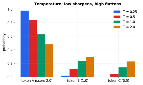
Reading it: three groups of bars, one per candidate token; within each group the bars run from low temperature (left) to high (right). For token A the bars fall as temperature rises, and for tokens B and C they rise. At T = 0.25, A takes almost everything; at T = 2 the three are much closer.
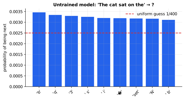
Reading it: the bars are the 12 most probable next tokens after "The cat sat on the", according to our untrained model; the dashed line is a uniform guess, 1 in 400 (0.25%). Even these favourites clear the line only modestly: the top one gets about 0.35%, 1.4 times the uniform share, and the twelfth about 1.25 times. Across all 400 tokens every probability stays between 0.74 and 1.39 times uniform, and the "favourites" are random byte fragments. That is exactly what random weights should give: a nearly flat guess with small random bumps. The machinery works, but nothing has been learned yet.
Why it matters. Use low temperature for extraction and tool calls, where you want the most likely answer, and higher temperature for creative writing. Temperature 0 reduces randomness but doesn't guarantee identical outputs on real serving hardware.
5. The loop: append and repeat
Everyday picture. Writing a sentence one word at a time, and re-reading everything you've written before choosing each new word.
Tiny worked example. A 2-token prompt, 4 new tokens. Step 1 reads 2 tokens, step 2 reads 3, step 3 reads 4, step 4 reads 5: 14 token positions to produce 4 tokens. With a 20-token prompt and 200 new tokens, the naive loop reads 23,900 positions; a KV cache reads 219.
flowchart LR
  S["ids so far"] --> M["full forward pass<br/>over ALL ids"]
  M --> P["probabilities for the next id"]
  P --> D["draw one id"]
  D --> A["append it"]
  A -->|"not done"| S
  A -->|"stop token or length limit"| OUT["decode ids to text"]
Reading it: the loop box is the whole of generation. The expensive
arrow is "full forward pass over ALL ids": every step re-reads text that
hasn't changed. Because of the causal mask, earlier tokens' internal vectors
can't change when new tokens arrive, so that repeated work is pure waste.
The KV cache (primer.ml.inference) stores it once.
The math. Total positions processed without a cache:
Level 3: the formula and its symbols
$$ W = \sum_{t=0}^{n-1} (p + t) = n\,p + \frac{n(n-1)}{2} $$
Symbols
| Symbol | Meaning here | In the example |
|---|---|---|
| $p$ | prompt length in tokens | 2 |
| $n$ | tokens to generate | 4 |
| $t$ | the step counter, from 0 to $n-1$ | 0, 1, 2, 3 |
| $p + t$ | tokens re-read at step $t$ | 2, 3, 4, 5 |
| $W$ | total positions run through the model | 14 |
In words: "each step re-reads the prompt plus everything generated so far; add that up over all steps."
With the numbers: 4 × 2 + (4 × 3) / 2 = 8 + 6 = 14, the count
generate reports as positions_processed.
Level 3: in Python
In Python:
p, n = 2, 4
# Σ over t = 0 .. n-1 of (p + t): 2 + 3 + 4 + 5
sum(p + t for t in range(n))  # → 14
# the closed form gives the same count
n * p + n * (n - 1) // 2  # → 14
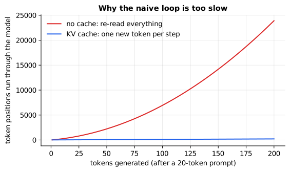
Reading it: the x-axis is how many tokens have been generated after a 20-token prompt; the y-axis is total work in token positions. The red curve bends upward: it grows with the square of the output length. The blue line (with a KV cache) grows by exactly one per token. At 200 tokens the gap is more than a hundredfold.
In code: Generation holds the generated ids, the decoded text and the positions count; naive_vs_cached_work counts the positions processed with and without a KV cache for the figure.
Why it matters. Output length drives latency and cost; this is why every serving system caches keys and values.
6. Training: the same forward pass, plus a loss
Everyday picture. A guessing game with instant feedback. Cover the next word, guess it, uncover it, and note how surprised you were. Training nudges every weight to make the surprise smaller next time.
Tiny worked example. If the model gives the right next token probability 0.5, the loss is −ln 0.5 = 0.693. Our untrained model averages 5.97 on a real sentence, close to ln 400 = 5.99, the score of a blind uniform guess.
flowchart LR
  T["training text"] --> F["forward pass<br/>(this whole lesson)"]
  F --> P["probabilities at every position"]
  P --> L["loss: −ln p(actual next token)<br/>averaged over positions"]
  L --> B["backpropagation<br/>gradient for every weight"]
  B --> U["optimizer nudges weights"]
  U -->|next batch| F
Reading it: the first two boxes are the forward pass you just traced.
Training adds the loss (how surprised the model was by the real next
tokens), then backpropagation (primer.ml.neural_net) works out how each
weight contributed, and the optimizer (primer.ml.optimizers) adjusts them.
One pass over n tokens gives n − 1 guesses at once, in parallel, which is a
big reason transformers train fast.
The math and the code. A logarithm answers "to what power must I raise e to get this number?" For probabilities between 0 and 1 it is negative, so we flip the sign; ln 1 = 0 (no surprise) and ln of a tiny number is very negative (huge surprise).
Level 3: the formula and its symbols
$$ \mathcal{L} = -\frac{1}{n-1}\sum_{i=1}^{n-1} \ln p\big(t_{i+1} \mid t_1, \ldots, t_i\big) $$
Symbols
| Symbol | Meaning here | In the example |
|---|---|---|
| $n$ | tokens in the training text | 12 ("The model reads tokens, not words.") |
| $t_i$ | the token at position $i$ | |
| $p(t_{i+1} \mid t_1,\ldots,t_i)$ | probability the model gave the actual next token, having seen everything before it; the bar $\mid$ reads "given" | ≈ 1/400 when untrained |
| $\ln$ | natural logarithm | ln(1/400) = −5.99 |
| $\frac{1}{n-1}\sum$ | the average over all $n - 1$ guesses | |
| $\mathcal{L}$ | the loss training pushes down | 5.97 |
In words: "for every position, take the log of the probability the model gave the true next token, average them, and flip the sign."
With the numbers: a uniform guess over 400 tokens gives every true token
p = 1/400, so each term is −ln(1/400) = ln 400 = 5.99. Our untrained model
scores 5.97, so it is still essentially guessing. Perplexity, e raised to
the loss, is 393: "as unsure as choosing among 393 equally likely tokens"
(next_token_loss, cross_entropy).
Level 3: in Python
In Python:
import math
# one guess that gave the true token p = 0.5
round(-math.log(0.5), 3)  # → 0.693
n = 12
# a uniform guess gives every true token 1/400
p = [1 / 400] * (n - 1)
# -(1/(n-1)) Σ ln p
L = -sum(math.log(p_i) for p_i in p) / (n - 1)
round(L, 2)  # → 5.99
Why it matters. Pretraining is exactly this, over trillions of tokens: predicting the next token well forces the model to absorb grammar, facts and reasoning patterns. Random weights produce gibberish, and training is what turns the same machinery into a useful model.
In 20 seconds
- Tokenize the prompt, look up a vector per token, add position, run the transformer blocks, score every vocabulary entry from the last position, softmax, sample, append, repeat.
- Temperature divides the scores before softmax: low is predictable, high is varied.
- The naive loop re-reads everything each step; the KV cache makes each step cost one token. Training is the same forward pass plus a next-token loss.
Self-test questions
What happens, step by step, when you send a prompt? Tokenizer turns text into ids; each id looks up an embedding; position information is added; the vectors pass through N transformer blocks; the last position's vector is scored against the whole vocabulary; softmax and sampling pick a token; it's appended and the loop repeats until a stop token.
Why does only the last position matter when generating? Its vector has attended to every earlier token and is the one trained to predict what comes next; earlier rows predict tokens we already have.
What does temperature do to the scores (2, 1, 0.5) at T = 0.5? Doubles them to (4, 2, 1) before softmax, sharpening the distribution: the top token rises from 0.63 to 0.84.
How many token positions does the naive loop process for a 2-token prompt and 4 new tokens? 2 + 3 + 4 + 5 = 14. A KV cache avoids re-reading the unchanged prefix.
What loss does an untrained model get over a 400-token vocabulary, and why? About ln 400 ≈ 5.99 (perplexity about 400), because with random, tiny weights its predictions are close to uniform.
How is training different from inference? Same forward pass, plus a loss comparing predictions to the real next tokens, then backpropagation and a weight update. Inference only runs the forward pass.
The papers behind this lesson
- Vaswani et al. (2017), Attention Is All You Need. https://arxiv.org/abs/1706.03762. The architecture inside the "transformer blocks" box. annotated companion
- Radford et al. (2019), Language Models are Unsupervised Multitask Learners (GPT-2). https://cdn.openai.com/better-language-models/language_models_are_unsupervised_multitask_learners.pdf. The decoder-only, next-token-prediction recipe this pipeline follows, including learned positions, byte-level BPE and tied embeddings.
- Brown et al. (2020), Language Models are Few-Shot Learners (GPT-3). https://arxiv.org/abs/2005.14165. Showed that scaling this same loop up produces models that follow instructions from examples in the prompt. annotated companion
- Holtzman et al. (2019), The Curious Case of Neural Text Degeneration. https://arxiv.org/abs/1904.09751. Introduced nucleus (top-p) sampling and explained why pure greedy decoding produces repetitive text.
Further reading
- Andrej Karpathy, Let's build GPT (video): https://www.youtube.com/watch?v=kCc8FmEb1nY
- Karpathy's
nanoGPT: https://github.com/karpathy/nanoGPT - Jay Alammar, The Illustrated GPT-2: https://jalammar.github.io/illustrated-gpt2/
- 3Blue1Brown, But what is a GPT? (video): https://www.youtube.com/watch?v=wjZofJX0v4M
- Hugging Face, How to generate text (decoding strategies): https://huggingface.co/blog/how-to-generate
1r""" 2# The big picture: what happens when you send a prompt 3 4Run: `python -m primer.ml.big_picture` 5 6New to the notation (vectors, sums, logarithms)? Every symbol is decoded 7where it appears, and `primer.notation` teaches them all from zero. 8 9## Level 1: The practitioner's guide 10 11**In one sentence.** A language model is a next-token scorer run in a loop: 12the prompt is cut into tokens, each token becomes a vector, the vectors 13pass through a stack of transformer blocks, the last position is scored 14against the whole vocabulary, one token is drawn, appended, and the loop 15runs again until a stop token or a length limit. 16 17**When you need it.** You need this picture whenever you set a parameter 18you can't explain (`temperature`, `top_p`, `max_tokens`), read a bill that 19counts input and output tokens differently, or debug an answer that was cut 20off, repeats itself, or comes out as gibberish. The tell: you are adjusting 21a sampling knob by trial and error, or estimating cost in words when the 22meter counts tokens. This lesson's toy tokenizer turns "Reset your password" 23into 5 tokens, and " password" is one of them while "Reset" is two, so a 24word count is only an estimate. You don't need this lesson to write a good 25prompt, and you don't need it to pick a model by its benchmark scores; you 26need it the first time a model's behaviour has to be predicted rather than 27observed. 28 29**Your options.** The loop has a few knobs a caller can turn, from the 30cheapest to the most certain: 31 32| Option | What it does | What it guarantees | What it costs | Where it lives | 33|---|---|---|---|---| 34| Leave sampling at its defaults | Draws each token in proportion to the model's probabilities (temperature 1) | The variety the model was trained to produce | Run-to-run variation | The API's defaults | 35| Lower the temperature, down to greedy | Divides the scores before softmax; at 0 it takes the single most likely token | The likely answer more often: at temperature 0.5 this lesson's top token rises from 0.63 to 0.84 | Blander text, and repetition at 0 (Holtzman et al., 2019); still not identical runs | One request parameter | 36| Cut the tail (top-k, top-p) | Keeps only the k most likely tokens, or the smallest set whose probabilities reach p | No draws from the long tail of near-zero tokens | A knob some hosted APIs have withdrawn; open-model servers keep it | One request parameter | 37| Bound the length (`max_tokens`, stop sequences) | Ends the loop at a token limit or at a string you name | A ceiling on cost and latency per call | Truncated answers if the limit is too low; check the stop reason | One request parameter | 38| Reuse the prefix (KV cache, prompt caching) | Keeps the work done on tokens that haven't changed | Each new token costs one position instead of a re-read of everything: 219 positions against 23,900 for 200 tokens after a 20-token prompt | Server memory; caching rules and prices that differ by vendor | The serving stack | 39| Constrain the output (schema, grammar) | Forbids, at every step, any token that cannot lead to a valid shape | A parseable answer by construction | A compiled schema and a small check per token | The model server (`primer.ml.structured_output`) | 40 41**How to choose.** Start from who reads the answer and how long it is. 42 43- Extraction, classification, tool calls: low temperature, a schema where 44 the server offers one, and a `max_tokens` sized to the answer. 45- Writing, brainstorming, dialogue: the default temperature, and a length 46 bound that stops runaway output rather than shaping it. 47- Long documents in the prompt: the input is read in one parallel pass, so 48 it costs money more than time; cache the unchanged prefix when you send 49 it repeatedly. 50- Agents and multi-turn systems: every turn re-sends the whole history, so 51 the prompt grows with the conversation; bound each answer and watch the 52 stop reason, because a truncated tool call is a broken one. 53- Whatever you pick, measure tokens in and out on your own traffic. Output 54 tokens are produced one loop iteration at a time, so the cheapest way to 55 make a call faster is to ask for less. 56 57**What it costs.** Two meters run. Input tokens go through the model in 58one parallel pass, so a long prompt costs money and memory more than 59time. Output tokens are produced one per trip round the loop, so latency is 60proportional to length: this lesson's naive loop reads the prompt plus 61everything generated so far at every step (14 positions to produce 4 tokens 62from a 2-token prompt), and a KV cache turns that into one position per 63token. Context is a hard ceiling: the position table has a fixed number of 64rows (64 in this toy; `max_position_embeddings` in a Hugging Face config, 65where `LlamaConfig` defaults to 2048, and 4k in the Llama 2 paper), and 66prompt plus answer must fit inside it. Quality is measured on the same loop: the training loss is 67the average of −ln p for the real next token, and perplexity is *e* raised 68to it. This lesson's untrained model scores 5.97 against 5.99 for a blind 69guess over 400 tokens (perplexity 393), and training over trillions of 70tokens (2.0T for Llama 2) is what pushes that number down. 71 72**What breaks.** 73 74- **Gibberish.** Random weights give a nearly flat guess over the 75 vocabulary, and the demo's untrained model continues "The cat" with byte 76 fragments. In practice the same symptom comes from a tokenizer that 77 doesn't match the model, so ids fetch the wrong rows of the table. Check 78 the pairing before the weights. 79- **Cut-off answers.** The loop stopped at `max_tokens`, not at a stop 80 token. Claude's API reports `end_turn` when the model finished on its own 81 and another stop reason when your limit or stop sequence ended it; treat 82 anything but a natural end as incomplete. 83- **Temperature 0 that still varies.** Greedy picks the argmax, but Claude's 84 reference says results are not fully deterministic even at 0.0, and the 85 arithmetic on real serving hardware is why. 86- **Repetition.** Always taking the most likely token produces loops of the 87 same phrase; Holtzman et al. (2019) showed it and proposed nucleus 88 sampling as the fix. 89- **A bill that surprised you.** Cost is counted in tokens, not words, and 90 a conversation re-sends its whole history every turn. 91- **A context error.** Prompt plus requested output exceeded the position 92 table. Shorten the prompt or the `max_tokens`, or retrieve less. 93 94**In the wild.** The pipeline is the decoder-only recipe of GPT-2 (Radford 95et al., 2019: byte-level BPE, learned positions, tied embeddings) that 96GPT-3 (Brown et al., 2020) scaled until instructions in the prompt were 97enough. Hugging Face's `generate()` exposes the loop's knobs in a 98`GenerationConfig` (`do_sample`, otherwise greedy; `temperature` 1.0, 99`top_k` 50, `top_p` 1.0, `max_new_tokens`, `repetition_penalty`, 100`num_beams`), and its `LlamaForCausalLM` returns logits of shape (batch, 101sequence, vocabulary) with a `logits_to_keep` option because, as its docs 102put it, only the last token's logits are needed for generation. Claude's 103Messages API offers `temperature` (0.0 to 1.0, default 1.0; models 104released after Claude Opus 4.6 accept only 1.0), `max_tokens`, 105`stop_sequences` and a `stop_reason` on every response, and lets you set 106`max_tokens` to 0 to warm the prompt cache without generating. Karpathy's 107nanoGPT is this lesson at full size, in a few hundred lines. The papers are 108linked at the end of the lesson. 109 110**Go deeper.** Level 2 traces "Reset your password" through every box with 111its shapes, works temperature by hand on three scores, counts the loop's 112positions, and measures the loss of a model that has learned nothing. If you 113only needed to set the knobs, you are done. 114 115## Level 2: How it works, from scratch 116 117This lesson wires the real pieces from the other lessons into one working 118pipeline: the tokenizer from `primer.ml.tokenization`, the transformer from 119`primer.ml.transformer`, and a sampling loop. Keep this one picture in your 120head; every other lesson zooms into one box of it. 121 122```mermaid 123flowchart LR 124 A[Prompt text] --> B[Tokenizer<br/>text to IDs] 125 B --> C[Embedding lookup<br/>IDs to vectors] 126 C --> D[Add position info] 127 D --> E[Transformer blocks<br/>repeated N times] 128 E --> F[Output layer<br/>score per vocab token] 129 F --> G[Softmax + sampling] 130 G --> H[Next token] 131 H -->|append and repeat| E 132``` 133 134**Reading it:** read left to right, then follow the loop back. The prompt is 135cut into token ids, each id picks a vector from a table, and position 136information is mixed in so order counts. The vectors pass through the 137transformer blocks, where tokens exchange information. The output layer turns 138the *last* token's final vector into a score for every token in the 139vocabulary; softmax makes those scores probabilities and one token is 140drawn. That token is appended and the loop runs again, until the model emits 141a stop token or hits a length limit. Training uses the same boxes with one 142addition, a loss, at the end (section 6). 143 144## 1. Text to ids: the coat check 145 146**Everyday picture.** A coat check. You hand over a coat (a piece of text) 147and get back a numbered ticket (a token id). The model only ever handles the 148tickets. 149 150**Tiny worked example.** With this module's toy tokenizer, "Reset your 151password" becomes 5 tickets: `Re` `set` ` y` `our` ` password` → 152**[346, 377, 309, 328, 291]**. The common word " password" got a single 153ticket; the rarer pieces got several. 154 155```mermaid 156flowchart LR 157 T["'Reset your password'"] --> TK["tokenizer<br/>(learned kit of 400 pieces)"] 158 TK --> I["[346, 377, 309, 328, 291]"] 159``` 160 161**Reading it:** one box, text in and integers out. Everything to the right 162of this box works only with integers and vectors. 163 164**The code.** `tok.encode(prompt)`; how the kit is learned is the whole of 165`primer.ml.tokenization`. 166 167**In code:** `build_pipeline` trains the toy tokenizer (`primer.ml.tokenization.ByteBPE`) and builds an untrained `primer.ml.transformer.TinyGPT` sized to its vocabulary. 168 169**Why it matters.** Prompt length, price and context limits are all counted 170in these tickets. 171 172## 2. Ids to vectors: a lookup, not a computation 173 174**Everyday picture.** A dictionary where ticket number 291 opens to page 291, 175and each page holds a list of numbers describing that token. A second 176dictionary, indexed by seat number, describes *where* the token sits. 177 178**Tiny worked example.** The table has 400 rows (one per token) of 32 179numbers. Id 291 fetches row 291. The 5 ids fetch 5 rows: a 5 × 32 grid. Row 180i of the position table (i = 0 to 4) is added to row i of that grid. 181 182```mermaid 183flowchart LR 184 I["ids (5)"] --> E["token table<br/>400 × 32"] 185 E --> X["5 × 32: what each token is"] 186 P["positions 0..4"] --> PT["position table<br/>64 × 32"] 187 PT --> Y["5 × 32: where each token is"] 188 X --> ADD(("+")) 189 Y --> ADD 190 ADD --> OUT["5 × 32 input to the blocks"] 191``` 192 193**Reading it:** two lookups, one add. Nothing is multiplied here, rows are 194simply fetched, which is why this step is nearly free. The tables themselves 195are learned during training, so similar tokens end up with similar rows (see 196`primer.ml.embeddings`). 197 198**The math and the code.** 199 200$$ 201x_i = E_{t_i} + P_i 202$$ 203 204**Symbols** 205 206| Symbol | Meaning here | In the example | 207|---|---|---| 208| $i$ | a token's position in the prompt, from 0 | 4 (the last token) | 209| $t_i$ | the token id at position $i$ | $t_4$ = 291 | 210| $E$ | the token embedding table | 400 × 32 | 211| $E_{t_i}$ | row $t_i$ of that table | row 291: 32 numbers | 212| $P_i$ | row $i$ of the position table | row 4: 32 numbers | 213| $x_i$ | what the first block receives for position $i$ | 32 numbers | 214 215**In words:** "each token's input vector is its token's row plus its 216position's row." 217 218**With the numbers:** $x_4 = E_{291} + P_4$, one 32-number list plus 219another. The code is `model.wte[ids] + model.wpe[:len(ids)]`. In miniature, 220with 3-number rows instead of 32: $E_{291}$ = (0.2, −0.1, 0.5) and $P_4$ = 221(0.1, 0.3, −0.2) give $x_4$ = (0.3, 0.2, 0.3). 222 223**In Python:** 224 225```python 226# row 291 of the token table (3 numbers, not 32) 227E_291 = [0.2, -0.1, 0.5] 228# row 4 of the position table 229P_4 = [0.1, 0.3, -0.2] 230# E_(t_i) + P_i, number by number 231x_4 = [round(e + p, 2) for e, p in zip(E_291, P_4)] 232x_4 # → [0.3, 0.2, 0.3] 233``` 234 235**In code:** `trace` does both lookups and the add, and keeps every stage's result so you can inspect the grid before and after positions are mixed in. 236 237**Why it matters.** This is the only place a token's identity enters the 238model; every later step works on these vectors. 239 240## 3. The transformer blocks: rounds of meeting and desk work 241 242**Everyday picture.** The team from `primer.ml.transformer`: each round is a 243meeting where every token listens to the others (attention), then desk work 244where each token thinks alone (feed-forward). This toy runs 2 rounds; large 245models run dozens. 246 247**Tiny worked example.** The 5 × 32 grid goes into block 1 and comes out 2485 × 32; the same through block 2. By the end, the vector at the last position 249("password") has absorbed information from "Re", "set", "y" and "our". 250 251```mermaid 252flowchart LR 253 X["5 × 32"] --> B1["block 1<br/>meeting + desk work"] --> B2["block 2"] --> LN["final norm"] --> H["5 × 32<br/>context-aware vectors"] 254``` 255 256**Reading it:** the shape never changes, only the contents. Each block 257edits every token's vector by adding what it learned from the others. 258 259**The math and the code.** 260 261$$ 262h = \text{LN}\big(\text{Block}_N(\cdots\text{Block}_2(\text{Block}_1(x))\cdots)\big) 263$$ 264 265**Symbols** 266 267| Symbol | Meaning here | In the example | 268|---|---|---| 269| $x$ | the 5 × 32 input grid from section 2 | | 270| $\text{Block}_k$ | the $k$-th transformer block | $N$ = 2 | 271| $\cdots$ | "and so on, for every block in between" | | 272| $\text{LN}$ | the final layer norm | | 273| $h$ | the context-aware vectors | 5 × 32 | 274 275**In words:** "run the input through every block in turn, then normalize." 276 277**With the numbers:** here N = 2, so h = LN(Block₂(Block₁(x))). The code is 278the `for block in model.blocks` loop in `trace`. In miniature, with one 2793-number vector and two stand-in blocks that each add an edit: x = (1, 2, 3), 280Block₁ adds (0, 1, 0) and Block₂ adds (0, 0, 2), giving (1, 3, 5). The final 281norm subtracts the mean (3) and divides by the spread (1.63), so 282h = (−1.22, 0, 1.22). 283 284**In Python:** 285 286```python 287import statistics 288x = [1.0, 2.0, 3.0] 289# a stand-in edit 290def block_1(v): return [v_i + d for v_i, d in zip(v, [0, 1, 0])] 291def block_2(v): return [v_i + d for v_i, d in zip(v, [0, 0, 2])] 292def LN(v): 293 mu, sigma = statistics.fmean(v), statistics.pstdev(v) 294 # centre, then rescale 295 return [round((v_i - mu) / sigma, 2) for v_i in v] 296h = x 297# Block_1 first, then Block_2 ... up to Block_N 298for block in [block_1, block_2]: 299 h = block(h) 300h # → [1.0, 3.0, 5.0] 301LN(h) # → [-1.22, 0.0, 1.22] 302``` 303 304**Why it matters.** This is where nearly all the compute and all the 305"understanding" happen. 306 307## 4. Scores, softmax and temperature 308 309**Everyday picture.** A scoreboard with one line for every token in the 310vocabulary. Softmax turns the scores into shares of a pie. **Temperature** 311sets how adventurous the pick is: low temperature almost always takes the 312biggest slice; high temperature gives the small slices a real chance. 313 314**Tiny worked example.** Three candidate tokens scored 2.0, 1.0 and 0.5. 315 316| temperature | p(A) | p(B) | p(C) | 317|---|---|---|---| 318| 0 (greedy) | 1.000 | 0.000 | 0.000 | 319| 0.5 | 0.844 | 0.114 | 0.042 | 320| 1 | 0.629 | 0.231 | 0.140 | 321| 2 | 0.481 | 0.292 | 0.227 | 322 323```mermaid 324flowchart LR 325 H["last row of h<br/>32 numbers"] --> S["× token tableᵀ<br/>400 scores"] 326 S --> T["÷ temperature"] 327 T --> SM["softmax<br/>400 probabilities"] 328 SM --> PICK["draw one token"] 329``` 330 331**Reading it:** only the last position's vector is used to choose the next 332token. It is scored against every token's embedding, the scores are divided 333by the temperature, softmax turns them into probabilities that sum to 1, and 334one token is drawn at random in proportion to them. 335 336**The math and the code.** **Softmax** raises *e* (≈ 2.718) to the power of 337each score, so bigger scores get disproportionately bigger shares, then 338divides by the total so the shares add up to 1: 339 340$$ 341p_i = \frac{e^{z_i / T}}{\sum_{j=1}^{V} e^{z_j / T}} 342$$ 343 344**Symbols** 345 346| Symbol | Meaning here | In the example | 347|---|---|---| 348| $z_i$ | the score of candidate token $i$ | $z_A$ = 2.0 | 349| $T$ | the temperature | 0.5 | 350| $e^{\cdot}$ | *e* ≈ 2.718 raised to that power | $e^{4}$ = 54.6 | 351| $V$ | number of candidates (the vocabulary size) | 3 here, 400 in the model | 352| $\sum_{j=1}^{V}$ | add up over every candidate $j$ | | 353| $p_i$ | probability that token $i$ comes next | 0.844 | 354 355**In words:** "the chance of token *i* is *e* to the power of its score over 356the temperature, divided by the same quantity summed over all tokens." 357 358**With the numbers:** T = 0.5 doubles every score to (4, 2, 1): e⁴ = 54.6, 359e² = 7.39, e¹ = 2.72, total 64.7, so p(A) = 54.6 / 64.7 = **0.844** 360(`next_token_probs`). Temperature 0 is the limit case: all probability on the 361top score. 362 363**In Python:** 364 365```python 366import math 367z = [2.0, 1.0, 0.5] 368T = 0.5 369# e^(z_i / T) for each candidate 370exps = [math.exp(z_i / T) for z_i in z] 371[round(e, 2) for e in exps] # → [54.6, 7.39, 2.72] 372# Σ_j e^(z_j / T) 373total = sum(exps) 374round(total, 1) # → 64.7 375# p_i: each share of the total 376[round(e / total, 3) for e in exps] # → [0.844, 0.114, 0.042] 377``` 378 379 380 381**Reading it:** three groups of bars, one per candidate token; within each 382group the bars run from low temperature (left) to high (right). For token A 383the bars fall as temperature rises, and for tokens B and C they rise. At 384T = 0.25, A takes almost everything; at T = 2 the three are much closer. 385 386 387 388**Reading it:** the bars are the 12 most probable next tokens after "The cat 389sat on the", according to our untrained model; the dashed line is a uniform 390guess, 1 in 400 (0.25%). Even these favourites clear the line only 391modestly: the top one gets about 0.35%, 1.4 times the uniform share, and the 392twelfth about 1.25 times. Across all 400 tokens every probability stays 393between 0.74 and 1.39 times uniform, and the "favourites" are random byte 394fragments. That is exactly what random weights should give: a nearly flat 395guess with small random bumps. The machinery works, but nothing has been 396learned yet. 397 398**Why it matters.** Use low temperature for extraction and tool calls, 399where you want the most likely answer, and higher temperature for creative 400writing. Temperature 0 reduces randomness but doesn't guarantee identical 401outputs on real serving hardware. 402 403## 5. The loop: append and repeat 404 405**Everyday picture.** Writing a sentence one word at a time, and re-reading 406everything you've written before choosing each new word. 407 408**Tiny worked example.** A 2-token prompt, 4 new tokens. Step 1 reads 2 409tokens, step 2 reads 3, step 3 reads 4, step 4 reads 5: **14** token 410positions to produce 4 tokens. With a 20-token prompt and 200 new tokens, the 411naive loop reads 23,900 positions; a KV cache reads 219. 412 413```mermaid 414flowchart LR 415 S["ids so far"] --> M["full forward pass<br/>over ALL ids"] 416 M --> P["probabilities for the next id"] 417 P --> D["draw one id"] 418 D --> A["append it"] 419 A -->|"not done"| S 420 A -->|"stop token or length limit"| OUT["decode ids to text"] 421``` 422 423**Reading it:** the loop box is the whole of generation. The expensive 424arrow is "full forward pass over ALL ids": every step re-reads text that 425hasn't changed. Because of the causal mask, earlier tokens' internal vectors 426can't change when new tokens arrive, so that repeated work is pure waste. 427The KV cache (`primer.ml.inference`) stores it once. 428 429**The math.** Total positions processed without a cache: 430 431$$ 432W = \sum_{t=0}^{n-1} (p + t) = n\,p + \frac{n(n-1)}{2} 433$$ 434 435**Symbols** 436 437| Symbol | Meaning here | In the example | 438|---|---|---| 439| $p$ | prompt length in tokens | 2 | 440| $n$ | tokens to generate | 4 | 441| $t$ | the step counter, from 0 to $n-1$ | 0, 1, 2, 3 | 442| $p + t$ | tokens re-read at step $t$ | 2, 3, 4, 5 | 443| $W$ | total positions run through the model | 14 | 444 445**In words:** "each step re-reads the prompt plus everything generated so 446far; add that up over all steps." 447 448**With the numbers:** 4 × 2 + (4 × 3) / 2 = 8 + 6 = **14**, the count 449`generate` reports as `positions_processed`. 450 451**In Python:** 452 453```python 454p, n = 2, 4 455# Σ over t = 0 .. n-1 of (p + t): 2 + 3 + 4 + 5 456sum(p + t for t in range(n)) # → 14 457# the closed form gives the same count 458n * p + n * (n - 1) // 2 # → 14 459``` 460 461 462 463**Reading it:** the x-axis is how many tokens have been generated after a 46420-token prompt; the y-axis is total work in token positions. The red curve 465bends upward: it grows with the square of the output length. The blue line 466(with a KV cache) grows by exactly one per token. At 200 tokens the gap is 467more than a hundredfold. 468 469**In code:** `Generation` holds the generated ids, the decoded text and the positions count; `naive_vs_cached_work` counts the positions processed with and without a KV cache for the figure. 470 471**Why it matters.** Output length drives latency and cost; this is why 472every serving system caches keys and values. 473 474## 6. Training: the same forward pass, plus a loss 475 476**Everyday picture.** A guessing game with instant feedback. Cover the next 477word, guess it, uncover it, and note how surprised you were. Training nudges 478every weight to make the surprise smaller next time. 479 480**Tiny worked example.** If the model gives the right next token probability 4810.5, the loss is −ln 0.5 = **0.693**. Our untrained model averages **5.97** on 482a real sentence, close to ln 400 = 5.99, the score of a blind uniform guess. 483 484```mermaid 485flowchart LR 486 T["training text"] --> F["forward pass<br/>(this whole lesson)"] 487 F --> P["probabilities at every position"] 488 P --> L["loss: −ln p(actual next token)<br/>averaged over positions"] 489 L --> B["backpropagation<br/>gradient for every weight"] 490 B --> U["optimizer nudges weights"] 491 U -->|next batch| F 492``` 493 494**Reading it:** the first two boxes are the forward pass you just traced. 495Training adds the loss (how surprised the model was by the real next 496tokens), then backpropagation (`primer.ml.neural_net`) works out how each 497weight contributed, and the optimizer (`primer.ml.optimizers`) adjusts them. 498One pass over n tokens gives n − 1 guesses at once, in parallel, which is a 499big reason transformers train fast. 500 501**The math and the code.** A **logarithm** answers "to what power must I 502raise *e* to get this number?" For probabilities between 0 and 1 it is 503negative, so we flip the sign; ln 1 = 0 (no surprise) and ln of a tiny 504number is very negative (huge surprise). 505 506$$ 507\mathcal{L} = -\frac{1}{n-1}\sum_{i=1}^{n-1} \ln p\big(t_{i+1} \mid t_1, \ldots, t_i\big) 508$$ 509 510**Symbols** 511 512| Symbol | Meaning here | In the example | 513|---|---|---| 514| $n$ | tokens in the training text | 12 ("The model reads tokens, not words.") | 515| $t_i$ | the token at position $i$ | | 516| $p(t_{i+1} \mid t_1,\ldots,t_i)$ | probability the model gave the *actual* next token, having seen everything before it; the bar $\mid$ reads "given" | ≈ 1/400 when untrained | 517| $\ln$ | natural logarithm | ln(1/400) = −5.99 | 518| $\frac{1}{n-1}\sum$ | the average over all $n - 1$ guesses | | 519| $\mathcal{L}$ | the loss training pushes down | 5.97 | 520 521**In words:** "for every position, take the log of the probability the model 522gave the true next token, average them, and flip the sign." 523 524**With the numbers:** a uniform guess over 400 tokens gives every true token 525p = 1/400, so each term is −ln(1/400) = ln 400 = **5.99**. Our untrained model 526scores 5.97, so it is still essentially guessing. **Perplexity**, e raised to 527the loss, is 393: "as unsure as choosing among 393 equally likely tokens" 528(`next_token_loss`, `cross_entropy`). 529 530**In Python:** 531 532```python 533import math 534# one guess that gave the true token p = 0.5 535round(-math.log(0.5), 3) # → 0.693 536n = 12 537# a uniform guess gives every true token 1/400 538p = [1 / 400] * (n - 1) 539# -(1/(n-1)) Σ ln p 540L = -sum(math.log(p_i) for p_i in p) / (n - 1) 541round(L, 2) # → 5.99 542``` 543 544**Why it matters.** Pretraining is exactly this, over trillions of tokens: 545predicting the next token well forces the model to absorb grammar, facts and 546reasoning patterns. Random weights produce gibberish, and training is what 547turns the same machinery into a useful model. 548 549## In 20 seconds 550- Tokenize the prompt, look up a vector per token, add position, run the 551 transformer blocks, score every vocabulary entry from the last position, 552 softmax, sample, append, repeat. 553- Temperature divides the scores before softmax: low is predictable, high is 554 varied. 555- The naive loop re-reads everything each step; the KV cache makes each step 556 cost one token. Training is the same forward pass plus a next-token loss. 557 558## Self-test questions 559 560**What happens, step by step, when you send a prompt?** 561Tokenizer turns text into ids; each id looks up an embedding; position 562information is added; the vectors pass through N transformer blocks; the last 563position's vector is scored against the whole vocabulary; softmax and sampling 564pick a token; it's appended and the loop repeats until a stop token. 565 566**Why does only the last position matter when generating?** 567Its vector has attended to every earlier token and is the one trained to 568predict what comes next; earlier rows predict tokens we already have. 569 570**What does temperature do to the scores (2, 1, 0.5) at T = 0.5?** 571Doubles them to (4, 2, 1) before softmax, sharpening the distribution: the 572top token rises from 0.63 to 0.84. 573 574**How many token positions does the naive loop process for a 2-token prompt and 4 new tokens?** 5752 + 3 + 4 + 5 = 14. A KV cache avoids re-reading the unchanged prefix. 576 577**What loss does an untrained model get over a 400-token vocabulary, and why?** 578About ln 400 ≈ 5.99 (perplexity about 400), because with random, tiny weights 579its predictions are close to uniform. 580 581**How is training different from inference?** 582Same forward pass, plus a loss comparing predictions to the real next tokens, 583then backpropagation and a weight update. Inference only runs the forward pass. 584 585## The papers behind this lesson 586 587- **Vaswani et al. (2017), *Attention Is All You Need*.** https://arxiv.org/abs/1706.03762. 588 The architecture inside the "transformer blocks" box. 589 [annotated companion](../../papers/attention-is-all-you-need.html) 590- **Radford et al. (2019), *Language Models are Unsupervised Multitask Learners* (GPT-2).** 591 https://cdn.openai.com/better-language-models/language_models_are_unsupervised_multitask_learners.pdf. 592 The decoder-only, next-token-prediction recipe this pipeline follows, 593 including learned positions, byte-level BPE and tied embeddings. 594- **Brown et al. (2020), *Language Models are Few-Shot Learners* (GPT-3).** 595 https://arxiv.org/abs/2005.14165. Showed that scaling this same loop up 596 produces models that follow instructions from examples in the prompt. 597 [annotated companion](../../papers/gpt-3.html) 598- **Holtzman et al. (2019), *The Curious Case of Neural Text Degeneration*.** 599 https://arxiv.org/abs/1904.09751. Introduced nucleus (top-p) sampling and 600 explained why pure greedy decoding produces repetitive text. 601 602## Further reading 603- Andrej Karpathy, *Let's build GPT* (video): https://www.youtube.com/watch?v=kCc8FmEb1nY 604- Karpathy's `nanoGPT`: https://github.com/karpathy/nanoGPT 605- Jay Alammar, *The Illustrated GPT-2*: https://jalammar.github.io/illustrated-gpt2/ 606- 3Blue1Brown, *But what is a GPT?* (video): https://www.youtube.com/watch?v=wjZofJX0v4M 607- Hugging Face, *How to generate text* (decoding strategies): https://huggingface.co/blog/how-to-generate 608""" 609 610from __future__ import annotations 611 612from dataclasses import dataclass 613 614import numpy as np 615 616from primer._show import banner, say, table, takeaway 617from primer.ml.tokenization import ByteBPE, trained_tokenizer 618from primer.ml.transformer import TinyGPT, layer_norm 619 620# Model size for the walkthrough: small enough to run instantly in NumPy. 621D_MODEL, N_LAYERS, N_HEADS, MAX_LEN = 32, 2, 4, 64 622 623 624def build_pipeline(seed: int = 0) -> tuple[ByteBPE, TinyGPT]: 625 """A trained toy tokenizer plus an *untrained* TinyGPT sized to its vocabulary.""" 626 tok = trained_tokenizer() 627 model = TinyGPT(tok.vocab_size, D_MODEL, N_LAYERS, N_HEADS, MAX_LEN, seed=seed) 628 return tok, model 629 630 631# --------------------------------------------------------------------------- 632# 1. One forward pass, stage by stage 633# --------------------------------------------------------------------------- 634 635 636def next_token_probs(logits: np.ndarray, temperature: float = 1.0) -> np.ndarray: 637 """Turn one row of scores into next-token probabilities. 638 639 Temperature divides the scores before softmax: below 1 sharpens the 640 distribution (more predictable), above 1 flattens it (more varied). 641 Temperature 0 is the limit: all probability on the top score (greedy). 642 """ 643 if temperature == 0: 644 p = np.zeros_like(logits, dtype=float) 645 p[np.argmax(logits)] = 1.0 646 return p 647 z = logits / temperature 648 e = np.exp(z - z.max()) # subtract the max so exp never overflows 649 return e / e.sum() 650 651 652def trace(prompt: str, tok: ByteBPE, model: TinyGPT) -> dict[str, np.ndarray]: 653 """Run one prompt through every stage and keep each intermediate result.""" 654 ids = np.array(tok.encode(prompt)) # (n,) text -> integers 655 emb = model.wte[ids] # (n, d) integers -> vectors (a table lookup) 656 x = emb + model.wpe[: len(ids)] # (n, d) add "where" to "what" 657 for block in model.blocks: # (n, d) N rounds of meeting + desk work 658 x = block(x) 659 h = layer_norm(x, model.lnf_g, model.lnf_b) 660 logits = h @ model.wte.T # (n, vocab) a score for every possible next token 661 return { 662 "ids": ids, 663 "embeddings": emb, 664 "with_positions": emb + model.wpe[: len(ids)], 665 "after_blocks": x, 666 "logits": logits, 667 "next_token_probs": next_token_probs(logits[-1]), # only the last row predicts what comes next 668 } 669 670 671# --------------------------------------------------------------------------- 672# 2. The generation loop: predict, sample, append, repeat 673# --------------------------------------------------------------------------- 674 675 676@dataclass 677class Generation: 678 ids: list[int] 679 text: str 680 positions_processed: int # total token positions run through the model 681 682 683def generate( 684 prompt: str, n_new: int, tok: ByteBPE, model: TinyGPT, temperature: float = 1.0, seed: int = 0 685) -> Generation: 686 """The naive autoregressive loop: re-run the whole sequence for every new token. 687 688 Step t processes all (prompt + t) tokens again, so total work grows with 689 the square of the output length. The KV cache (primer.ml.inference) 690 stores each token's keys and values so every step only processes the one 691 new token. A real model also stops at an end-of-text token; this toy just 692 stops after n_new. 693 """ 694 rng = np.random.default_rng(seed) 695 ids = tok.encode(prompt) 696 processed = 0 697 for _ in range(n_new): 698 logits = model(np.array(ids)) 699 processed += len(ids) 700 p = next_token_probs(logits[-1], temperature) 701 ids.append(int(rng.choice(len(p), p=p))) 702 return Generation(ids=ids, text=tok.decode(ids), positions_processed=processed) 703 704 705# --------------------------------------------------------------------------- 706# 3. Training: the same forward pass, plus a loss 707# --------------------------------------------------------------------------- 708 709 710def cross_entropy(probs: np.ndarray, target: int) -> float: 711 """−ln(probability given to the right answer). Big when confidently wrong.""" 712 return float(-np.log(probs[target])) 713 714 715def next_token_loss(text: str, tok: ByteBPE, model: TinyGPT) -> float: 716 """Average next-token cross-entropy over `text`, the number training pushes down. 717 718 Every position predicts the token after it, so one forward pass over n 719 tokens gives n-1 training examples at once, in parallel. That is a big 720 reason transformers train so much faster than RNNs. 721 """ 722 ids = tok.encode(text) 723 logits = model(np.array(ids)) 724 losses = [cross_entropy(next_token_probs(logits[i]), ids[i + 1]) for i in range(len(ids) - 1)] 725 return float(np.mean(losses)) 726 727 728# --------------------------------------------------------------------------- 729# 4. Figures (rendered to docs/figures by `make figures`) 730# --------------------------------------------------------------------------- 731 732TEMPERATURE_SCORES = np.array([2.0, 1.0, 0.5]) 733 734 735def naive_vs_cached_work(prompt_len: int, max_new: int) -> list[tuple[int, int, int]]: 736 """(new tokens, positions processed without a cache, with a KV cache). 737 738 Without a cache step t re-runs prompt_len + t positions. With a cache the 739 first step runs the prompt once (prefill), and every later step runs just 740 the one new token. 741 """ 742 rows = [] 743 for n in range(1, max_new + 1): 744 naive = sum(prompt_len + t for t in range(n)) 745 cached = prompt_len + (n - 1) 746 rows.append((n, naive, cached)) 747 return rows 748 749 750def figures() -> dict: 751 """Plot this lesson's data. matplotlib is imported here, and only here.""" 752 import matplotlib 753 754 matplotlib.use("Agg") 755 import matplotlib.pyplot as plt 756 757 BLUE, RED, MUTED = "#2563eb", "#dc2626", "#9ca3af" 758 figs = {} 759 tok, model = build_pipeline() 760 761 p = trace("The cat sat on the", tok, model)["next_token_probs"] 762 top = np.argsort(-p)[:12] 763 fig, ax = plt.subplots(figsize=(6.5, 3.6)) 764 ax.bar([repr(tok.decode([int(i)])) for i in top], p[top], color=BLUE) 765 ax.axhline(1 / len(p), color=RED, ls="--", label=f"uniform guess 1/{len(p)}") 766 ax.set_ylabel("probability of being next") 767 ax.set_title("Untrained model: 'The cat sat on the' → ?") 768 ax.tick_params(axis="x", rotation=45) 769 ax.legend(frameon=False) 770 fig.tight_layout() 771 figs["untrained_next_token"] = fig 772 773 temps = (0.25, 0.5, 1.0, 2.0) 774 fig, ax = plt.subplots(figsize=(6, 3.6)) 775 width = 0.2 776 for j, T in enumerate(temps): 777 ax.bar(np.arange(3) + (j - 1.5) * width, next_token_probs(TEMPERATURE_SCORES, T), width, label=f"T = {T}") 778 ax.set_xticks(range(3), ["token A (score 2.0)", "token B (1.0)", "token C (0.5)"]) 779 ax.set_ylabel("probability") 780 ax.set_title("Temperature: low sharpens, high flattens") 781 ax.legend(frameon=False) 782 fig.tight_layout() 783 figs["temperature"] = fig 784 785 rows = naive_vs_cached_work(prompt_len=20, max_new=200) 786 fig, ax = plt.subplots(figsize=(6, 3.6)) 787 ax.plot([r[0] for r in rows], [r[1] for r in rows], color=RED, label="no cache: re-read everything") 788 ax.plot([r[0] for r in rows], [r[2] for r in rows], color=BLUE, label="KV cache: one new token per step") 789 ax.set_xlabel("tokens generated (after a 20-token prompt)") 790 ax.set_ylabel("token positions run through the model") 791 ax.set_title("Why the naive loop is too slow") 792 ax.legend(frameon=False) 793 fig.tight_layout() 794 figs["loop_cost"] = fig 795 return figs 796 797 798# --------------------------------------------------------------------------- 799# 5. Narrated walkthrough 800# --------------------------------------------------------------------------- 801 802 803def demo() -> None: 804 tok, model = build_pipeline() 805 prompt = "Reset your password" 806 807 banner("1. Text -> ids -> vectors -> blocks -> scores") 808 st = trace(prompt, tok, model) 809 table( 810 ["stage", "shape", "what it holds"], 811 [ 812 ("ids", st["ids"].shape, f"{st['ids'].tolist()} = {tok.tokens(prompt)}"), 813 ("embeddings", st["embeddings"].shape, "one row of the token table per id"), 814 ("with positions", st["with_positions"].shape, "plus one row of the position table"), 815 ("after blocks", st["after_blocks"].shape, f"{N_LAYERS} rounds of attention + feed-forward"), 816 ("logits", st["logits"].shape, f"a score for all {tok.vocab_size} tokens, per position"), 817 ("next-token probs", st["next_token_probs"].shape, "softmax of the LAST row only"), 818 ], 819 ) 820 takeaway("Only the last position's scores decide the next token; the rest matter during training.") 821 822 banner("2. Temperature on the scores (2.0, 1.0, 0.5)") 823 table( 824 ["temperature", "p(A)", "p(B)", "p(C)"], 825 [(T, *next_token_probs(TEMPERATURE_SCORES, T)) for T in (0.0, 0.5, 1.0, 2.0)], 826 floatfmt=".3f", 827 ) 828 829 banner("3. The loop: predict, sample, append, repeat") 830 g = generate("The cat", 12, tok, model, seed=0) 831 say( 832 f""" 833 Continuation of 'The cat': {g.text!r}. It's gibberish, and it should be: 834 the weights are random, so every next token is close to a uniform guess 835 over {tok.vocab_size} tokens. The machinery is identical to a real model's; 836 only the numbers inside the matrices are missing. They come from training. 837 This loop ran {g.positions_processed} token positions to produce 12 tokens, 838 because it re-reads the whole sequence every step (see primer.ml.inference 839 for the KV cache). 840 """ 841 ) 842 843 banner("4. Training = the same forward pass + a loss") 844 loss = next_token_loss("The model reads tokens, not words.", tok, model) 845 say( 846 f""" 847 Average next-token loss of the untrained model: {loss:.2f}. A uniform guess 848 over {tok.vocab_size} tokens scores ln {tok.vocab_size} = {np.log(tok.vocab_size):.2f}. 849 Perplexity e^loss = {np.exp(loss):.0f}: the model is as unsure as picking among 850 ~{np.exp(loss):.0f} equally likely tokens. Training nudges every weight to push 851 this number down, across trillions of tokens. 852 """ 853 ) 854 takeaway("A language model is a next-token scorer run in a loop; training makes its scores good.") 855 856 857if __name__ == "__main__": 858 demo()
625def build_pipeline(seed: int = 0) -> tuple[ByteBPE, TinyGPT]:
626    """A trained toy tokenizer plus an *untrained* TinyGPT sized to its vocabulary."""
627    tok = trained_tokenizer()
628    model = TinyGPT(tok.vocab_size, D_MODEL, N_LAYERS, N_HEADS, MAX_LEN, seed=seed)
629    return tok, model
A trained toy tokenizer plus an untrained TinyGPT sized to its vocabulary.
637def next_token_probs(logits: np.ndarray, temperature: float = 1.0) -> np.ndarray:
638    """Turn one row of scores into next-token probabilities.
639
640    Temperature divides the scores before softmax: below 1 sharpens the
641    distribution (more predictable), above 1 flattens it (more varied).
642    Temperature 0 is the limit: all probability on the top score (greedy).
643    """
644    if temperature == 0:
645        p = np.zeros_like(logits, dtype=float)
646        p[np.argmax(logits)] = 1.0
647        return p
648    z = logits / temperature
649    e = np.exp(z - z.max())  # subtract the max so exp never overflows
650    return e / e.sum()
Turn one row of scores into next-token probabilities.
Temperature divides the scores before softmax: below 1 sharpens the distribution (more predictable), above 1 flattens it (more varied). Temperature 0 is the limit: all probability on the top score (greedy).
653def trace(prompt: str, tok: ByteBPE, model: TinyGPT) -> dict[str, np.ndarray]:
654    """Run one prompt through every stage and keep each intermediate result."""
655    ids = np.array(tok.encode(prompt))  # (n,)       text -> integers
656    emb = model.wte[ids]  # (n, d)     integers -> vectors (a table lookup)
657    x = emb + model.wpe[: len(ids)]  # (n, d)     add "where" to "what"
658    for block in model.blocks:  # (n, d)     N rounds of meeting + desk work
659        x = block(x)
660    h = layer_norm(x, model.lnf_g, model.lnf_b)
661    logits = h @ model.wte.T  # (n, vocab) a score for every possible next token
662    return {
663        "ids": ids,
664        "embeddings": emb,
665        "with_positions": emb + model.wpe[: len(ids)],
666        "after_blocks": x,
667        "logits": logits,
668        "next_token_probs": next_token_probs(logits[-1]),  # only the last row predicts what comes next
669    }
Run one prompt through every stage and keep each intermediate result.
677@dataclass
678class Generation:
679    ids: list[int]
680    text: str
681    positions_processed: int  # total token positions run through the model
684def generate(
685    prompt: str, n_new: int, tok: ByteBPE, model: TinyGPT, temperature: float = 1.0, seed: int = 0
686) -> Generation:
687    """The naive autoregressive loop: re-run the whole sequence for every new token.
688
689    Step t processes all (prompt + t) tokens again, so total work grows with
690    the square of the output length. The KV cache (primer.ml.inference)
691    stores each token's keys and values so every step only processes the one
692    new token. A real model also stops at an end-of-text token; this toy just
693    stops after n_new.
694    """
695    rng = np.random.default_rng(seed)
696    ids = tok.encode(prompt)
697    processed = 0
698    for _ in range(n_new):
699        logits = model(np.array(ids))
700        processed += len(ids)
701        p = next_token_probs(logits[-1], temperature)
702        ids.append(int(rng.choice(len(p), p=p)))
703    return Generation(ids=ids, text=tok.decode(ids), positions_processed=processed)
The naive autoregressive loop: re-run the whole sequence for every new token.
Step t processes all (prompt + t) tokens again, so total work grows with the square of the output length. The KV cache (primer.ml.inference) stores each token's keys and values so every step only processes the one new token. A real model also stops at an end-of-text token; this toy just stops after n_new.
711def cross_entropy(probs: np.ndarray, target: int) -> float:
712    """−ln(probability given to the right answer). Big when confidently wrong."""
713    return float(-np.log(probs[target]))
−ln(probability given to the right answer). Big when confidently wrong.
716def next_token_loss(text: str, tok: ByteBPE, model: TinyGPT) -> float:
717    """Average next-token cross-entropy over `text`, the number training pushes down.
718
719    Every position predicts the token after it, so one forward pass over n
720    tokens gives n-1 training examples at once, in parallel. That is a big
721    reason transformers train so much faster than RNNs.
722    """
723    ids = tok.encode(text)
724    logits = model(np.array(ids))
725    losses = [cross_entropy(next_token_probs(logits[i]), ids[i + 1]) for i in range(len(ids) - 1)]
726    return float(np.mean(losses))
Average next-token cross-entropy over text, the number training pushes down.
Every position predicts the token after it, so one forward pass over n tokens gives n-1 training examples at once, in parallel. That is a big reason transformers train so much faster than RNNs.
736def naive_vs_cached_work(prompt_len: int, max_new: int) -> list[tuple[int, int, int]]:
737    """(new tokens, positions processed without a cache, with a KV cache).
738
739    Without a cache step t re-runs prompt_len + t positions. With a cache the
740    first step runs the prompt once (prefill), and every later step runs just
741    the one new token.
742    """
743    rows = []
744    for n in range(1, max_new + 1):
745        naive = sum(prompt_len + t for t in range(n))
746        cached = prompt_len + (n - 1)
747        rows.append((n, naive, cached))
748    return rows
(new tokens, positions processed without a cache, with a KV cache).
Without a cache step t re-runs prompt_len + t positions. With a cache the first step runs the prompt once (prefill), and every later step runs just the one new token.
751def figures() -> dict:
752    """Plot this lesson's data. matplotlib is imported here, and only here."""
753    import matplotlib
754
755    matplotlib.use("Agg")
756    import matplotlib.pyplot as plt
757
758    BLUE, RED, MUTED = "#2563eb", "#dc2626", "#9ca3af"
759    figs = {}
760    tok, model = build_pipeline()
761
762    p = trace("The cat sat on the", tok, model)["next_token_probs"]
763    top = np.argsort(-p)[:12]
764    fig, ax = plt.subplots(figsize=(6.5, 3.6))
765    ax.bar([repr(tok.decode([int(i)])) for i in top], p[top], color=BLUE)
766    ax.axhline(1 / len(p), color=RED, ls="--", label=f"uniform guess 1/{len(p)}")
767    ax.set_ylabel("probability of being next")
768    ax.set_title("Untrained model: 'The cat sat on the' → ?")
769    ax.tick_params(axis="x", rotation=45)
770    ax.legend(frameon=False)
771    fig.tight_layout()
772    figs["untrained_next_token"] = fig
773
774    temps = (0.25, 0.5, 1.0, 2.0)
775    fig, ax = plt.subplots(figsize=(6, 3.6))
776    width = 0.2
777    for j, T in enumerate(temps):
778        ax.bar(np.arange(3) + (j - 1.5) * width, next_token_probs(TEMPERATURE_SCORES, T), width, label=f"T = {T}")
779    ax.set_xticks(range(3), ["token A (score 2.0)", "token B (1.0)", "token C (0.5)"])
780    ax.set_ylabel("probability")
781    ax.set_title("Temperature: low sharpens, high flattens")
782    ax.legend(frameon=False)
783    fig.tight_layout()
784    figs["temperature"] = fig
785
786    rows = naive_vs_cached_work(prompt_len=20, max_new=200)
787    fig, ax = plt.subplots(figsize=(6, 3.6))
788    ax.plot([r[0] for r in rows], [r[1] for r in rows], color=RED, label="no cache: re-read everything")
789    ax.plot([r[0] for r in rows], [r[2] for r in rows], color=BLUE, label="KV cache: one new token per step")
790    ax.set_xlabel("tokens generated (after a 20-token prompt)")
791    ax.set_ylabel("token positions run through the model")
792    ax.set_title("Why the naive loop is too slow")
793    ax.legend(frameon=False)
794    fig.tight_layout()
795    figs["loop_cost"] = fig
796    return figs
Plot this lesson's data. matplotlib is imported here, and only here.
804def demo() -> None:
805    tok, model = build_pipeline()
806    prompt = "Reset your password"
807
808    banner("1. Text -> ids -> vectors -> blocks -> scores")
809    st = trace(prompt, tok, model)
810    table(
811        ["stage", "shape", "what it holds"],
812        [
813            ("ids", st["ids"].shape, f"{st['ids'].tolist()} = {tok.tokens(prompt)}"),
814            ("embeddings", st["embeddings"].shape, "one row of the token table per id"),
815            ("with positions", st["with_positions"].shape, "plus one row of the position table"),
816            ("after blocks", st["after_blocks"].shape, f"{N_LAYERS} rounds of attention + feed-forward"),
817            ("logits", st["logits"].shape, f"a score for all {tok.vocab_size} tokens, per position"),
818            ("next-token probs", st["next_token_probs"].shape, "softmax of the LAST row only"),
819        ],
820    )
821    takeaway("Only the last position's scores decide the next token; the rest matter during training.")
822
823    banner("2. Temperature on the scores (2.0, 1.0, 0.5)")
824    table(
825        ["temperature", "p(A)", "p(B)", "p(C)"],
826        [(T, *next_token_probs(TEMPERATURE_SCORES, T)) for T in (0.0, 0.5, 1.0, 2.0)],
827        floatfmt=".3f",
828    )
829
830    banner("3. The loop: predict, sample, append, repeat")
831    g = generate("The cat", 12, tok, model, seed=0)
832    say(
833        f"""
834        Continuation of 'The cat': {g.text!r}. It's gibberish, and it should be:
835        the weights are random, so every next token is close to a uniform guess
836        over {tok.vocab_size} tokens. The machinery is identical to a real model's;
837        only the numbers inside the matrices are missing. They come from training.
838        This loop ran {g.positions_processed} token positions to produce 12 tokens,
839        because it re-reads the whole sequence every step (see primer.ml.inference
840        for the KV cache).
841        """
842    )
843
844    banner("4. Training = the same forward pass + a loss")
845    loss = next_token_loss("The model reads tokens, not words.", tok, model)
846    say(
847        f"""
848        Average next-token loss of the untrained model: {loss:.2f}. A uniform guess
849        over {tok.vocab_size} tokens scores ln {tok.vocab_size} = {np.log(tok.vocab_size):.2f}.
850        Perplexity e^loss = {np.exp(loss):.0f}: the model is as unsure as picking among
851        ~{np.exp(loss):.0f} equally likely tokens. Training nudges every weight to push
852        this number down, across trillions of tokens.
853        """
854    )
855    takeaway("A language model is a next-token scorer run in a loop; training makes its scores good.")