primer.ml.metrics
Metrics: how you know whether a model is any good
Run: python -m primer.ml.metrics
New to the notation? primer.notation explains every symbol used here from
zero.
Level 1: The practitioner's guide
In one sentence. A metric is the number you use to decide whether a
model is good enough, as opposed to the loss the model optimises
(primer.ml.losses), and every metric answers exactly one question while
staying silent on all the others.
When you need it. Every time a number decides something: whether a model ships, which of two retrievers your RAG system keeps, whether an automated judge may replace human review. The tell that you have the wrong metric is a number that looks great offline and a system that disappoints. This lesson's fraud detector has 94% accuracy and misses 4 frauds in 10; on traffic that is 1% fraud, a model that flags nothing scores 99% accuracy with recall 0. Its generation example is starker: against the reference "the meeting was moved to Friday because the manager is sick", the answer that says Monday scores BLEU 0.73 and ROUGE-L 0.91, and the correct paraphrase scores 0.16 and 0.26. And a judge that stamps "pass" on everything agrees with humans 90% of the time on a sample that is 90% passes, with a Cohen's kappa of exactly 0. You do not need this lesson to read a training curve; that is the loss. You need it the moment a number leaves the training loop and enters a decision.
Your options. By the question they answer:
| Metric | The question it answers | What it hides | What it needs | Where it lives |
|---|---|---|---|---|
| Accuracy | Of all decisions, what share were right? | Class imbalance: flag nothing on 1% fraud and score 99% | Labels and a threshold | Balanced classification only |
| Precision, recall, F1 | Of what I flagged, how much was right; of what mattered, how much I found; F1 balances the two | The threshold that produced them, and that F1 prices a miss and a false alarm equally | Labels and a threshold | Every fraud, spam and moderation filter |
| ROC-AUC | Across every threshold, how often does a random positive outrank a random negative? | On rare events, false alarms can swamp the true positives while the false-positive rate stays tiny | Scores and labels | Comparing models before a threshold is chosen |
| Precision-recall curve | At each level of recall, what share of the flags are real? | Nothing about ranking below the recall you care about | Scores and labels | Rare-event problems |
| Cost-weighted threshold | Which cut-off makes misses times their price plus false alarms times theirs smallest? | It needs the prices, which only the business knows | Two prices | The decision itself |
| recall@k, precision@k, MRR, nDCG@k | Did we find the relevant documents, how much noise came with them, how high is the first hit, are the best ones on top? | Anything the golden set does not cover; nDCG needs graded relevance | A golden set: queries with the ids of the documents that answer them | Search and RAG retrieval |
| BLEU, ROUGE-L | How much wording does the answer share with a reference? | Truth: a correct paraphrase scores near zero | One or more reference answers | Machine translation, summarisation, legacy pipelines |
| Embedding similarity (BERTScore) | How close in meaning is the answer to a reference? | It still needs a reference, and closeness is not correctness | A reference and an embedding model | Generation with references |
| LLM judge, calibrated with Cohen's kappa | Does a rubric-following model agree with human graders beyond chance? | The judge's own biases (position, verbosity, self-enhancement) and chance agreement | A human-labelled sample and a rubric | Open-ended generation and agent evaluation |
How to choose. Name the question first, then the metric that answers it.
- A classifier with a threshold in production: report precision and recall at that threshold, and pick the threshold by pricing the two errors. In this lesson, pricing a miss at 10 and a false alarm at 1 drops the threshold and lifts recall from 0.30 to 0.88; the reverse prices raise it until precision is 1.00. Never lead with accuracy on imbalanced data.
- Comparing models before any threshold exists: ROC-AUC. If positives are rare, look at the precision-recall curve as well.
- Retrieval, including the retrieval half of RAG: recall@k with k set to the number of chunks you actually pass to the model, because the model cannot use what was not retrieved. Add MRR or nDCG when position matters.
- Generation: a code-based check wherever the answer can be verified (a test passes, a number matches, the JSON parses). Overlap metrics only where the task is nearly verbatim, such as translation. Everything else, an LLM judge with a written rubric, calibrated against people with kappa before it grades anything at scale.
- Whatever you pick, a metric is meaningless without its conditions: the threshold, the k, the golden set, the sample the judge was checked on. Report them next to the number, every time.
What it costs. Metrics cost labels, not compute. Classification needs labelled examples and, for the threshold, two prices you must extract from whoever owns the consequences. Retrieval needs a golden set of real queries paired with the documents that answer them, which is hours of a knowledgeable person's time and the single best investment in a RAG system, because you can then rerun recall@k after every change to chunking, the embedding model or the reranker. Generation costs the most: reference answers for overlap metrics, or human labels for the sample a judge is calibrated on, plus a model call per graded output for the judge itself, and the calibration is repeated every time the judge model or the rubric changes. The cost of the wrong metric is the one that matters: it is the gap between the dashboard's 94% and the four frauds in ten that walked through.
What breaks.
- Accuracy on imbalanced data. 99% for a model that does nothing. Use precision and recall.
- A number with no threshold. "What's the accuracy?" is incomplete without "at what threshold?"; every classification metric changes when the cut-off moves.
- AUC on rare events. This lesson's classifier has an AUC of 0.89 and, at 80% recall, only about a third of its flags are real against a 10% base rate. Read the precision-recall curve.
- F1 when the errors cost differently. The harmonic mean pulls toward the smaller of the two: precision 1.0 with recall 0.1 gives F1 0.18. If a miss costs ten times a false alarm, F1 is the wrong target; price the errors instead.
- recall@k at the wrong k. Recall@20 is no comfort when you pass five chunks to the model. Measure at the k you serve.
- Overlap metrics on paraphrase. The Monday answer, factually wrong, scores 0.91 on ROUGE-L. Overlap measures wording, not truth.
- Raw agreement for a judge. 90% agreement and kappa 0 describe the same lazy judge. Kappa above about 0.6 is usually read as substantial agreement; below it, fix the rubric, the examples or the judge model.
- A judge that drifts. A new judge model or an edited rubric is a new judge. Re-run the calibration.
In the wild. scikit-learn ships the classification family as
precision_score, recall_score, f1_score, roc_auc_score,
average_precision_score and cohen_kappa_score, and its metrics guide is
in Further reading. In retrieval, the BEIR benchmark (Thakur et al., 2021)
compares lexical, sparse, dense, late-interaction and reranking systems
across 18 datasets. BLEU (Papineni et al., 2002) and ROUGE (Lin, 2004) are
still the reported numbers in translation and summarisation, with BERTScore
(Zhang et al., 2019) as the embedding-based successor. For judging, Zheng
et al. (2023) found that strong LLM judges reach over 80% agreement with
humans on MT-Bench, the level humans reach with each other, and named the
position, verbosity and self-enhancement biases every judge pipeline now
guards against. primer.agents.evals turns these metrics into a release
gate for an agent.
Go deeper. Level 2 builds each family from a hand-sized example: the four cells of the confusion matrix and the accuracy trap, the ROC curve as a walk whose area counts correctly ordered pairs, the cheapest threshold under two prices, the four retrieval metrics on one five-document list, BLEU and ROUGE-L on the Monday sentence, and Cohen's kappa on twenty essays. If you only needed to pick the metric and read it honestly, you are done.
Level 2: How it works, from scratch
A loss function is what the model optimizes during training; a metric is what you use to decide whether it's working. Picking the wrong metric is one of the most common ways a project looks great offline and fails in production. This lesson builds every metric from scratch in three families:
- Classification: precision, recall, F1, accuracy, the confusion matrix, ROC-AUC, precision-recall curves, and choosing a threshold by the cost of each kind of error.
- Retrieval: recall@k, precision@k, MRR and nDCG, the metrics for search and retrieval-augmented generation (RAG).
- Generation: BLEU and ROUGE-L (word overlap), why they fail on language-model output, and how to check an automated judge against people with Cohen's kappa.
1. Classification: precision, recall and the confusion matrix
Everyday picture. You're fishing for trout in a lake that also holds old boots. Precision asks: of everything in your net, how much is trout? Recall asks: of all the trout in the lake, how many did you catch? A tiny net held in one good spot has high precision and low recall; dragging a huge net across the whole lake has high recall and a lot of boots.
Tiny worked example: fraud detection. Of 100 transactions, 10 are fraud. The model flags 8, and 6 of those are truly fraud. So 6 hits (true positives, TP), 2 false alarms (false positives, FP), 4 misses (false negatives, FN) and 88 correct passes (true negatives, TN).
| Metric | Calculation | Result |
|---|---|---|
| Precision | 6 correct ÷ 8 flagged | 75% |
| Recall | 6 found ÷ 10 actual fraud | 60% |
| F1 | 2 × 0.75 × 0.60 ÷ (0.75 + 0.60) | 67% |
| Accuracy | (6 + 88 correct) ÷ 100 | 94% |
Accuracy looks great at 94% while the model misses 4 in 10 frauds.
flowchart LR
  X[Item] --> M[Model]
  M --> S[Score<br/>e.g. 0.73]
  S --> T{Score >= threshold?}
  T -->|yes| P[Flagged positive]
  T -->|no| N[Not flagged]
  P --> CM[Confusion matrix<br/>TP / FP / FN / TN]
  N --> CM
  L[True label] --> CM
  CM --> MET[Precision, recall,<br/>F1, accuracy]
Reading it: a classifier never outputs "fraud" directly; it outputs a score, and a threshold that you choose turns scores into decisions. Comparing each decision with the true label drops the item into one of four cells of the confusion matrix, and every classification metric is just a ratio of those four counts. Change the threshold and every metric changes, which is why "what's the accuracy?" is incomplete without "at what threshold?".
| predicted positive | predicted negative | |
|---|---|---|
| actual positive | TP = 6 | FN = 4 (missed) |
| actual negative | FP = 2 (false alarm) | TN = 88 |
Level 3: the formula and its symbols
$$ \text{precision} = \frac{TP}{TP + FP} \qquad \text{recall} = \frac{TP}{TP + FN} \qquad F_1 = \frac{2PR}{P + R} \qquad \text{accuracy} = \frac{TP + TN}{N} $$
Symbols
| Symbol | Meaning here | Shape / range |
|---|---|---|
| TP, FP, FN, TN | counts of hits, false alarms, misses and correct passes | whole numbers |
| $P$, $R$ | precision and recall | 0 … 1 |
| $F_1$ | the harmonic mean of P and R: an average that is dragged towards the smaller of the two | 0 … 1 |
| $N$ | total number of items, TP + FP + FN + TN | whole number |
| fraction bar | "divided by" |
In words: precision is hits over everything flagged; recall is hits over everything that should have been flagged; F1 is twice their product over their sum; accuracy is everything right over everything.
On the worked example: P = 6/(6 + 2) = 0.75; R = 6/(6 + 4) = 0.60; F1 = 2 × 0.75 × 0.60 / 1.35 = 0.667; accuracy = (6 + 88)/100 = 0.94. The harmonic mean punishes imbalance: P = 1.0 with R = 0.1 gives F1 = 0.18, not the ordinary average of 0.55.
Level 3: in Python
In Python:
TP, FP, FN, TN = 6, 2, 4, 88
N = TP + FP + FN + TN
# precision, recall
P, R = TP / (TP + FP), TP / (TP + FN)
P, R  # → (0.75, 0.6)
# F1, accuracy
round(2 * P * R / (P + R), 3), (TP + TN) / N  # → (0.667, 0.94)
# F1 when P = 1.0 and R = 0.1
round(2 * 1.0 * 0.1 / (1.0 + 0.1), 2)  # → 0.18
In code: confusion sorts labels and decisions into a Confusion,
whose Confusion.precision, Confusion.recall, Confusion.f1 and
Confusion.accuracy are the four formulas. fraud_example rebuilds the
100 transactions above, and flag_nothing_trap builds the model below that
never flags anything.
Why it matters in practice: the accuracy trap. If 1% of transactions are fraud, a model that flags nothing is 99% accurate and completely useless (recall 0). On imbalanced data, never lead with accuracy.
2. ROC-AUC: how well does the model rank?
Everyday picture. A smoke alarm has a sensitivity dial. Turn it up and it catches every fire but also shrieks at toast; turn it down and it stays quiet but might miss a real fire. The ROC curve draws every dial setting at once, and AUC scores the alarm across all of them.
Tiny worked example. Two frauds scored 0.9 and 0.4, two legitimate transactions scored 0.6 and 0.1. Compare every (fraud, legitimate) pair: 0.9 > 0.6 ✓, 0.9 > 0.1 ✓, 0.4 > 0.6 ✗, 0.4 > 0.1 ✓. Three of four pairs are ranked correctly, so AUC = 0.75.
flowchart TD
  A[Sort items by score, highest first] --> B[Start with threshold above every score<br/>nothing flagged: point 0,0]
  B --> C[Lower the threshold past the next distinct score]
  C --> D{Which items became flagged?}
  D -->|a positive| E[Step up: TPR rises]
  D -->|a negative| F[Step right: FPR rises]
  D -->|a tie of both| G[Diagonal step: half credit]
  E --> H{Everything flagged?}
  F --> H
  G --> H
  H -->|no| C
  H -->|yes| I[End at point 1,1<br/>AUC = area under the path]
Reading it: the ROC curve is a walk. Starting from "flag nothing" (bottom-left) you lower the threshold one score at a time; each positive you pick up moves you up, each negative moves you right. A perfect ranker goes straight up then straight right (area 1.0); a random one wanders along the diagonal (area 0.5). Because the walk moves up exactly when a positive outranks the remaining negatives, the area counts correctly ordered (positive, negative) pairs, which is why AUC equals the pairwise win rate. The code computes AUC both ways (trapezoids under the curve, and counting pairs) and they agree exactly.
Level 3: the formula and its symbols
$$ \text{TPR} = \frac{TP}{TP + FN} \qquad \text{FPR} = \frac{FP}{FP + TN} \qquad \text{AUC} = \frac{1}{|P|\,|N|}\sum_{p \in P}\sum_{n \in N}\Big([s_p > s_n] + \tfrac{1}{2}[s_p = s_n]\Big) $$
Symbols
| Symbol | Meaning here | Shape / range |
|---|---|---|
| TPR | true-positive rate: recall, the share of positives flagged | 0 … 1 |
| FPR | false-positive rate: the share of negatives wrongly flagged | 0 … 1 |
| $P$, $N$ (in the AUC sum) | the set of positive items and the set of negative items | sets |
| $\lvert P \rvert$, $\lvert N \rvert$ | how many items each set holds | whole numbers |
| $s_p$, $s_n$ | the model's score for positive p and negative n | real |
| $[\ldots]$ | 1 if the statement inside is true, else 0 | 0 or 1 |
| $\sum_{p \in P}\sum_{n \in N}$ | add over every (positive, negative) pair |
In words: AUC is the share of (positive, negative) pairs in which the positive gets the higher score, counting ties as half.
On the worked example: 2 positives × 2 negatives = 4 pairs; 3 are ordered correctly; AUC = 3/4 = 0.75. One point on the curve: at threshold 0.5 the model flags the 0.9 fraud and the 0.6 legitimate transaction, so TPR = 1/(1 + 1) = 0.5 and FPR = 1/(1 + 1) = 0.5.
Level 3: in Python
In Python:
# scores of the positives (frauds)
s_P = [0.9, 0.4]
# scores of the negatives (legitimate)
s_N = [0.6, 0.1]
t = 0.5
TP, FN = sum(s >= t for s in s_P), sum(s < t for s in s_P)
FP, TN = sum(s >= t for s in s_N), sum(s < t for s in s_N)
# TPR, FPR
TP / (TP + FN), FP / (FP + TN)  # → (0.5, 0.5)
pairs = sum((s_p > s_n) + 0.5 * (s_p == s_n) for s_p in s_P for s_n in s_N)
# AUC: the share of pairs ranked correctly
pairs / (len(s_P) * len(s_N))  # → 0.75
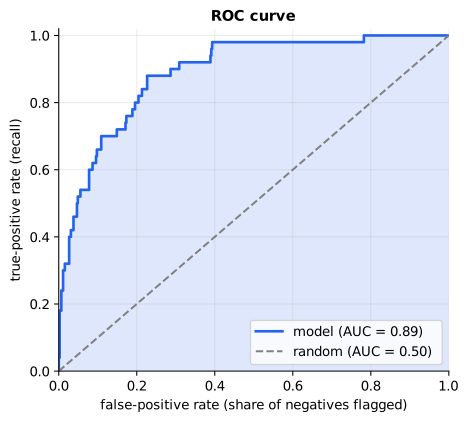
Reading it: the solid line is the ROC curve of synthetic_scores()
(positives shifted 1.5 standard deviations above negatives); the dashed
diagonal is a coin flip. The shaded area is the AUC, about 0.89: pick one
fraud and one legitimate transaction at random and the model scores the
fraud higher 89% of the time. Where the curve bends is where a sensible
threshold lives.
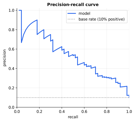
Reading it: the same scores, viewed as precision (y) against recall (x). Moving right means lowering the threshold: you find more of the positives, but precision falls as false alarms pile in. The dotted line is the base rate (10% positives), i.e. what flagging at random achieves. On rare-event problems this plot tells the truth that ROC's tiny false-positive rates hide: at 80% recall only about a third of the flags are real.
In code: roc_curve takes the walk, roc_auc measures the area under
it with auc_trapezoid, and roc_auc_rank counts correctly ordered pairs
instead; Confusion.fpr is FPR, and pr_curve gives the precision-recall
points.
Why it matters in practice. AUC compares models independently of any threshold. On heavily imbalanced data, look at the precision-recall curve too, because FPR stays tiny even when false alarms swamp the true positives.
3. Picking the threshold: price your errors
Everyday picture. A hospital screening test and a spam filter want opposite things. Missing a disease is terrible, so the screen flags generously; losing an important email is annoying, so the spam filter flags cautiously. Same maths, different prices.
Tiny worked example. With the four scores above (frauds 0.9 and 0.4, legitimate 0.6 and 0.1): if a miss costs 10 and a false alarm costs 1, the cheapest rule is "flag at 0.4 or above", catching both frauds and wrongly flagging one legitimate transaction (total cost 1). If a false alarm costs 10 and a miss 1, the cheapest rule is "flag only 0.9", missing one fraud but raising no false alarms (total cost 1).
Level 3: the formula and its symbols
$$ \text{cost}(t) = c_{\text{FN}} \cdot FN(t) + c_{\text{FP}} \cdot FP(t) \qquad t^* = \arg\min_t \text{cost}(t) $$
Symbols
| Symbol | Meaning here | Shape / range |
|---|---|---|
| $t$ | the threshold: flag items scoring at least t | real |
| $FN(t)$, $FP(t)$ | misses and false alarms at that threshold | whole numbers |
| $c_{\text{FN}}$, $c_{\text{FP}}$ | the price of one miss and of one false alarm | ≥ 0 |
| $\arg\min_t$ | "the value of t that makes this smallest" | |
| $t^*$ | the best threshold | real |
In words: the total cost at a threshold is misses times their price plus false alarms times theirs; pick the threshold where that total is lowest.
On the worked example: c_FN = 10, c_FP = 1: at t = 0.4, FN = 0 and FP = 1, cost 1, the minimum. The other thresholds cost 10 (t = 0.9, one miss), 11 (t = 0.6, one miss and one false alarm) and 2 (t = 0.1, two false alarms).
Level 3: in Python
In Python:
frauds, legit = [0.9, 0.4], [0.6, 0.1]
c_FN, c_FP = 10, 1
def cost(t):
    # frauds below t are missed
    FN = sum(s < t for s in frauds)
    # legitimate ones at or above t are false alarms
    FP = sum(s >= t for s in legit)
    return c_FN * FN + c_FP * FP
[cost(t) for t in (0.9, 0.6, 0.4, 0.1)]  # → [10, 11, 1, 2]
# t* = argmin_t cost(t)
min((0.9, 0.6, 0.4, 0.1), key=cost)  # → 0.4
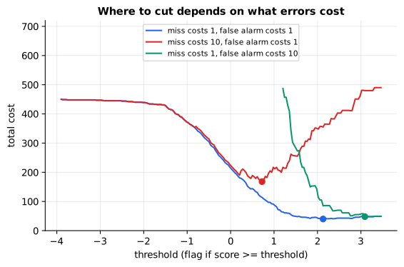
Reading it: each line is the total cost (misses × their price + false alarms × their price) at every threshold, and each dot marks that line's minimum. When a miss costs 10× a false alarm, the best threshold slides left (flag more, higher recall); when a false alarm costs 10×, it slides right (flag less, higher precision). The model is the same in all three lines; only the business decides where to cut.
In code: best_threshold_by_cost tries every distinct score as t
(plus "flag nothing") and keeps the cheapest.
4. Retrieval metrics: judging a search result list
Everyday picture. You ask a librarian for books on a topic and get a stack of five. Did the stack include the books that matter (recall)? How much of the stack is useful (precision)? Is a good book on top, or do you dig for it (reciprocal rank)? Are the best books nearest the top (nDCG)?
Tiny worked example. One query. The system returns d7, d3, d9, d1, d4 in that order. The relevant documents are d3 (very relevant, grade 3), d4 (grade 2) and d8 (grade 1, never returned).
- recall@5 = 2 found of 3 relevant = 0.667
- precision@5 = 2 relevant of 5 returned = 0.4
- reciprocal rank = first relevant result at rank 2, so 1/2 = 0.5
- nDCG@5 = 0.560 (worked below)
flowchart LR
  G[Golden set<br/>query + relevant doc ids] --> R[Retriever]
  R --> K[Ranked top-k list]
  K --> RK["recall@k<br/>did we find them?"]
  K --> PK["precision@k<br/>how much noise?"]
  K --> RR[MRR<br/>how high is the first hit?]
  K --> ND["nDCG@k<br/>are the best ones on top?"]
  G --> RK & PK & RR & ND
Reading it: retrieval is evaluated separately from generation. A golden set pairs real queries with the ids of the documents that answer them; the retriever produces a ranked list for each query; four metrics ask four different questions of the same list. Averaging them over the golden set gives numbers you can track every time you change chunking, the embedding model or the reranker.
Level 3: the formula and its symbols
$$ \text{recall@}k = \frac{|\text{relevant} \cap \text{top-}k|}{|\text{relevant}|} \qquad \text{MRR} = \frac{1}{|Q|}\sum_{q \in Q} \frac{1}{\text{rank}_q} \qquad \text{DCG@}k = \sum_{i=1}^{k} \frac{\text{rel}_i}{\log_2(i + 1)} \qquad \text{nDCG@}k = \frac{\text{DCG@}k}{\text{IDCG@}k} $$
Symbols
| Symbol | Meaning here | Shape / range |
|---|---|---|
| $k$ | how many top results you look at | e.g. 5 |
| $\cap$ | "in both": documents that are relevant and in the top k | set |
| $\lvert\cdot\rvert$ | how many items a set holds | |
| $Q$, $q$ | the set of test queries, and one query | |
| $\text{rank}_q$ | position (1 = top) of the first relevant result for query q | 1, 2, … |
| $\text{rel}_i$ | the relevance grade of the result at position i (0 if irrelevant) | e.g. 0 … 3 |
| $\log_2(i + 1)$ | logarithm base 2: how many times you halve i + 1 to reach 1. It grows slowly, so it is a gentle position discount | 1 at rank 1, 1.58 at rank 2 |
| IDCG | "ideal DCG": the DCG of the same grades sorted best-first, so nDCG tops out at 1 |
In words: recall@k is the share of relevant documents found in the top k; MRR averages one-over-the-rank of the first hit; DCG adds each result's grade, discounted by the log of its position; nDCG divides by the best possible DCG.
On the worked example: recall@5 = 2/3 = 0.667; with one query whose first hit is at rank 2, MRR = 1/2 = 0.5. DCG = 3/log₂(3) + 2/log₂(6) = 1.8928 + 0.7737 = 2.6665 (d3 at rank 2, d4 at rank 5). Ideal order d3, d4, d8: IDCG = 3/1 + 2/1.585 + 1/2 = 4.7619. nDCG = 2.6665/4.7619 = 0.560.
Level 3: in Python
In Python:
import math
ranked = ["d7", "d3", "d9", "d1", "d4"]
# relevance grades; missing means 0
rel = {"d3": 3, "d4": 2, "d8": 1}
k = 5
# recall@k
round(len(set(rel) & set(ranked[:k])) / len(rel), 3)  # → 0.667
rank_q = next(i for i, doc in enumerate(ranked, start=1) if doc in rel)
# MRR over a single query
1 / rank_q  # → 0.5
DCG = sum(rel.get(doc, 0) / math.log2(i + 1) for i, doc in enumerate(ranked[:k], start=1))
# the same grades, best first
best = sorted(rel.values(), reverse=True)[:k]
IDCG = sum(g / math.log2(i + 1) for i, g in enumerate(best, start=1))
print(f"{DCG:.4f} {IDCG:.4f} {DCG / IDCG:.3f}")  # → 2.6665 4.7619 0.560
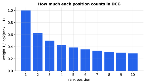
Reading it: the bars are the weight 1/log2(rank + 1) that DCG gives a result at each position. Rank 1 counts fully, rank 2 counts 63%, rank 10 only 29%. That gentle logarithmic decay says "position matters, but a good result at rank 5 is still worth a lot", which matches how people and language models actually use a result list.
In code: recall_at_k and precision_at_k score one ranked list,
reciprocal_rank finds its first hit and mean_reciprocal_rank averages
that over queries; dcg_at_k adds the discounted grades and ndcg_at_k
divides by the ideal ordering's DCG.
Why it matters in practice. For RAG, recall@k (with k = the number of chunks you pass to the model) usually matters most: the model can't use a passage that wasn't retrieved, and no prompt fixes that.
5. Generation metrics: why word overlap misleads
Everyday picture. Grading essays by counting how many words each one shares with the answer key. A student who copies the key's phrasing but gets the key fact wrong scores well; a student who explains it correctly in their own words scores badly.
Tiny worked example. Reference: "The meeting was moved to Friday because the manager is sick."
| candidate | BLEU | ROUGE-L |
|---|---|---|
| "Since the boss is ill, the team rescheduled the meeting for Friday." (correct) | 0.16 | 0.26 |
| "The meeting was moved to Monday because the manager is sick." (wrong) | 0.73 | 0.91 |
BLEU (from machine translation) multiplies together how many of the candidate's 1-, 2-, 3- and 4-word sequences appear in the reference, with a penalty for being too short. ROUGE-L (from summarisation) measures the longest sequence of words the two share in the same order, gaps allowed.
Level 3: the formula and its symbols
$$ \text{BLEU} = \text{BP}\cdot\exp!\Big(\tfrac{1}{4}\sum_{n=1}^{4}\ln p_n\Big) \qquad \text{ROUGE-L} = \frac{2\,P_{\text{LCS}}\,R_{\text{LCS}}}{P_{\text{LCS}} + R_{\text{LCS}}} $$
Symbols
| Symbol | Meaning here | Shape / range |
|---|---|---|
| $p_n$ | share of the candidate's n-word sequences also found in the reference, each counted at most as often as the reference has it | 0 … 1 |
| $\ln$, $\exp$ | natural log and its inverse; exp of the average log is the geometric mean of the four $p_n$ | |
| BP | brevity penalty: 1 if the candidate is longer than the reference, else e^(1 − ref length / candidate length) | 0 … 1 |
| LCS | longest common subsequence: the longest run of words appearing in both texts in the same order | |
| $P_{\text{LCS}}$, $R_{\text{LCS}}$ | LCS length over candidate length, and over reference length | 0 … 1 |
In words: BLEU is the geometric mean of the n-gram match rates, scaled down for short answers; ROUGE-L is the F1 of the longest shared in-order word sequence.
On a hand example: candidate "a b c d", reference "a c d e": the LCS is "a c d", 3 words, so P = 3/4, R = 3/4, ROUGE-L = 0.75. And "the the the the" against "the cat is here" scores unigram precision 1/4: "the" is credited only as often as the reference contains it.
With the numbers: the Monday answer and the reference are both 11
words (full stop and capitals dropped), so BP = 1. It matches 10 of its 11
words, 8 of its 10 word pairs, 6 of its 9 triples and 4 of its 8 four-word
runs. bleu adds 1 to the top and bottom for n ≥ 2 (smoothing, so one
missing four-word run can't zero the score), giving p = 10/11, 9/11, 7/10,
5/9, and BLEU = exp(¼(ln 0.909 + ln 0.818 + ln 0.7 + ln 0.556)) = 0.73.
Its longest shared in-order run is 10 words, so ROUGE-L = 2 · (10/11) ·
(10/11) / (20/11) = 0.91.
Level 3: in Python
In Python:
import math
ref = "the meeting was moved to friday because the manager is sick".split()
cand = "the meeting was moved to monday because the manager is sick".split()
# every run of n words, in order
def grams(words, n):
    return [tuple(words[i:i + n]) for i in range(len(words) - n + 1)]
def p(n):
    c, r = grams(cand, n), grams(ref, n)
    # clipped: at most as often as ref has it
    hits = sum(min(c.count(g), r.count(g)) for g in set(c))
    # add-one smoothing for n ≥ 2
    s = 1 if n > 1 else 0
    return (hits + s) / (len(c) + s)
[round(p(n), 3) for n in range(1, 5)]  # → [0.909, 0.818, 0.7, 0.556]
BP = 1.0 if len(cand) > len(ref) else math.exp(1 - len(ref) / len(cand))
# BLEU
round(BP * math.exp(sum(math.log(p(n)) for n in range(1, 5)) / 4), 2)  # → 0.73
# every word but "monday", in order
P_LCS, R_LCS = 10 / len(cand), 10 / len(ref)
# ROUGE-L
round(2 * P_LCS * R_LCS / (P_LCS + R_LCS), 2)  # → 0.91
# the hand example: LCS "a c d"
P_LCS, R_LCS = 3 / 4, 3 / 4
2 * P_LCS * R_LCS / (P_LCS + R_LCS)  # → 0.75
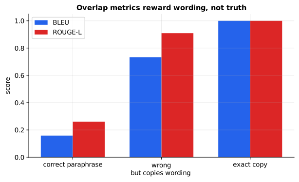
Reading it: three candidate answers to the same reference ("the meeting was moved to Friday because the manager is sick"). The correct paraphrase (left) scores lowest on both metrics; the answer that says Monday (middle) scores nearly as high as an exact copy (right). Overlap metrics reward wording, not truth.
In code: bleu clips each n-gram count, takes the geometric mean and
applies the brevity penalty; rouge_l finds the longest common subsequence
and returns its F1.
Why it matters in practice. Teams grade open-ended output with an LLM as a judge, a model following an explicit rubric, and embedding-based scores like BERTScore do somewhat better than overlap. But a judge must earn trust first (next section).
6. Calibrating a judge: Cohen's kappa
Everyday picture. Two teachers grade the same 20 essays pass/fail and agree on 18. Impressive? Not if 18 of the essays were obvious passes: a careful teacher who reads every essay (and passes those 18) and a lazy one who stamps "pass" on everything without reading would also agree on 18. Cohen's kappa subtracts the agreement you'd expect from luck.
Tiny worked example. Human labels: 18 pass, 2 fail. A lazy judge says "pass" to everything. Raw agreement is 90%, and chance agreement (both say pass at their own rates) is also 0.9 × 1.0 + 0.1 × 0 = 90%, so kappa = 0. A second example: labels (y, y, n, n) vs. (y, n, n, n) agree 3/4 of the time; chance predicts 0.5 × 0.25 + 0.5 × 0.75 = 0.5; kappa = 0.5.
Level 3: the formula and its symbols
$$ \kappa = \frac{p_o - p_e}{1 - p_e} \qquad p_e = \sum_{\ell} p_A(\ell)\, p_B(\ell) $$
Symbols
| Symbol | Meaning here | Shape / range |
|---|---|---|
| $\kappa$ | kappa: agreement beyond chance | ≤ 1; 0 = chance, 1 = perfect |
| $p_o$ | observed agreement: share of items both raters labelled the same | 0 … 1 |
| $p_e$ | agreement expected by chance | 0 … 1 |
| $\ell$ | one possible label (pass, fail…) | |
| $p_A(\ell)$, $p_B(\ell)$ | how often rater A (and rater B) uses label ℓ | 0 … 1 |
In words: kappa is how far agreement beats chance, as a share of the most it could beat chance by.
On the worked example: p_o = 0.75, p_e = 0.5, κ = (0.75 − 0.5)/(1 − 0.5) = 0.5.
Level 3: in Python
In Python:
# rater A's labels
A = ["y", "y", "n", "n"]
# rater B's labels
B = ["y", "n", "n", "n"]
p_o = sum(a == b for a, b in zip(A, B)) / len(A)
# Σ_ℓ p_A(ℓ) p_B(ℓ)
p_e = sum((A.count(ell) / len(A)) * (B.count(ell) / len(B)) for ell in ("y", "n"))
p_o, p_e  # → (0.75, 0.5)
# κ
(p_o - p_e) / (1 - p_e)  # → 0.5
flowchart LR
  S[Sample of real outputs] --> H[Humans label<br/>pass / fail]
  S --> J[LLM judge + rubric<br/>labels pass / fail]
  H --> K[Cohen's kappa]
  J --> K
  K -->|kappa high enough| U[Use the judge at scale]
  K -->|too low| F[Fix rubric, examples<br/>or judge model]
  F --> J
Reading it: the judge earns trust the same way a new human reviewer would: grade a sample that people have already graded and compare. Kappa, not raw agreement, is the gate, because on a sample that is mostly "pass" a lazy judge agrees by accident. Only once the judge clears the bar do you let it grade thousands of outputs, and you repeat the check whenever the judge model or rubric changes.
In code: cohens_kappa computes p_o and p_e from two lists of labels
and returns κ.
Why it matters in practice. Kappa above about 0.6 is usually considered substantial agreement. Re-check it whenever the judge model or rubric changes.
In 20 seconds
- Precision: of what I flagged, how much was right. Recall: of what mattered, how much I found. F1 balances them.
- Accuracy lies on imbalanced data. Flagging nothing on 1% fraud scores 99%.
- ROC-AUC is the probability a random positive outranks a random negative.
- Choose the threshold by what each kind of error costs.
- For RAG, measure recall@k first. What isn't retrieved can't be used.
- BLEU/ROUGE punish correct paraphrases; use an LLM judge and calibrate it against humans with Cohen's kappa.
Self-test questions
Q: A fraud model has 94% accuracy. Is it good? A: You can't tell from accuracy. If fraud is 10% of traffic, check recall and precision. In the worked example recall is only 60%, so 4 in 10 frauds slip through.
Q: When do you optimize for precision vs. recall? A: By the cost of each error. If a miss is expensive (fraud, cancer screening, a relevant legal document), favor recall. If a false alarm is expensive (blocking a good customer, paging an engineer at 3 a.m.), favor precision. Set the threshold to minimize expected cost.
Q: What does an AUC of 0.8 mean? A: A randomly chosen positive gets a higher score than a randomly chosen negative 80% of the time. It measures ranking quality across all thresholds; 0.5 is random.
Q: Which retrieval metric matters most for RAG, and why? A: Recall@k, where k is the number of chunks you pass to the model. If the right passage isn't in the top k, no prompt engineering can recover the answer. Add MRR or nDCG when position within the context matters.
Q: Why not grade LLM answers with BLEU or ROUGE? A: They measure surface overlap with one reference. A correct paraphrase scores low and a wrong answer that reuses the reference's words scores high. Use code-based checks where possible and a rubric-driven LLM judge otherwise, validated against human labels.
Q: Your LLM judge agrees with humans 90% of the time. Good enough? A: Not necessarily. If 90% of answers are "pass", a judge that always says "pass" also agrees 90%. Compute Cohen's kappa to correct for chance agreement.
The papers behind this lesson
- Zheng et al., Judging LLM-as-a-Judge with MT-Bench and Chatbot Arena (2023): https://arxiv.org/abs/2306.05685. Measured how well strong language models agree with human preferences when used as judges, and catalogued their biases (position, verbosity, self-preference). annotated companion
- Papineni et al., BLEU: a Method for Automatic Evaluation of Machine Translation (2002): https://aclanthology.org/P02-1040/. Introduced clipped n-gram precision with a brevity penalty.
- Lin, ROUGE: A Package for Automatic Evaluation of Summaries (2004): https://aclanthology.org/W04-1013/. Introduced recall-oriented overlap measures, including the LCS-based ROUGE-L.
- Zhang et al., BERTScore: Evaluating Text Generation with BERT (2019): https://arxiv.org/abs/1904.09675. Compared candidate and reference by embedding similarity rather than exact word overlap.
Further reading
- scikit-learn, Metrics and scoring: https://scikit-learn.org/stable/modules/model_evaluation.html
- Receiver operating characteristic (Wikipedia): https://en.wikipedia.org/wiki/Receiver_operating_characteristic
- Discounted cumulative gain (Wikipedia): https://en.wikipedia.org/wiki/Discounted_cumulative_gain
- Cohen's kappa (Wikipedia): https://en.wikipedia.org/wiki/Cohen%27s_kappa
1r""" 2# Metrics: how you know whether a model is any good 3 4Run: `python -m primer.ml.metrics` 5 6New to the notation? `primer.notation` explains every symbol used here from 7zero. 8 9## Level 1: The practitioner's guide 10 11**In one sentence.** A metric is the number you use to decide whether a 12model is good enough, as opposed to the loss the model optimises 13(`primer.ml.losses`), and every metric answers exactly one question while 14staying silent on all the others. 15 16**When you need it.** Every time a number decides something: whether a 17model ships, which of two retrievers your RAG system keeps, whether an 18automated judge may replace human review. The tell that you have the wrong 19metric is a number that looks great offline and a system that disappoints. 20This lesson's fraud detector has 94% accuracy and misses 4 frauds in 10; on 21traffic that is 1% fraud, a model that flags nothing scores 99% accuracy 22with recall 0. Its generation example is starker: against the reference 23"the meeting was moved to Friday because the manager is sick", the answer 24that says Monday scores BLEU 0.73 and ROUGE-L 0.91, and the correct 25paraphrase scores 0.16 and 0.26. And a judge that stamps "pass" on 26everything agrees with humans 90% of the time on a sample that is 90% 27passes, with a Cohen's kappa of exactly 0. You do not need this lesson to 28read a training curve; that is the loss. You need it the moment a number 29leaves the training loop and enters a decision. 30 31**Your options.** By the question they answer: 32 33| Metric | The question it answers | What it hides | What it needs | Where it lives | 34|---|---|---|---|---| 35| Accuracy | Of all decisions, what share were right? | Class imbalance: flag nothing on 1% fraud and score 99% | Labels and a threshold | Balanced classification only | 36| Precision, recall, F1 | Of what I flagged, how much was right; of what mattered, how much I found; F1 balances the two | The threshold that produced them, and that F1 prices a miss and a false alarm equally | Labels and a threshold | Every fraud, spam and moderation filter | 37| ROC-AUC | Across every threshold, how often does a random positive outrank a random negative? | On rare events, false alarms can swamp the true positives while the false-positive rate stays tiny | Scores and labels | Comparing models before a threshold is chosen | 38| Precision-recall curve | At each level of recall, what share of the flags are real? | Nothing about ranking below the recall you care about | Scores and labels | Rare-event problems | 39| Cost-weighted threshold | Which cut-off makes misses times their price plus false alarms times theirs smallest? | It needs the prices, which only the business knows | Two prices | The decision itself | 40| recall@k, precision@k, MRR, nDCG@k | Did we find the relevant documents, how much noise came with them, how high is the first hit, are the best ones on top? | Anything the golden set does not cover; nDCG needs graded relevance | A golden set: queries with the ids of the documents that answer them | Search and RAG retrieval | 41| BLEU, ROUGE-L | How much wording does the answer share with a reference? | Truth: a correct paraphrase scores near zero | One or more reference answers | Machine translation, summarisation, legacy pipelines | 42| Embedding similarity (BERTScore) | How close in meaning is the answer to a reference? | It still needs a reference, and closeness is not correctness | A reference and an embedding model | Generation with references | 43| LLM judge, calibrated with Cohen's kappa | Does a rubric-following model agree with human graders beyond chance? | The judge's own biases (position, verbosity, self-enhancement) and chance agreement | A human-labelled sample and a rubric | Open-ended generation and agent evaluation | 44 45**How to choose.** Name the question first, then the metric that answers 46it. 47 48- A classifier with a threshold in production: report precision and recall 49 at that threshold, and pick the threshold by pricing the two errors. In 50 this lesson, pricing a miss at 10 and a false alarm at 1 drops the 51 threshold and lifts recall from 0.30 to 0.88; the reverse prices raise it 52 until precision is 1.00. Never lead with accuracy on imbalanced data. 53- Comparing models before any threshold exists: ROC-AUC. If positives are 54 rare, look at the precision-recall curve as well. 55- Retrieval, including the retrieval half of RAG: recall@k with k set to 56 the number of chunks you actually pass to the model, because the model 57 cannot use what was not retrieved. Add MRR or nDCG when position matters. 58- Generation: a code-based check wherever the answer can be verified (a 59 test passes, a number matches, the JSON parses). Overlap metrics only 60 where the task is nearly verbatim, such as translation. Everything else, 61 an LLM judge with a written rubric, calibrated against people with kappa 62 before it grades anything at scale. 63- Whatever you pick, a metric is meaningless without its conditions: the 64 threshold, the k, the golden set, the sample the judge was checked on. 65 Report them next to the number, every time. 66 67**What it costs.** Metrics cost labels, not compute. Classification needs 68labelled examples and, for the threshold, two prices you must extract from 69whoever owns the consequences. Retrieval needs a golden set of real queries 70paired with the documents that answer them, which is hours of a 71knowledgeable person's time and the single best investment in a RAG system, 72because you can then rerun recall@k after every change to chunking, the 73embedding model or the reranker. Generation costs the most: reference 74answers for overlap metrics, or human labels for the sample a judge is 75calibrated on, plus a model call per graded output for the judge itself, 76and the calibration is repeated every time the judge model or the rubric 77changes. The cost of the wrong metric is the one that matters: it is the 78gap between the dashboard's 94% and the four frauds in ten that walked 79through. 80 81**What breaks.** 82 83- **Accuracy on imbalanced data.** 99% for a model that does nothing. Use 84 precision and recall. 85- **A number with no threshold.** "What's the accuracy?" is incomplete 86 without "at what threshold?"; every classification metric changes when 87 the cut-off moves. 88- **AUC on rare events.** This lesson's classifier has an AUC of 0.89 and, 89 at 80% recall, only about a third of its flags are real against a 10% 90 base rate. Read the precision-recall curve. 91- **F1 when the errors cost differently.** The harmonic mean pulls toward 92 the smaller of the two: precision 1.0 with recall 0.1 gives F1 0.18. If a 93 miss costs ten times a false alarm, F1 is the wrong target; price the 94 errors instead. 95- **recall@k at the wrong k.** Recall@20 is no comfort when you pass five 96 chunks to the model. Measure at the k you serve. 97- **Overlap metrics on paraphrase.** The Monday answer, factually wrong, 98 scores 0.91 on ROUGE-L. Overlap measures wording, not truth. 99- **Raw agreement for a judge.** 90% agreement and kappa 0 describe the 100 same lazy judge. Kappa above about 0.6 is usually read as substantial 101 agreement; below it, fix the rubric, the examples or the judge model. 102- **A judge that drifts.** A new judge model or an edited rubric is a new 103 judge. Re-run the calibration. 104 105**In the wild.** scikit-learn ships the classification family as 106`precision_score`, `recall_score`, `f1_score`, `roc_auc_score`, 107`average_precision_score` and `cohen_kappa_score`, and its metrics guide is 108in Further reading. In retrieval, the BEIR benchmark (Thakur et al., 2021) 109compares lexical, sparse, dense, late-interaction and reranking systems 110across 18 datasets. BLEU (Papineni et al., 2002) and ROUGE (Lin, 2004) are 111still the reported numbers in translation and summarisation, with BERTScore 112(Zhang et al., 2019) as the embedding-based successor. For judging, Zheng 113et al. (2023) found that strong LLM judges reach over 80% agreement with 114humans on MT-Bench, the level humans reach with each other, and named the 115position, verbosity and self-enhancement biases every judge pipeline now 116guards against. `primer.agents.evals` turns these metrics into a release 117gate for an agent. 118 119**Go deeper.** Level 2 builds each family from a hand-sized example: the 120four cells of the confusion matrix and the accuracy trap, the ROC curve as a 121walk whose area counts correctly ordered pairs, the cheapest threshold under 122two prices, the four retrieval metrics on one five-document list, BLEU and 123ROUGE-L on the Monday sentence, and Cohen's kappa on twenty essays. If you 124only needed to pick the metric and read it honestly, you are done. 125 126## Level 2: How it works, from scratch 127 128A loss function is what the model *optimizes* during training; a metric is 129what *you* use to decide whether it's working. Picking the wrong metric is 130one of the most common ways a project looks great offline and fails in 131production. This lesson builds every metric from scratch in three families: 132 1331. **Classification:** precision, recall, F1, accuracy, the confusion 134 matrix, ROC-AUC, precision-recall curves, and choosing a threshold by the 135 *cost* of each kind of error. 1362. **Retrieval:** recall@k, precision@k, MRR and nDCG, the metrics for search 137 and retrieval-augmented generation (RAG). 1383. **Generation:** BLEU and ROUGE-L (word overlap), why they fail on 139 language-model output, and how to check an automated judge against people 140 with Cohen's kappa. 141 142## 1. Classification: precision, recall and the confusion matrix 143 144**Everyday picture.** You're fishing for trout in a lake that also holds old 145boots. **Precision** asks: of everything in your net, how much is trout? 146**Recall** asks: of all the trout in the lake, how many did you catch? A tiny 147net held in one good spot has high precision and low recall; dragging a huge 148net across the whole lake has high recall and a lot of boots. 149 150**Tiny worked example: fraud detection.** Of 100 transactions, 10 are fraud. 151The model flags 8, and 6 of those are truly fraud. So 6 hits (true 152positives, TP), 2 false alarms (false positives, FP), 4 misses (false 153negatives, FN) and 88 correct passes (true negatives, TN). 154 155| Metric | Calculation | Result | 156|-----------|---------------------------------|--------| 157| Precision | 6 correct ÷ 8 flagged | 75% | 158| Recall | 6 found ÷ 10 actual fraud | 60% | 159| F1 | 2 × 0.75 × 0.60 ÷ (0.75 + 0.60) | 67% | 160| Accuracy | (6 + 88 correct) ÷ 100 | 94% | 161 162Accuracy looks great at 94% while the model misses 4 in 10 frauds. 163 164```mermaid 165flowchart LR 166 X[Item] --> M[Model] 167 M --> S[Score<br/>e.g. 0.73] 168 S --> T{Score >= threshold?} 169 T -->|yes| P[Flagged positive] 170 T -->|no| N[Not flagged] 171 P --> CM[Confusion matrix<br/>TP / FP / FN / TN] 172 N --> CM 173 L[True label] --> CM 174 CM --> MET[Precision, recall,<br/>F1, accuracy] 175``` 176 177**Reading it:** a classifier never outputs "fraud" directly; it outputs a 178*score*, and a threshold that *you* choose turns scores into decisions. 179Comparing each decision with the true label drops the item into one of four 180cells of the confusion matrix, and every classification metric is just a 181ratio of those four counts. Change the threshold and every metric changes, 182which is why "what's the accuracy?" is incomplete without "at what 183threshold?". 184 185| | predicted positive | predicted negative | 186|-----------------|--------------------|--------------------| 187| actual positive | TP = 6 | FN = 4 (missed) | 188| actual negative | FP = 2 (false alarm) | TN = 88 | 189 190$$ 191\text{precision} = \frac{TP}{TP + FP} \qquad 192\text{recall} = \frac{TP}{TP + FN} \qquad 193F_1 = \frac{2PR}{P + R} \qquad 194\text{accuracy} = \frac{TP + TN}{N} 195$$ 196 197**Symbols** 198 199| Symbol | Meaning here | Shape / range | 200|---|---|---| 201| TP, FP, FN, TN | counts of hits, false alarms, misses and correct passes | whole numbers | 202| $P$, $R$ | precision and recall | 0 … 1 | 203| $F_1$ | the **harmonic mean** of P and R: an average that is dragged towards the smaller of the two | 0 … 1 | 204| $N$ | total number of items, TP + FP + FN + TN | whole number | 205| fraction bar | "divided by" | | 206 207**In words:** precision is hits over everything flagged; recall is hits over 208everything that should have been flagged; F1 is twice their product over 209their sum; accuracy is everything right over everything. 210 211**On the worked example:** P = 6/(6 + 2) = 0.75; R = 6/(6 + 4) = 0.60; 212F1 = 2 × 0.75 × 0.60 / 1.35 = 0.667; accuracy = (6 + 88)/100 = 0.94. The 213harmonic mean punishes imbalance: P = 1.0 with R = 0.1 gives F1 = 0.18, not 214the ordinary average of 0.55. 215 216**In Python:** 217 218```python 219TP, FP, FN, TN = 6, 2, 4, 88 220N = TP + FP + FN + TN 221# precision, recall 222P, R = TP / (TP + FP), TP / (TP + FN) 223P, R # → (0.75, 0.6) 224# F1, accuracy 225round(2 * P * R / (P + R), 3), (TP + TN) / N # → (0.667, 0.94) 226# F1 when P = 1.0 and R = 0.1 227round(2 * 1.0 * 0.1 / (1.0 + 0.1), 2) # → 0.18 228``` 229 230**In code:** `confusion` sorts labels and decisions into a `Confusion`, 231whose `Confusion.precision`, `Confusion.recall`, `Confusion.f1` and 232`Confusion.accuracy` are the four formulas. `fraud_example` rebuilds the 233100 transactions above, and `flag_nothing_trap` builds the model below that 234never flags anything. 235 236**Why it matters in practice: the accuracy trap.** If 1% of transactions are 237fraud, a model that flags *nothing* is 99% accurate and completely useless 238(recall 0). On imbalanced data, never lead with accuracy. 239 240## 2. ROC-AUC: how well does the model *rank*? 241 242**Everyday picture.** A smoke alarm has a sensitivity dial. Turn it up and 243it catches every fire but also shrieks at toast; turn it down and it stays 244quiet but might miss a real fire. The ROC curve draws *every* dial setting 245at once, and AUC scores the alarm across all of them. 246 247**Tiny worked example.** Two frauds scored 0.9 and 0.4, two legitimate 248transactions scored 0.6 and 0.1. Compare every (fraud, legitimate) pair: 2490.9 > 0.6 ✓, 0.9 > 0.1 ✓, 0.4 > 0.6 ✗, 0.4 > 0.1 ✓. Three of four pairs are 250ranked correctly, so **AUC = 0.75**. 251 252```mermaid 253flowchart TD 254 A[Sort items by score, highest first] --> B[Start with threshold above every score<br/>nothing flagged: point 0,0] 255 B --> C[Lower the threshold past the next distinct score] 256 C --> D{Which items became flagged?} 257 D -->|a positive| E[Step up: TPR rises] 258 D -->|a negative| F[Step right: FPR rises] 259 D -->|a tie of both| G[Diagonal step: half credit] 260 E --> H{Everything flagged?} 261 F --> H 262 G --> H 263 H -->|no| C 264 H -->|yes| I[End at point 1,1<br/>AUC = area under the path] 265``` 266 267**Reading it:** the ROC curve is a walk. Starting from "flag nothing" 268(bottom-left) you lower the threshold one score at a time; each positive you 269pick up moves you up, each negative moves you right. A perfect ranker goes 270straight up then straight right (area 1.0); a random one wanders along the 271diagonal (area 0.5). Because the walk moves *up* exactly when a positive 272outranks the remaining negatives, the area counts correctly ordered 273(positive, negative) pairs, which is why AUC equals the pairwise win rate. 274The code computes AUC both ways (trapezoids under the curve, and counting 275pairs) and they agree exactly. 276 277$$ 278\text{TPR} = \frac{TP}{TP + FN} \qquad 279\text{FPR} = \frac{FP}{FP + TN} \qquad 280\text{AUC} = \frac{1}{|P|\,|N|}\sum_{p \in P}\sum_{n \in N}\Big([s_p > s_n] + \tfrac{1}{2}[s_p = s_n]\Big) 281$$ 282 283**Symbols** 284 285| Symbol | Meaning here | Shape / range | 286|---|---|---| 287| TPR | true-positive rate: recall, the share of positives flagged | 0 … 1 | 288| FPR | false-positive rate: the share of negatives wrongly flagged | 0 … 1 | 289| $P$, $N$ (in the AUC sum) | the set of positive items and the set of negative items | sets | 290| $\lvert P \rvert$, $\lvert N \rvert$ | how many items each set holds | whole numbers | 291| $s_p$, $s_n$ | the model's score for positive p and negative n | real | 292| $[\ldots]$ | 1 if the statement inside is true, else 0 | 0 or 1 | 293| $\sum_{p \in P}\sum_{n \in N}$ | add over every (positive, negative) pair | | 294 295**In words:** AUC is the share of (positive, negative) pairs in which the 296positive gets the higher score, counting ties as half. 297 298**On the worked example:** 2 positives × 2 negatives = 4 pairs; 3 are 299ordered correctly; AUC = 3/4 = 0.75. One point on the curve: at threshold 3000.5 the model flags the 0.9 fraud and the 0.6 legitimate transaction, so 301TPR = 1/(1 + 1) = 0.5 and FPR = 1/(1 + 1) = 0.5. 302 303**In Python:** 304 305```python 306# scores of the positives (frauds) 307s_P = [0.9, 0.4] 308# scores of the negatives (legitimate) 309s_N = [0.6, 0.1] 310t = 0.5 311TP, FN = sum(s >= t for s in s_P), sum(s < t for s in s_P) 312FP, TN = sum(s >= t for s in s_N), sum(s < t for s in s_N) 313# TPR, FPR 314TP / (TP + FN), FP / (FP + TN) # → (0.5, 0.5) 315pairs = sum((s_p > s_n) + 0.5 * (s_p == s_n) for s_p in s_P for s_n in s_N) 316# AUC: the share of pairs ranked correctly 317pairs / (len(s_P) * len(s_N)) # → 0.75 318``` 319 320 321 322**Reading it:** the solid line is the ROC curve of `synthetic_scores()` 323(positives shifted 1.5 standard deviations above negatives); the dashed 324diagonal is a coin flip. The shaded area is the AUC, about 0.89: pick one 325fraud and one legitimate transaction at random and the model scores the 326fraud higher 89% of the time. Where the curve bends is where a sensible 327threshold lives. 328 329 330 331**Reading it:** the same scores, viewed as precision (y) against recall (x). 332Moving right means lowering the threshold: you find more of the positives, 333but precision falls as false alarms pile in. The dotted line is the base 334rate (10% positives), i.e. what flagging at random achieves. On rare-event 335problems this plot tells the truth that ROC's tiny false-positive *rates* 336hide: at 80% recall only about a third of the flags are real. 337 338**In code:** `roc_curve` takes the walk, `roc_auc` measures the area under 339it with `auc_trapezoid`, and `roc_auc_rank` counts correctly ordered pairs 340instead; `Confusion.fpr` is FPR, and `pr_curve` gives the precision-recall 341points. 342 343**Why it matters in practice.** AUC compares models independently of any 344threshold. On heavily imbalanced data, look at the precision-recall curve 345too, because FPR stays tiny even when false alarms swamp the true positives. 346 347## 3. Picking the threshold: price your errors 348 349**Everyday picture.** A hospital screening test and a spam filter want 350opposite things. Missing a disease is terrible, so the screen flags 351generously; losing an important email is annoying, so the spam filter flags 352cautiously. Same maths, different prices. 353 354**Tiny worked example.** With the four scores above (frauds 0.9 and 0.4, 355legitimate 0.6 and 0.1): if a miss costs 10 and a false alarm costs 1, the 356cheapest rule is "flag at 0.4 or above", catching both frauds and wrongly 357flagging one legitimate transaction (total cost **1**). If a false alarm 358costs 10 and a miss 1, the cheapest rule is "flag only 0.9", missing one 359fraud but raising no false alarms (total cost **1**). 360 361$$ 362\text{cost}(t) = c_{\text{FN}} \cdot FN(t) + c_{\text{FP}} \cdot FP(t) \qquad t^* = \arg\min_t \text{cost}(t) 363$$ 364 365**Symbols** 366 367| Symbol | Meaning here | Shape / range | 368|---|---|---| 369| $t$ | the threshold: flag items scoring at least t | real | 370| $FN(t)$, $FP(t)$ | misses and false alarms at that threshold | whole numbers | 371| $c_{\text{FN}}$, $c_{\text{FP}}$ | the price of one miss and of one false alarm | ≥ 0 | 372| $\arg\min_t$ | "the value of t that makes this smallest" | | 373| $t^*$ | the best threshold | real | 374 375**In words:** the total cost at a threshold is misses times their price 376plus false alarms times theirs; pick the threshold where that total is 377lowest. 378 379**On the worked example:** c_FN = 10, c_FP = 1: at t = 0.4, FN = 0 and 380FP = 1, cost 1, the minimum. The other thresholds cost 10 (t = 0.9, one 381miss), 11 (t = 0.6, one miss and one false alarm) and 2 (t = 0.1, two false 382alarms). 383 384**In Python:** 385 386```python 387frauds, legit = [0.9, 0.4], [0.6, 0.1] 388c_FN, c_FP = 10, 1 389def cost(t): 390 # frauds below t are missed 391 FN = sum(s < t for s in frauds) 392 # legitimate ones at or above t are false alarms 393 FP = sum(s >= t for s in legit) 394 return c_FN * FN + c_FP * FP 395[cost(t) for t in (0.9, 0.6, 0.4, 0.1)] # → [10, 11, 1, 2] 396# t* = argmin_t cost(t) 397min((0.9, 0.6, 0.4, 0.1), key=cost) # → 0.4 398``` 399 400 401 402**Reading it:** each line is the total cost (misses × their price + false 403alarms × their price) at every threshold, and each dot marks that line's 404minimum. When a miss costs 10× a false alarm, the best threshold slides left 405(flag more, higher recall); when a false alarm costs 10×, it slides right 406(flag less, higher precision). The model is the same in all three lines; 407only the business decides where to cut. 408 409**In code:** `best_threshold_by_cost` tries every distinct score as t 410(plus "flag nothing") and keeps the cheapest. 411 412## 4. Retrieval metrics: judging a search result list 413 414**Everyday picture.** You ask a librarian for books on a topic and get a 415stack of five. Did the stack include the books that matter (recall)? How 416much of the stack is useful (precision)? Is a good book on top, or do you 417dig for it (reciprocal rank)? Are the *best* books nearest the top (nDCG)? 418 419**Tiny worked example.** One query. The system returns d7, d3, d9, d1, d4 in 420that order. The relevant documents are d3 (very relevant, grade 3), d4 421(grade 2) and d8 (grade 1, never returned). 422 423* recall@5 = 2 found of 3 relevant = **0.667** 424* precision@5 = 2 relevant of 5 returned = **0.4** 425* reciprocal rank = first relevant result at rank 2, so 1/2 = **0.5** 426* nDCG@5 = **0.560** (worked below) 427 428```mermaid 429flowchart LR 430 G[Golden set<br/>query + relevant doc ids] --> R[Retriever] 431 R --> K[Ranked top-k list] 432 K --> RK["recall@k<br/>did we find them?"] 433 K --> PK["precision@k<br/>how much noise?"] 434 K --> RR[MRR<br/>how high is the first hit?] 435 K --> ND["nDCG@k<br/>are the best ones on top?"] 436 G --> RK & PK & RR & ND 437``` 438 439**Reading it:** retrieval is evaluated *separately* from generation. A 440golden set pairs real queries with the ids of the documents that answer 441them; the retriever produces a ranked list for each query; four metrics ask 442four different questions of the same list. Averaging them over the golden 443set gives numbers you can track every time you change chunking, the 444embedding model or the reranker. 445 446$$ 447\text{recall@}k = \frac{|\text{relevant} \cap \text{top-}k|}{|\text{relevant}|} \qquad 448\text{MRR} = \frac{1}{|Q|}\sum_{q \in Q} \frac{1}{\text{rank}_q} \qquad 449\text{DCG@}k = \sum_{i=1}^{k} \frac{\text{rel}_i}{\log_2(i + 1)} \qquad 450\text{nDCG@}k = \frac{\text{DCG@}k}{\text{IDCG@}k} 451$$ 452 453**Symbols** 454 455| Symbol | Meaning here | Shape / range | 456|---|---|---| 457| $k$ | how many top results you look at | e.g. 5 | 458| $\cap$ | "in both": documents that are relevant *and* in the top k | set | 459| $\lvert\cdot\rvert$ | how many items a set holds | | 460| $Q$, $q$ | the set of test queries, and one query | | 461| $\text{rank}_q$ | position (1 = top) of the first relevant result for query q | 1, 2, … | 462| $\text{rel}_i$ | the relevance grade of the result at position i (0 if irrelevant) | e.g. 0 … 3 | 463| $\log_2(i + 1)$ | logarithm base 2: how many times you halve i + 1 to reach 1. It grows slowly, so it is a gentle position discount | 1 at rank 1, 1.58 at rank 2 | 464| IDCG | "ideal DCG": the DCG of the same grades sorted best-first, so nDCG tops out at 1 | | 465 466**In words:** recall@k is the share of relevant documents found in the top 467k; MRR averages one-over-the-rank of the first hit; DCG adds each result's 468grade, discounted by the log of its position; nDCG divides by the best 469possible DCG. 470 471**On the worked example:** recall@5 = 2/3 = 0.667; with one query whose 472first hit is at rank 2, MRR = 1/2 = 0.5. DCG = 3/log₂(3) + 2/log₂(6) = 4731.8928 + 0.7737 = 2.6665 (d3 at rank 2, d4 at rank 5). Ideal order d3, d4, 474d8: IDCG = 3/1 + 2/1.585 + 1/2 = 4.7619. nDCG = 2.6665/4.7619 = 0.560. 475 476**In Python:** 477 478```python 479import math 480ranked = ["d7", "d3", "d9", "d1", "d4"] 481# relevance grades; missing means 0 482rel = {"d3": 3, "d4": 2, "d8": 1} 483k = 5 484# recall@k 485round(len(set(rel) & set(ranked[:k])) / len(rel), 3) # → 0.667 486rank_q = next(i for i, doc in enumerate(ranked, start=1) if doc in rel) 487# MRR over a single query 4881 / rank_q # → 0.5 489DCG = sum(rel.get(doc, 0) / math.log2(i + 1) for i, doc in enumerate(ranked[:k], start=1)) 490# the same grades, best first 491best = sorted(rel.values(), reverse=True)[:k] 492IDCG = sum(g / math.log2(i + 1) for i, g in enumerate(best, start=1)) 493print(f"{DCG:.4f} {IDCG:.4f} {DCG / IDCG:.3f}") # → 2.6665 4.7619 0.560 494``` 495 496 497 498**Reading it:** the bars are the weight 1/log2(rank + 1) that DCG gives a 499result at each position. Rank 1 counts fully, rank 2 counts 63%, rank 10 500only 29%. That gentle logarithmic decay says "position matters, but a good 501result at rank 5 is still worth a lot", which matches how people and 502language models actually use a result list. 503 504**In code:** `recall_at_k` and `precision_at_k` score one ranked list, 505`reciprocal_rank` finds its first hit and `mean_reciprocal_rank` averages 506that over queries; `dcg_at_k` adds the discounted grades and `ndcg_at_k` 507divides by the ideal ordering's DCG. 508 509**Why it matters in practice.** For RAG, recall@k (with k = the number of 510chunks you pass to the model) usually matters most: the model can't use a 511passage that wasn't retrieved, and no prompt fixes that. 512 513## 5. Generation metrics: why word overlap misleads 514 515**Everyday picture.** Grading essays by counting how many words each one 516shares with the answer key. A student who copies the key's phrasing but gets 517the key fact wrong scores well; a student who explains it correctly in their 518own words scores badly. 519 520**Tiny worked example.** Reference: "The meeting was moved to Friday because 521the manager is sick." 522 523| candidate | BLEU | ROUGE-L | 524|---|---|---| 525| "Since the boss is ill, the team rescheduled the meeting for Friday." (correct) | 0.16 | 0.26 | 526| "The meeting was moved to *Monday* because the manager is sick." (wrong) | 0.73 | 0.91 | 527 528**BLEU** (from machine translation) multiplies together how many of the 529candidate's 1-, 2-, 3- and 4-word sequences appear in the reference, with a 530penalty for being too short. **ROUGE-L** (from summarisation) measures the 531longest sequence of words the two share in the same order, gaps allowed. 532 533$$ 534\text{BLEU} = \text{BP}\cdot\exp\!\Big(\tfrac{1}{4}\sum_{n=1}^{4}\ln p_n\Big) \qquad 535\text{ROUGE-L} = \frac{2\,P_{\text{LCS}}\,R_{\text{LCS}}}{P_{\text{LCS}} + R_{\text{LCS}}} 536$$ 537 538**Symbols** 539 540| Symbol | Meaning here | Shape / range | 541|---|---|---| 542| $p_n$ | share of the candidate's n-word sequences also found in the reference, each counted at most as often as the reference has it | 0 … 1 | 543| $\ln$, $\exp$ | natural log and its inverse; exp of the average log is the *geometric mean* of the four $p_n$ | | 544| BP | brevity penalty: 1 if the candidate is longer than the reference, else e^(1 − ref length / candidate length) | 0 … 1 | 545| LCS | longest common subsequence: the longest run of words appearing in both texts in the same order | | 546| $P_{\text{LCS}}$, $R_{\text{LCS}}$ | LCS length over candidate length, and over reference length | 0 … 1 | 547 548**In words:** BLEU is the geometric mean of the n-gram match rates, scaled 549down for short answers; ROUGE-L is the F1 of the longest shared in-order 550word sequence. 551 552**On a hand example:** candidate "a b c d", reference "a c d e": the LCS is 553"a c d", 3 words, so P = 3/4, R = 3/4, ROUGE-L = 0.75. And "the the the the" 554against "the cat is here" scores unigram precision 1/4: "the" is credited 555only as often as the reference contains it. 556 557**With the numbers:** the *Monday* answer and the reference are both 11 558words (full stop and capitals dropped), so BP = 1. It matches 10 of its 11 559words, 8 of its 10 word pairs, 6 of its 9 triples and 4 of its 8 four-word 560runs. `bleu` adds 1 to the top and bottom for n ≥ 2 (smoothing, so one 561missing four-word run can't zero the score), giving p = 10/11, 9/11, 7/10, 5625/9, and BLEU = exp(¼(ln 0.909 + ln 0.818 + ln 0.7 + ln 0.556)) = **0.73**. 563Its longest shared in-order run is 10 words, so ROUGE-L = 2 · (10/11) · 564(10/11) / (20/11) = **0.91**. 565 566**In Python:** 567 568```python 569import math 570ref = "the meeting was moved to friday because the manager is sick".split() 571cand = "the meeting was moved to monday because the manager is sick".split() 572# every run of n words, in order 573def grams(words, n): 574 return [tuple(words[i:i + n]) for i in range(len(words) - n + 1)] 575def p(n): 576 c, r = grams(cand, n), grams(ref, n) 577 # clipped: at most as often as ref has it 578 hits = sum(min(c.count(g), r.count(g)) for g in set(c)) 579 # add-one smoothing for n ≥ 2 580 s = 1 if n > 1 else 0 581 return (hits + s) / (len(c) + s) 582[round(p(n), 3) for n in range(1, 5)] # → [0.909, 0.818, 0.7, 0.556] 583BP = 1.0 if len(cand) > len(ref) else math.exp(1 - len(ref) / len(cand)) 584# BLEU 585round(BP * math.exp(sum(math.log(p(n)) for n in range(1, 5)) / 4), 2) # → 0.73 586# every word but "monday", in order 587P_LCS, R_LCS = 10 / len(cand), 10 / len(ref) 588# ROUGE-L 589round(2 * P_LCS * R_LCS / (P_LCS + R_LCS), 2) # → 0.91 590# the hand example: LCS "a c d" 591P_LCS, R_LCS = 3 / 4, 3 / 4 5922 * P_LCS * R_LCS / (P_LCS + R_LCS) # → 0.75 593``` 594 595 596 597**Reading it:** three candidate answers to the same reference ("the meeting 598was moved to Friday because the manager is sick"). The correct paraphrase 599(left) scores lowest on both metrics; the answer that says *Monday* (middle) 600scores nearly as high as an exact copy (right). Overlap metrics reward 601wording, not truth. 602 603**In code:** `bleu` clips each n-gram count, takes the geometric mean and 604applies the brevity penalty; `rouge_l` finds the longest common subsequence 605and returns its F1. 606 607**Why it matters in practice.** Teams grade open-ended output with an **LLM 608as a judge**, a model following an explicit rubric, and embedding-based 609scores like BERTScore do somewhat better than overlap. But a judge must earn 610trust first (next section). 611 612## 6. Calibrating a judge: Cohen's kappa 613 614**Everyday picture.** Two teachers grade the same 20 essays pass/fail and 615agree on 18. Impressive? Not if 18 of the essays were obvious passes: a 616careful teacher who reads every essay (and passes those 18) and a lazy one 617who stamps "pass" on everything without reading would also agree on 18. 618**Cohen's kappa** subtracts the agreement you'd expect from luck. 619 620**Tiny worked example.** Human labels: 18 pass, 2 fail. A lazy judge says 621"pass" to everything. Raw agreement is 90%, and chance agreement (both say 622pass at their own rates) is also 0.9 × 1.0 + 0.1 × 0 = 90%, so **kappa = 0**. 623A second example: labels (y, y, n, n) vs. (y, n, n, n) agree 3/4 of the 624time; chance predicts 0.5 × 0.25 + 0.5 × 0.75 = 0.5; **kappa = 0.5**. 625 626$$ 627\kappa = \frac{p_o - p_e}{1 - p_e} \qquad p_e = \sum_{\ell} p_A(\ell)\, p_B(\ell) 628$$ 629 630**Symbols** 631 632| Symbol | Meaning here | Shape / range | 633|---|---|---| 634| $\kappa$ | kappa: agreement beyond chance | ≤ 1; 0 = chance, 1 = perfect | 635| $p_o$ | observed agreement: share of items both raters labelled the same | 0 … 1 | 636| $p_e$ | agreement expected by chance | 0 … 1 | 637| $\ell$ | one possible label (pass, fail…) | | 638| $p_A(\ell)$, $p_B(\ell)$ | how often rater A (and rater B) uses label ℓ | 0 … 1 | 639 640**In words:** kappa is how far agreement beats chance, as a share of the most 641it could beat chance by. 642 643**On the worked example:** p_o = 0.75, p_e = 0.5, κ = (0.75 − 0.5)/(1 − 0.5) 644= 0.5. 645 646**In Python:** 647 648```python 649# rater A's labels 650A = ["y", "y", "n", "n"] 651# rater B's labels 652B = ["y", "n", "n", "n"] 653p_o = sum(a == b for a, b in zip(A, B)) / len(A) 654# Σ_ℓ p_A(ℓ) p_B(ℓ) 655p_e = sum((A.count(ell) / len(A)) * (B.count(ell) / len(B)) for ell in ("y", "n")) 656p_o, p_e # → (0.75, 0.5) 657# κ 658(p_o - p_e) / (1 - p_e) # → 0.5 659``` 660 661```mermaid 662flowchart LR 663 S[Sample of real outputs] --> H[Humans label<br/>pass / fail] 664 S --> J[LLM judge + rubric<br/>labels pass / fail] 665 H --> K[Cohen's kappa] 666 J --> K 667 K -->|kappa high enough| U[Use the judge at scale] 668 K -->|too low| F[Fix rubric, examples<br/>or judge model] 669 F --> J 670``` 671 672**Reading it:** the judge earns trust the same way a new human reviewer 673would: grade a sample that people have already graded and compare. Kappa, 674not raw agreement, is the gate, because on a sample that is mostly "pass" a 675lazy judge agrees by accident. Only once the judge clears the bar do you let 676it grade thousands of outputs, and you repeat the check whenever the judge 677model or rubric changes. 678 679**In code:** `cohens_kappa` computes p_o and p_e from two lists of labels 680and returns κ. 681 682**Why it matters in practice.** Kappa above about 0.6 is usually considered 683substantial agreement. Re-check it whenever the judge model or rubric 684changes. 685 686## In 20 seconds 687- Precision: of what I flagged, how much was right. Recall: of what 688 mattered, how much I found. F1 balances them. 689- Accuracy lies on imbalanced data. Flagging nothing on 1% fraud scores 99%. 690- ROC-AUC is the probability a random positive outranks a random negative. 691- Choose the threshold by what each kind of error costs. 692- For RAG, measure recall@k first. What isn't retrieved can't be used. 693- BLEU/ROUGE punish correct paraphrases; use an LLM judge and calibrate it 694 against humans with Cohen's kappa. 695 696## Self-test questions 697 698**Q: A fraud model has 94% accuracy. Is it good?** 699A: You can't tell from accuracy. If fraud is 10% of traffic, check recall 700and precision. In the worked example recall is only 60%, so 4 in 10 frauds 701slip through. 702 703**Q: When do you optimize for precision vs. recall?** 704A: By the cost of each error. If a miss is expensive (fraud, cancer 705screening, a relevant legal document), favor recall. If a false alarm is 706expensive (blocking a good customer, paging an engineer at 3 a.m.), favor 707precision. Set the threshold to minimize expected cost. 708 709**Q: What does an AUC of 0.8 mean?** 710A: A randomly chosen positive gets a higher score than a randomly chosen 711negative 80% of the time. It measures ranking quality across all 712thresholds; 0.5 is random. 713 714**Q: Which retrieval metric matters most for RAG, and why?** 715A: Recall@k, where k is the number of chunks you pass to the model. If the 716right passage isn't in the top k, no prompt engineering can recover the 717answer. Add MRR or nDCG when position within the context matters. 718 719**Q: Why not grade LLM answers with BLEU or ROUGE?** 720A: They measure surface overlap with one reference. A correct paraphrase 721scores low and a wrong answer that reuses the reference's words scores 722high. Use code-based checks where possible and a rubric-driven LLM judge 723otherwise, validated against human labels. 724 725**Q: Your LLM judge agrees with humans 90% of the time. Good enough?** 726A: Not necessarily. If 90% of answers are "pass", a judge that always says 727"pass" also agrees 90%. Compute Cohen's kappa to correct for chance 728agreement. 729 730## The papers behind this lesson 731 732- Zheng et al., *Judging LLM-as-a-Judge with MT-Bench and Chatbot Arena* 733 (2023): https://arxiv.org/abs/2306.05685. Measured how well strong 734 language models agree with human preferences when used as judges, and 735 catalogued their biases (position, verbosity, self-preference). 736 [annotated companion](../../papers/llm-as-judge.html) 737- Papineni et al., *BLEU: a Method for Automatic Evaluation of Machine 738 Translation* (2002): https://aclanthology.org/P02-1040/. Introduced 739 clipped n-gram precision with a brevity penalty. 740- Lin, *ROUGE: A Package for Automatic Evaluation of Summaries* (2004): 741 https://aclanthology.org/W04-1013/. Introduced recall-oriented overlap 742 measures, including the LCS-based ROUGE-L. 743- Zhang et al., *BERTScore: Evaluating Text Generation with BERT* (2019): 744 https://arxiv.org/abs/1904.09675. Compared candidate and reference by 745 embedding similarity rather than exact word overlap. 746 747## Further reading 748- scikit-learn, *Metrics and scoring*: https://scikit-learn.org/stable/modules/model_evaluation.html 749- Receiver operating characteristic (Wikipedia): https://en.wikipedia.org/wiki/Receiver_operating_characteristic 750- Discounted cumulative gain (Wikipedia): https://en.wikipedia.org/wiki/Discounted_cumulative_gain 751- Cohen's kappa (Wikipedia): https://en.wikipedia.org/wiki/Cohen%27s_kappa 752""" 753 754from __future__ import annotations 755 756import math 757from collections import Counter 758from dataclasses import dataclass 759from typing import Hashable, Iterable, Sequence 760 761import numpy as np 762 763from primer._show import banner, say, table, takeaway 764 765# --------------------------------------------------------------------------- 766# 1. Classification 767# --------------------------------------------------------------------------- 768 769 770@dataclass(frozen=True) 771class Confusion: 772 """Counts of the four outcomes of a binary classifier.""" 773 774 tp: int 775 fp: int 776 fn: int 777 tn: int 778 779 @property 780 def n(self) -> int: 781 return self.tp + self.fp + self.fn + self.tn 782 783 @property 784 def precision(self) -> float: 785 # Undefined when nothing was flagged; by convention report 0. 786 return self.tp / (self.tp + self.fp) if (self.tp + self.fp) else 0.0 787 788 @property 789 def recall(self) -> float: 790 return self.tp / (self.tp + self.fn) if (self.tp + self.fn) else 0.0 791 792 @property 793 def f1(self) -> float: 794 p, r = self.precision, self.recall 795 # Harmonic mean: dominated by the smaller of the two. 796 return 2 * p * r / (p + r) if (p + r) else 0.0 797 798 @property 799 def accuracy(self) -> float: 800 return (self.tp + self.tn) / self.n 801 802 @property 803 def fpr(self) -> float: 804 """False-positive rate: share of negatives we wrongly flagged.""" 805 return self.fp / (self.fp + self.tn) if (self.fp + self.tn) else 0.0 806 807 808def confusion(y_true: Sequence[int], y_pred: Sequence[int]) -> Confusion: 809 """Count TP/FP/FN/TN for binary labels (1 = positive).""" 810 t = np.asarray(y_true).astype(bool) 811 p = np.asarray(y_pred).astype(bool) 812 return Confusion( 813 tp=int(np.sum(t & p)), 814 fp=int(np.sum(~t & p)), 815 fn=int(np.sum(t & ~p)), 816 tn=int(np.sum(~t & ~p)), 817 ) 818 819 820def fraud_example() -> tuple[np.ndarray, np.ndarray]: 821 """Worked example: 100 transactions, 10 fraud, 8 flagged, 6 correctly. 822 823 Returns (y_true, y_pred) arrays that produce TP=6, FP=2, FN=4, TN=88. 824 """ 825 y_true = np.array([1] * 10 + [0] * 90) 826 y_pred = np.zeros(100, dtype=int) 827 y_pred[:6] = 1 # 6 of the 10 frauds caught 828 y_pred[10:12] = 1 # 2 legitimate transactions wrongly flagged 829 return y_true, y_pred 830 831 832def flag_nothing_trap(n: int = 10_000, fraud_rate: float = 0.01) -> Confusion: 833 """A 'model' that never flags anything, on 1% fraud: 99% accurate, 0% recall.""" 834 n_fraud = int(n * fraud_rate) 835 y_true = np.array([1] * n_fraud + [0] * (n - n_fraud)) 836 return confusion(y_true, np.zeros(n, dtype=int)) 837 838 839# --------------------------------------------------------------------------- 840# 2. ROC and precision-recall curves, AUC two ways 841# --------------------------------------------------------------------------- 842 843 844def roc_curve(y_true: Sequence[int], scores: Sequence[float]) -> tuple[np.ndarray, np.ndarray, np.ndarray]: 845 """ROC curve points (fpr, tpr, thresholds), sweeping the threshold high -> low. 846 847 We place one threshold at each *distinct* score. Items with tied scores 848 enter the "flagged" set together, which produces a diagonal segment. 849 That diagonal is exactly how ties earn half credit in the AUC. 850 """ 851 y = np.asarray(y_true).astype(bool) 852 s = np.asarray(scores, dtype=float) 853 P, N = y.sum(), (~y).sum() 854 thresholds = np.unique(s)[::-1] # distinct scores, descending 855 tpr, fpr = [0.0], [0.0] # threshold = +inf: nothing flagged 856 for t in thresholds: 857 flagged = s >= t 858 tpr.append((flagged & y).sum() / P) 859 fpr.append((flagged & ~y).sum() / N) 860 return np.array(fpr), np.array(tpr), np.concatenate([[np.inf], thresholds]) 861 862 863def auc_trapezoid(x: np.ndarray, y: np.ndarray) -> float: 864 """Area under a piecewise-linear curve by the trapezoid rule.""" 865 return float(np.sum((x[1:] - x[:-1]) * (y[1:] + y[:-1]) / 2)) 866 867 868def roc_auc(y_true: Sequence[int], scores: Sequence[float]) -> float: 869 """ROC-AUC as the area under the ROC curve.""" 870 fpr, tpr, _ = roc_curve(y_true, scores) 871 return auc_trapezoid(fpr, tpr) 872 873 874def roc_auc_rank(y_true: Sequence[int], scores: Sequence[float]) -> float: 875 """ROC-AUC as P(random positive scores above random negative), ties = 1/2. 876 877 This is the Mann-Whitney U statistic divided by (#pos × #neg). O(P·N) 878 pairwise version for clarity; production code uses ranks for O(n log n). 879 """ 880 y = np.asarray(y_true).astype(bool) 881 s = np.asarray(scores, dtype=float) 882 pos, neg = s[y], s[~y] 883 diff = pos[:, None] - neg[None, :] # every positive vs. every negative 884 wins = (diff > 0).sum() + 0.5 * (diff == 0).sum() 885 return float(wins / (len(pos) * len(neg))) 886 887 888def pr_curve(y_true: Sequence[int], scores: Sequence[float]) -> tuple[np.ndarray, np.ndarray, np.ndarray]: 889 """Precision and recall at each distinct-score threshold (descending).""" 890 y = np.asarray(y_true).astype(bool) 891 s = np.asarray(scores, dtype=float) 892 thresholds = np.unique(s)[::-1] 893 precision, recall = [], [] 894 for t in thresholds: 895 c = confusion(y, s >= t) 896 precision.append(c.precision) 897 recall.append(c.recall) 898 return np.array(precision), np.array(recall), thresholds 899 900 901def best_threshold_by_cost( 902 y_true: Sequence[int], scores: Sequence[float], cost_fn: float, cost_fp: float 903) -> tuple[float, float, Confusion]: 904 """Pick the threshold minimizing cost_fn·FN + cost_fp·FP. 905 906 Returns (threshold, total_cost, confusion_at_threshold). A high `cost_fn` 907 (misses are expensive) pushes the threshold down (flag more, higher 908 recall); a high `cost_fp` pushes it up (flag less, higher precision). 909 """ 910 y = np.asarray(y_true) 911 s = np.asarray(scores, dtype=float) 912 candidates = np.concatenate([np.unique(s), [np.inf]]) # inf = flag nothing 913 best = None 914 for t in candidates: 915 c = confusion(y, s >= t) 916 cost = cost_fn * c.fn + cost_fp * c.fp 917 if best is None or cost < best[1]: 918 best = (float(t), float(cost), c) 919 assert best is not None 920 return best 921 922 923def synthetic_scores(n_pos: int = 50, n_neg: int = 450, separation: float = 1.5, seed: int = 0): 924 """Classifier scores where positives are shifted up by `separation` std devs.""" 925 rng = np.random.default_rng(seed) 926 y = np.array([1] * n_pos + [0] * n_neg) 927 s = np.concatenate([rng.normal(separation, 1, n_pos), rng.normal(0, 1, n_neg)]) 928 return y, s 929 930 931# --------------------------------------------------------------------------- 932# 3. Retrieval metrics 933# --------------------------------------------------------------------------- 934 935 936def recall_at_k(ranked: Sequence[Hashable], relevant: Iterable[Hashable], k: int) -> float: 937 """Share of the relevant items that appear in the top k.""" 938 rel = set(relevant) 939 return len(rel & set(ranked[:k])) / len(rel) if rel else 0.0 940 941 942def precision_at_k(ranked: Sequence[Hashable], relevant: Iterable[Hashable], k: int) -> float: 943 """Share of the top k that are relevant (divides by k, even if fewer results).""" 944 rel = set(relevant) 945 return sum(1 for d in ranked[:k] if d in rel) / k 946 947 948def reciprocal_rank(ranked: Sequence[Hashable], relevant: Iterable[Hashable]) -> float: 949 """1 / (1-based rank of the first relevant result), 0 if none is found.""" 950 rel = set(relevant) 951 for i, d in enumerate(ranked, start=1): 952 if d in rel: 953 return 1.0 / i 954 return 0.0 955 956 957def mean_reciprocal_rank(runs: Sequence[tuple[Sequence[Hashable], Iterable[Hashable]]]) -> float: 958 """MRR over (ranked, relevant) pairs, one per query.""" 959 return float(np.mean([reciprocal_rank(r, rel) for r, rel in runs])) 960 961 962def dcg_at_k(gains: Sequence[float], k: int) -> float: 963 """DCG of relevance grades listed in ranked order: sum rel_i / log2(i + 1). 964 965 Uses linear gain (rel_i), which matches scikit-learn's `ndcg_score`. Some 966 search teams use exponential gain (2^rel - 1) to reward "perfect" 967 results more strongly; the ranking logic is identical. 968 """ 969 g = np.asarray(gains, dtype=float)[:k] 970 positions = np.arange(1, len(g) + 1) 971 return float(np.sum(g / np.log2(positions + 1))) 972 973 974def ndcg_at_k(ranked: Sequence[Hashable], grades: dict[Hashable, float], k: int) -> float: 975 """nDCG@k: DCG of this ranking divided by the DCG of the ideal ranking. 976 977 Args: 978 ranked: result ids in the order the system returned them. 979 grades: graded relevance per id (missing ids count as 0). 980 """ 981 gains = [grades.get(d, 0.0) for d in ranked] 982 ideal = sorted(grades.values(), reverse=True) 983 idcg = dcg_at_k(ideal, k) 984 return dcg_at_k(gains, k) / idcg if idcg > 0 else 0.0 985 986 987# --------------------------------------------------------------------------- 988# 4. Generation metrics: BLEU, ROUGE-L, and judge calibration 989# --------------------------------------------------------------------------- 990 991 992def _words(text: str) -> list[str]: 993 return [w.strip(".,!?;:'\"").lower() for w in text.split() if w.strip(".,!?;:'\"")] 994 995 996def _ngrams(tokens: Sequence[str], n: int) -> Counter: 997 return Counter(tuple(tokens[i : i + n]) for i in range(len(tokens) - n + 1)) 998 999 1000def bleu(candidate: str, reference: str, max_n: int = 4, smooth: bool = True) -> float: 1001 """Sentence-level BLEU against one reference. 1002 1003 BLEU = brevity_penalty × geometric mean of modified n-gram precisions 1004 (n = 1..max_n). "Modified" means each candidate n-gram is credited at 1005 most as many times as it occurs in the reference, so "the the the the" 1006 can't game it. The brevity penalty stops very short candidates from 1007 getting high precision by saying almost nothing. 1008 1009 `smooth=True` adds 1 to numerator and denominator for n > 1 (Lin & Och 1010 "add-one" smoothing), so one missing 4-gram doesn't zero the score. 1011 """ 1012 c, r = _words(candidate), _words(reference) 1013 if not c: 1014 return 0.0 1015 log_precisions = [] 1016 for n in range(1, max_n + 1): 1017 cand, ref = _ngrams(c, n), _ngrams(r, n) 1018 overlap = sum(min(cnt, ref[g]) for g, cnt in cand.items()) 1019 total = max(sum(cand.values()), 0) 1020 if smooth and n > 1: 1021 overlap, total = overlap + 1, total + 1 1022 if overlap == 0 or total == 0: 1023 return 0.0 1024 log_precisions.append(math.log(overlap / total)) 1025 bp = 1.0 if len(c) > len(r) else math.exp(1 - len(r) / len(c)) 1026 return bp * math.exp(sum(log_precisions) / max_n) 1027 1028 1029def _lcs_length(a: Sequence[str], b: Sequence[str]) -> int: 1030 """Longest common subsequence length by dynamic programming, O(len(a)·len(b)).""" 1031 dp = [[0] * (len(b) + 1) for _ in range(len(a) + 1)] 1032 for i in range(1, len(a) + 1): 1033 for j in range(1, len(b) + 1): 1034 dp[i][j] = dp[i - 1][j - 1] + 1 if a[i - 1] == b[j - 1] else max(dp[i - 1][j], dp[i][j - 1]) 1035 return dp[-1][-1] 1036 1037 1038def rouge_l(candidate: str, reference: str) -> float: 1039 """ROUGE-L F1: based on the longest common subsequence of words. 1040 1041 A subsequence keeps word order but allows gaps, so it rewards getting the 1042 same content in the same order without requiring contiguous n-grams. 1043 """ 1044 c, r = _words(candidate), _words(reference) 1045 lcs = _lcs_length(c, r) 1046 if lcs == 0: 1047 return 0.0 1048 p, rec = lcs / len(c), lcs / len(r) 1049 return 2 * p * rec / (p + rec) 1050 1051 1052def cohens_kappa(a: Sequence[Hashable], b: Sequence[Hashable]) -> float: 1053 """Agreement between two raters corrected for chance: (p_o - p_e) / (1 - p_e). 1054 1055 p_o is observed agreement. p_e is the agreement you'd get if both raters 1056 labeled independently at their own base rates: 1057 p_e = sum over labels of P(a says label) × P(b says label). 1058 """ 1059 a, b = list(a), list(b) 1060 n = len(a) 1061 p_o = sum(x == y for x, y in zip(a, b)) / n 1062 ca, cb = Counter(a), Counter(b) 1063 p_e = sum((ca[lbl] / n) * (cb[lbl] / n) for lbl in set(ca) | set(cb)) 1064 return (p_o - p_e) / (1 - p_e) if p_e < 1 else 1.0 1065 1066 1067# Reference answer and three candidates for the generation-metrics demo. 1068GEN_REFERENCE = "The meeting was moved to Friday because the manager is sick." 1069GEN_CANDIDATES = { 1070 "correct paraphrase": "Since the boss is ill, the team rescheduled the meeting for Friday.", 1071 "wrong but copies wording": "The meeting was moved to Monday because the manager is sick.", 1072 "exact copy": "The meeting was moved to Friday because the manager is sick.", 1073} 1074 1075 1076# --------------------------------------------------------------------------- 1077# 5. Figures (rendered into docs/figures by `make figures`) 1078# --------------------------------------------------------------------------- 1079 1080 1081def figures() -> dict: 1082 """Data figures for this lesson, keyed by the name used in the docstring.""" 1083 import matplotlib 1084 1085 matplotlib.use("Agg") 1086 import matplotlib.pyplot as plt 1087 1088 figs = {} 1089 y, s = synthetic_scores() 1090 1091 # ROC curve with the AUC shaded. 1092 fpr, tpr, _ = roc_curve(y, s) 1093 fig, ax = plt.subplots(figsize=(5, 4.5)) 1094 ax.plot(fpr, tpr, lw=2, label=f"model (AUC = {roc_auc(y, s):.2f})") 1095 ax.fill_between(fpr, tpr, step=None, alpha=0.15) 1096 ax.plot([0, 1], [0, 1], "--", color="grey", label="random (AUC = 0.50)") 1097 ax.set(xlabel="false-positive rate (share of negatives flagged)", ylabel="true-positive rate (recall)", 1098 title="ROC curve", xlim=(0, 1), ylim=(0, 1.02)) 1099 ax.legend(loc="lower right") 1100 figs["roc"] = fig 1101 1102 # Precision-recall curve against the base rate. 1103 prec, rec, _ = pr_curve(y, s) 1104 fig, ax = plt.subplots(figsize=(5, 4.5)) 1105 ax.plot(rec, prec, lw=2, label="model") 1106 ax.axhline(y.mean(), ls=":", color="grey", label=f"base rate ({y.mean():.0%} positive)") 1107 ax.set(xlabel="recall", ylabel="precision", title="Precision-recall curve", xlim=(0, 1), ylim=(0, 1.02)) 1108 ax.legend(loc="upper right") 1109 figs["pr"] = fig 1110 1111 # Total cost vs. threshold for three pricings of errors. 1112 thresholds = np.linspace(s.min(), s.max(), 200) 1113 fig, ax = plt.subplots(figsize=(6, 4)) 1114 for cfn, cfp in [(1, 1), (10, 1), (1, 10)]: 1115 costs = [] 1116 for t in thresholds: 1117 c = confusion(y, s >= t) 1118 costs.append(cfn * c.fn + cfp * c.fp) 1119 costs = np.array(costs) 1120 # Costs above the chart's 500 are left off, so no line runs up into the title. 1121 line, = ax.plot(thresholds, np.where(costs <= 500, costs, np.nan), label=f"miss costs {cfn}, false alarm costs {cfp}") 1122 i = int(np.argmin(costs)) 1123 ax.plot(thresholds[i], costs[i], "o", color=line.get_color()) 1124 ax.set(xlabel="threshold (flag if score >= threshold)", ylabel="total cost", title="Where to cut depends on what errors cost") 1125 ax.set_ylim(0, 720) # the room above the curves (they stop at 500) holds the legend 1126 ax.legend(loc="upper center", fontsize=8) 1127 figs["cost_vs_threshold"] = fig 1128 1129 # DCG position discount. 1130 ranks = np.arange(1, 11) 1131 fig, ax = plt.subplots(figsize=(6, 3.5)) 1132 ax.bar(ranks, 1 / np.log2(ranks + 1)) 1133 ax.set(xlabel="rank position", ylabel="weight 1 / log2(rank + 1)", title="How much each position counts in DCG", xticks=ranks) 1134 figs["ndcg_discount"] = fig 1135 1136 # BLEU and ROUGE-L for the three candidates. 1137 names = list(GEN_CANDIDATES) 1138 b = [bleu(GEN_CANDIDATES[n], GEN_REFERENCE) for n in names] 1139 r = [rouge_l(GEN_CANDIDATES[n], GEN_REFERENCE) for n in names] 1140 x = np.arange(len(names)) 1141 fig, ax = plt.subplots(figsize=(6.5, 4)) 1142 ax.bar(x - 0.18, b, 0.36, label="BLEU") 1143 ax.bar(x + 0.18, r, 0.36, label="ROUGE-L") 1144 ax.set_xticks(x, [n.replace(" but ", "\nbut ") for n in names]) 1145 ax.set(ylabel="score", ylim=(0, 1.05), title="Overlap metrics reward wording, not truth") 1146 ax.legend() 1147 figs["overlap_scores"] = fig 1148 1149 for f in figs.values(): 1150 f.tight_layout() 1151 return figs 1152 1153 1154# --------------------------------------------------------------------------- 1155# 6. Narrated walkthrough 1156# --------------------------------------------------------------------------- 1157 1158 1159def demo() -> None: 1160 banner("1. Worked example: fraud detection") 1161 c = confusion(*fraud_example()) 1162 say(f"TP={c.tp}, FP={c.fp}, FN={c.fn}, TN={c.tn} (100 transactions, 10 fraud, 8 flagged, 6 correct).") 1163 table( 1164 ["metric", "calculation", "result"], 1165 [ 1166 ("precision", "6 correct / 8 flagged", f"{c.precision:.0%}"), 1167 ("recall", "6 found / 10 actual fraud", f"{c.recall:.0%}"), 1168 ("F1", "2·0.75·0.60 / (0.75+0.60)", f"{c.f1:.0%}"), 1169 ("accuracy", "(6 + 88) / 100", f"{c.accuracy:.0%}"), 1170 ], 1171 ) 1172 takeaway("Accuracy looks great at 94% while the model misses 4 in 10 frauds.") 1173 1174 banner("2. The accuracy trap: flag nothing on 1% fraud") 1175 t = flag_nothing_trap() 1176 say(f"A model that never flags anything: accuracy {t.accuracy:.0%}, recall {t.recall:.0%}, F1 {t.f1:.0%}.") 1177 takeaway("On imbalanced data, never lead with accuracy.") 1178 1179 banner("3. ROC-AUC, computed two ways") 1180 y, s = synthetic_scores() 1181 a1, a2 = roc_auc(y, s), roc_auc_rank(y, s) 1182 say( 1183 f""" 1184 500 items, 10% positive, positives scored ~1.5 std devs higher. 1185 Trapezoid area under the ROC curve: {a1:.4f}. Fraction of 1186 (positive, negative) pairs ranked correctly: {a2:.4f}. They're the same 1187 number, which is why AUC reads as "the chance a random positive 1188 outranks a random negative". 1189 """ 1190 ) 1191 1192 banner("4. Choosing a threshold by the cost of errors") 1193 rows = [] 1194 for cfn, cfp in [(1, 1), (10, 1), (1, 10)]: 1195 thr, cost, cc = best_threshold_by_cost(y, s, cfn, cfp) 1196 rows.append((f"miss={cfn}, false alarm={cfp}", thr, cc.precision, cc.recall, cost)) 1197 table(["error costs", "threshold", "precision", "recall", "total cost"], rows, floatfmt=".2f") 1198 say("When misses are expensive the threshold drops and recall rises; when false alarms are expensive it rises.") 1199 1200 banner("5. Retrieval metrics on one query") 1201 ranked = ["d7", "d3", "d9", "d1", "d4"] 1202 relevant = {"d3", "d4", "d8"} 1203 grades = {"d3": 3, "d4": 2, "d8": 1} 1204 table( 1205 ["metric", "value", "why"], 1206 [ 1207 ("recall@5", recall_at_k(ranked, relevant, 5), "found d3, d4 of {d3, d4, d8}"), 1208 ("precision@5", precision_at_k(ranked, relevant, 5), "2 of 5 results relevant"), 1209 ("reciprocal rank", reciprocal_rank(ranked, relevant), "first hit (d3) at rank 2"), 1210 ("nDCG@5", ndcg_at_k(ranked, grades, 5), "graded: d3=3, d4=2, d8=1"), 1211 ], 1212 floatfmt=".3f", 1213 ) 1214 takeaway("For RAG, recall@k comes first: the model can't use what wasn't retrieved.") 1215 1216 banner("6. BLEU and ROUGE-L punish correct paraphrases") 1217 say(f'Reference: "{GEN_REFERENCE}"') 1218 table( 1219 ["candidate", "BLEU", "ROUGE-L", "text"], 1220 [(name, bleu(txt, GEN_REFERENCE), rouge_l(txt, GEN_REFERENCE), txt) for name, txt in GEN_CANDIDATES.items()], 1221 floatfmt=".2f", 1222 ) 1223 say( 1224 """ 1225 The factually wrong answer (Monday) scores almost perfectly because it 1226 copies the reference's words. The correct paraphrase scores near zero. 1227 Overlap metrics measure wording, not truth. 1228 """ 1229 ) 1230 1231 banner("7. Calibrating an LLM judge: percent agreement vs. Cohen's kappa") 1232 human = ["pass"] * 18 + ["fail"] * 2 1233 lazy_judge = ["pass"] * 20 1234 good_judge = ["pass"] * 17 + ["fail"] + ["fail", "fail"] 1235 rows = [] 1236 for name, j in [("always says pass", lazy_judge), ("careful judge", good_judge)]: 1237 agree = np.mean([x == y for x, y in zip(human, j)]) 1238 rows.append((name, f"{agree:.0%}", cohens_kappa(human, j))) 1239 table(["judge", "raw agreement", "Cohen's kappa"], rows, floatfmt=".2f") 1240 takeaway( 1241 "A judge that always says 'pass' agrees 90% of the time and has kappa 0. " 1242 "Calibrate judges against human labels with a chance-corrected statistic." 1243 ) 1244 1245 1246if __name__ == "__main__": 1247 demo()
771@dataclass(frozen=True)
772class Confusion:
773    """Counts of the four outcomes of a binary classifier."""
774
775    tp: int
776    fp: int
777    fn: int
778    tn: int
779
780    @property
781    def n(self) -> int:
782        return self.tp + self.fp + self.fn + self.tn
783
784    @property
785    def precision(self) -> float:
786        # Undefined when nothing was flagged; by convention report 0.
787        return self.tp / (self.tp + self.fp) if (self.tp + self.fp) else 0.0
788
789    @property
790    def recall(self) -> float:
791        return self.tp / (self.tp + self.fn) if (self.tp + self.fn) else 0.0
792
793    @property
794    def f1(self) -> float:
795        p, r = self.precision, self.recall
796        # Harmonic mean: dominated by the smaller of the two.
797        return 2 * p * r / (p + r) if (p + r) else 0.0
798
799    @property
800    def accuracy(self) -> float:
801        return (self.tp + self.tn) / self.n
802
803    @property
804    def fpr(self) -> float:
805        """False-positive rate: share of negatives we wrongly flagged."""
806        return self.fp / (self.fp + self.tn) if (self.fp + self.tn) else 0.0
Counts of the four outcomes of a binary classifier.
809def confusion(y_true: Sequence[int], y_pred: Sequence[int]) -> Confusion:
810    """Count TP/FP/FN/TN for binary labels (1 = positive)."""
811    t = np.asarray(y_true).astype(bool)
812    p = np.asarray(y_pred).astype(bool)
813    return Confusion(
814        tp=int(np.sum(t & p)),
815        fp=int(np.sum(~t & p)),
816        fn=int(np.sum(t & ~p)),
817        tn=int(np.sum(~t & ~p)),
818    )
Count TP/FP/FN/TN for binary labels (1 = positive).
821def fraud_example() -> tuple[np.ndarray, np.ndarray]:
822    """Worked example: 100 transactions, 10 fraud, 8 flagged, 6 correctly.
823
824    Returns (y_true, y_pred) arrays that produce TP=6, FP=2, FN=4, TN=88.
825    """
826    y_true = np.array([1] * 10 + [0] * 90)
827    y_pred = np.zeros(100, dtype=int)
828    y_pred[:6] = 1  # 6 of the 10 frauds caught
829    y_pred[10:12] = 1  # 2 legitimate transactions wrongly flagged
830    return y_true, y_pred
Worked example: 100 transactions, 10 fraud, 8 flagged, 6 correctly.
Returns (y_true, y_pred) arrays that produce TP=6, FP=2, FN=4, TN=88.
833def flag_nothing_trap(n: int = 10_000, fraud_rate: float = 0.01) -> Confusion:
834    """A 'model' that never flags anything, on 1% fraud: 99% accurate, 0% recall."""
835    n_fraud = int(n * fraud_rate)
836    y_true = np.array([1] * n_fraud + [0] * (n - n_fraud))
837    return confusion(y_true, np.zeros(n, dtype=int))
A 'model' that never flags anything, on 1% fraud: 99% accurate, 0% recall.
845def roc_curve(y_true: Sequence[int], scores: Sequence[float]) -> tuple[np.ndarray, np.ndarray, np.ndarray]:
846    """ROC curve points (fpr, tpr, thresholds), sweeping the threshold high -> low.
847
848    We place one threshold at each *distinct* score. Items with tied scores
849    enter the "flagged" set together, which produces a diagonal segment.
850    That diagonal is exactly how ties earn half credit in the AUC.
851    """
852    y = np.asarray(y_true).astype(bool)
853    s = np.asarray(scores, dtype=float)
854    P, N = y.sum(), (~y).sum()
855    thresholds = np.unique(s)[::-1]  # distinct scores, descending
856    tpr, fpr = [0.0], [0.0]  # threshold = +inf: nothing flagged
857    for t in thresholds:
858        flagged = s >= t
859        tpr.append((flagged & y).sum() / P)
860        fpr.append((flagged & ~y).sum() / N)
861    return np.array(fpr), np.array(tpr), np.concatenate([[np.inf], thresholds])
ROC curve points (fpr, tpr, thresholds), sweeping the threshold high -> low.
We place one threshold at each distinct score. Items with tied scores enter the "flagged" set together, which produces a diagonal segment. That diagonal is exactly how ties earn half credit in the AUC.
864def auc_trapezoid(x: np.ndarray, y: np.ndarray) -> float:
865    """Area under a piecewise-linear curve by the trapezoid rule."""
866    return float(np.sum((x[1:] - x[:-1]) * (y[1:] + y[:-1]) / 2))
Area under a piecewise-linear curve by the trapezoid rule.
869def roc_auc(y_true: Sequence[int], scores: Sequence[float]) -> float:
870    """ROC-AUC as the area under the ROC curve."""
871    fpr, tpr, _ = roc_curve(y_true, scores)
872    return auc_trapezoid(fpr, tpr)
ROC-AUC as the area under the ROC curve.
875def roc_auc_rank(y_true: Sequence[int], scores: Sequence[float]) -> float:
876    """ROC-AUC as P(random positive scores above random negative), ties = 1/2.
877
878    This is the Mann-Whitney U statistic divided by (#pos × #neg). O(P·N)
879    pairwise version for clarity; production code uses ranks for O(n log n).
880    """
881    y = np.asarray(y_true).astype(bool)
882    s = np.asarray(scores, dtype=float)
883    pos, neg = s[y], s[~y]
884    diff = pos[:, None] - neg[None, :]  # every positive vs. every negative
885    wins = (diff > 0).sum() + 0.5 * (diff == 0).sum()
886    return float(wins / (len(pos) * len(neg)))
ROC-AUC as P(random positive scores above random negative), ties = 1/2.
This is the Mann-Whitney U statistic divided by (#pos × #neg). O(P·N) pairwise version for clarity; production code uses ranks for O(n log n).
889def pr_curve(y_true: Sequence[int], scores: Sequence[float]) -> tuple[np.ndarray, np.ndarray, np.ndarray]:
890    """Precision and recall at each distinct-score threshold (descending)."""
891    y = np.asarray(y_true).astype(bool)
892    s = np.asarray(scores, dtype=float)
893    thresholds = np.unique(s)[::-1]
894    precision, recall = [], []
895    for t in thresholds:
896        c = confusion(y, s >= t)
897        precision.append(c.precision)
898        recall.append(c.recall)
899    return np.array(precision), np.array(recall), thresholds
Precision and recall at each distinct-score threshold (descending).
902def best_threshold_by_cost(
903    y_true: Sequence[int], scores: Sequence[float], cost_fn: float, cost_fp: float
904) -> tuple[float, float, Confusion]:
905    """Pick the threshold minimizing cost_fn·FN + cost_fp·FP.
906
907    Returns (threshold, total_cost, confusion_at_threshold). A high `cost_fn`
908    (misses are expensive) pushes the threshold down (flag more, higher
909    recall); a high `cost_fp` pushes it up (flag less, higher precision).
910    """
911    y = np.asarray(y_true)
912    s = np.asarray(scores, dtype=float)
913    candidates = np.concatenate([np.unique(s), [np.inf]])  # inf = flag nothing
914    best = None
915    for t in candidates:
916        c = confusion(y, s >= t)
917        cost = cost_fn * c.fn + cost_fp * c.fp
918        if best is None or cost < best[1]:
919            best = (float(t), float(cost), c)
920    assert best is not None
921    return best
Pick the threshold minimizing cost_fn·FN + cost_fp·FP.
Returns (threshold, total_cost, confusion_at_threshold). A high cost_fn
(misses are expensive) pushes the threshold down (flag more, higher
recall); a high cost_fp pushes it up (flag less, higher precision).
924def synthetic_scores(n_pos: int = 50, n_neg: int = 450, separation: float = 1.5, seed: int = 0):
925    """Classifier scores where positives are shifted up by `separation` std devs."""
926    rng = np.random.default_rng(seed)
927    y = np.array([1] * n_pos + [0] * n_neg)
928    s = np.concatenate([rng.normal(separation, 1, n_pos), rng.normal(0, 1, n_neg)])
929    return y, s
Classifier scores where positives are shifted up by separation std devs.
937def recall_at_k(ranked: Sequence[Hashable], relevant: Iterable[Hashable], k: int) -> float:
938    """Share of the relevant items that appear in the top k."""
939    rel = set(relevant)
940    return len(rel & set(ranked[:k])) / len(rel) if rel else 0.0
Share of the relevant items that appear in the top k.
943def precision_at_k(ranked: Sequence[Hashable], relevant: Iterable[Hashable], k: int) -> float:
944    """Share of the top k that are relevant (divides by k, even if fewer results)."""
945    rel = set(relevant)
946    return sum(1 for d in ranked[:k] if d in rel) / k
Share of the top k that are relevant (divides by k, even if fewer results).
949def reciprocal_rank(ranked: Sequence[Hashable], relevant: Iterable[Hashable]) -> float:
950    """1 / (1-based rank of the first relevant result), 0 if none is found."""
951    rel = set(relevant)
952    for i, d in enumerate(ranked, start=1):
953        if d in rel:
954            return 1.0 / i
955    return 0.0
1 / (1-based rank of the first relevant result), 0 if none is found.
958def mean_reciprocal_rank(runs: Sequence[tuple[Sequence[Hashable], Iterable[Hashable]]]) -> float:
959    """MRR over (ranked, relevant) pairs, one per query."""
960    return float(np.mean([reciprocal_rank(r, rel) for r, rel in runs]))
MRR over (ranked, relevant) pairs, one per query.
963def dcg_at_k(gains: Sequence[float], k: int) -> float:
964    """DCG of relevance grades listed in ranked order: sum rel_i / log2(i + 1).
965
966    Uses linear gain (rel_i), which matches scikit-learn's `ndcg_score`. Some
967    search teams use exponential gain (2^rel - 1) to reward "perfect"
968    results more strongly; the ranking logic is identical.
969    """
970    g = np.asarray(gains, dtype=float)[:k]
971    positions = np.arange(1, len(g) + 1)
972    return float(np.sum(g / np.log2(positions + 1)))
DCG of relevance grades listed in ranked order: sum rel_i / log2(i + 1).
Uses linear gain (rel_i), which matches scikit-learn's ndcg_score. Some
search teams use exponential gain (2^rel - 1) to reward "perfect"
results more strongly; the ranking logic is identical.
975def ndcg_at_k(ranked: Sequence[Hashable], grades: dict[Hashable, float], k: int) -> float:
976    """nDCG@k: DCG of this ranking divided by the DCG of the ideal ranking.
977
978    Args:
979        ranked: result ids in the order the system returned them.
980        grades: graded relevance per id (missing ids count as 0).
981    """
982    gains = [grades.get(d, 0.0) for d in ranked]
983    ideal = sorted(grades.values(), reverse=True)
984    idcg = dcg_at_k(ideal, k)
985    return dcg_at_k(gains, k) / idcg if idcg > 0 else 0.0
nDCG@k: DCG of this ranking divided by the DCG of the ideal ranking.
Arguments:
- ranked: result ids in the order the system returned them.
- grades: graded relevance per id (missing ids count as 0).
1001def bleu(candidate: str, reference: str, max_n: int = 4, smooth: bool = True) -> float:
1002    """Sentence-level BLEU against one reference.
1003
1004    BLEU = brevity_penalty × geometric mean of modified n-gram precisions
1005    (n = 1..max_n). "Modified" means each candidate n-gram is credited at
1006    most as many times as it occurs in the reference, so "the the the the"
1007    can't game it. The brevity penalty stops very short candidates from
1008    getting high precision by saying almost nothing.
1009
1010    `smooth=True` adds 1 to numerator and denominator for n > 1 (Lin & Och
1011    "add-one" smoothing), so one missing 4-gram doesn't zero the score.
1012    """
1013    c, r = _words(candidate), _words(reference)
1014    if not c:
1015        return 0.0
1016    log_precisions = []
1017    for n in range(1, max_n + 1):
1018        cand, ref = _ngrams(c, n), _ngrams(r, n)
1019        overlap = sum(min(cnt, ref[g]) for g, cnt in cand.items())
1020        total = max(sum(cand.values()), 0)
1021        if smooth and n > 1:
1022            overlap, total = overlap + 1, total + 1
1023        if overlap == 0 or total == 0:
1024            return 0.0
1025        log_precisions.append(math.log(overlap / total))
1026    bp = 1.0 if len(c) > len(r) else math.exp(1 - len(r) / len(c))
1027    return bp * math.exp(sum(log_precisions) / max_n)
Sentence-level BLEU against one reference.
BLEU = brevity_penalty × geometric mean of modified n-gram precisions (n = 1..max_n). "Modified" means each candidate n-gram is credited at most as many times as it occurs in the reference, so "the the the the" can't game it. The brevity penalty stops very short candidates from getting high precision by saying almost nothing.
smooth=True adds 1 to numerator and denominator for n > 1 (Lin & Och
"add-one" smoothing), so one missing 4-gram doesn't zero the score.
1039def rouge_l(candidate: str, reference: str) -> float:
1040    """ROUGE-L F1: based on the longest common subsequence of words.
1041
1042    A subsequence keeps word order but allows gaps, so it rewards getting the
1043    same content in the same order without requiring contiguous n-grams.
1044    """
1045    c, r = _words(candidate), _words(reference)
1046    lcs = _lcs_length(c, r)
1047    if lcs == 0:
1048        return 0.0
1049    p, rec = lcs / len(c), lcs / len(r)
1050    return 2 * p * rec / (p + rec)
ROUGE-L F1: based on the longest common subsequence of words.
A subsequence keeps word order but allows gaps, so it rewards getting the same content in the same order without requiring contiguous n-grams.
1053def cohens_kappa(a: Sequence[Hashable], b: Sequence[Hashable]) -> float:
1054    """Agreement between two raters corrected for chance: (p_o - p_e) / (1 - p_e).
1055
1056    p_o is observed agreement. p_e is the agreement you'd get if both raters
1057    labeled independently at their own base rates:
1058    p_e = sum over labels of P(a says label) × P(b says label).
1059    """
1060    a, b = list(a), list(b)
1061    n = len(a)
1062    p_o = sum(x == y for x, y in zip(a, b)) / n
1063    ca, cb = Counter(a), Counter(b)
1064    p_e = sum((ca[lbl] / n) * (cb[lbl] / n) for lbl in set(ca) | set(cb))
1065    return (p_o - p_e) / (1 - p_e) if p_e < 1 else 1.0
Agreement between two raters corrected for chance: (p_o - p_e) / (1 - p_e).
p_o is observed agreement. p_e is the agreement you'd get if both raters labeled independently at their own base rates: p_e = sum over labels of P(a says label) × P(b says label).
1082def figures() -> dict:
1083    """Data figures for this lesson, keyed by the name used in the docstring."""
1084    import matplotlib
1085
1086    matplotlib.use("Agg")
1087    import matplotlib.pyplot as plt
1088
1089    figs = {}
1090    y, s = synthetic_scores()
1091
1092    # ROC curve with the AUC shaded.
1093    fpr, tpr, _ = roc_curve(y, s)
1094    fig, ax = plt.subplots(figsize=(5, 4.5))
1095    ax.plot(fpr, tpr, lw=2, label=f"model (AUC = {roc_auc(y, s):.2f})")
1096    ax.fill_between(fpr, tpr, step=None, alpha=0.15)
1097    ax.plot([0, 1], [0, 1], "--", color="grey", label="random (AUC = 0.50)")
1098    ax.set(xlabel="false-positive rate (share of negatives flagged)", ylabel="true-positive rate (recall)",
1099           title="ROC curve", xlim=(0, 1), ylim=(0, 1.02))
1100    ax.legend(loc="lower right")
1101    figs["roc"] = fig
1102
1103    # Precision-recall curve against the base rate.
1104    prec, rec, _ = pr_curve(y, s)
1105    fig, ax = plt.subplots(figsize=(5, 4.5))
1106    ax.plot(rec, prec, lw=2, label="model")
1107    ax.axhline(y.mean(), ls=":", color="grey", label=f"base rate ({y.mean():.0%} positive)")
1108    ax.set(xlabel="recall", ylabel="precision", title="Precision-recall curve", xlim=(0, 1), ylim=(0, 1.02))
1109    ax.legend(loc="upper right")
1110    figs["pr"] = fig
1111
1112    # Total cost vs. threshold for three pricings of errors.
1113    thresholds = np.linspace(s.min(), s.max(), 200)
1114    fig, ax = plt.subplots(figsize=(6, 4))
1115    for cfn, cfp in [(1, 1), (10, 1), (1, 10)]:
1116        costs = []
1117        for t in thresholds:
1118            c = confusion(y, s >= t)
1119            costs.append(cfn * c.fn + cfp * c.fp)
1120        costs = np.array(costs)
1121        # Costs above the chart's 500 are left off, so no line runs up into the title.
1122        line, = ax.plot(thresholds, np.where(costs <= 500, costs, np.nan), label=f"miss costs {cfn}, false alarm costs {cfp}")
1123        i = int(np.argmin(costs))
1124        ax.plot(thresholds[i], costs[i], "o", color=line.get_color())
1125    ax.set(xlabel="threshold (flag if score >= threshold)", ylabel="total cost", title="Where to cut depends on what errors cost")
1126    ax.set_ylim(0, 720)  # the room above the curves (they stop at 500) holds the legend
1127    ax.legend(loc="upper center", fontsize=8)
1128    figs["cost_vs_threshold"] = fig
1129
1130    # DCG position discount.
1131    ranks = np.arange(1, 11)
1132    fig, ax = plt.subplots(figsize=(6, 3.5))
1133    ax.bar(ranks, 1 / np.log2(ranks + 1))
1134    ax.set(xlabel="rank position", ylabel="weight 1 / log2(rank + 1)", title="How much each position counts in DCG", xticks=ranks)
1135    figs["ndcg_discount"] = fig
1136
1137    # BLEU and ROUGE-L for the three candidates.
1138    names = list(GEN_CANDIDATES)
1139    b = [bleu(GEN_CANDIDATES[n], GEN_REFERENCE) for n in names]
1140    r = [rouge_l(GEN_CANDIDATES[n], GEN_REFERENCE) for n in names]
1141    x = np.arange(len(names))
1142    fig, ax = plt.subplots(figsize=(6.5, 4))
1143    ax.bar(x - 0.18, b, 0.36, label="BLEU")
1144    ax.bar(x + 0.18, r, 0.36, label="ROUGE-L")
1145    ax.set_xticks(x, [n.replace(" but ", "\nbut ") for n in names])
1146    ax.set(ylabel="score", ylim=(0, 1.05), title="Overlap metrics reward wording, not truth")
1147    ax.legend()
1148    figs["overlap_scores"] = fig
1149
1150    for f in figs.values():
1151        f.tight_layout()
1152    return figs
Data figures for this lesson, keyed by the name used in the docstring.
1160def demo() -> None:
1161    banner("1. Worked example: fraud detection")
1162    c = confusion(*fraud_example())
1163    say(f"TP={c.tp}, FP={c.fp}, FN={c.fn}, TN={c.tn} (100 transactions, 10 fraud, 8 flagged, 6 correct).")
1164    table(
1165        ["metric", "calculation", "result"],
1166        [
1167            ("precision", "6 correct / 8 flagged", f"{c.precision:.0%}"),
1168            ("recall", "6 found / 10 actual fraud", f"{c.recall:.0%}"),
1169            ("F1", "2·0.75·0.60 / (0.75+0.60)", f"{c.f1:.0%}"),
1170            ("accuracy", "(6 + 88) / 100", f"{c.accuracy:.0%}"),
1171        ],
1172    )
1173    takeaway("Accuracy looks great at 94% while the model misses 4 in 10 frauds.")
1174
1175    banner("2. The accuracy trap: flag nothing on 1% fraud")
1176    t = flag_nothing_trap()
1177    say(f"A model that never flags anything: accuracy {t.accuracy:.0%}, recall {t.recall:.0%}, F1 {t.f1:.0%}.")
1178    takeaway("On imbalanced data, never lead with accuracy.")
1179
1180    banner("3. ROC-AUC, computed two ways")
1181    y, s = synthetic_scores()
1182    a1, a2 = roc_auc(y, s), roc_auc_rank(y, s)
1183    say(
1184        f"""
1185        500 items, 10% positive, positives scored ~1.5 std devs higher.
1186        Trapezoid area under the ROC curve: {a1:.4f}. Fraction of
1187        (positive, negative) pairs ranked correctly: {a2:.4f}. They're the same
1188        number, which is why AUC reads as "the chance a random positive
1189        outranks a random negative".
1190        """
1191    )
1192
1193    banner("4. Choosing a threshold by the cost of errors")
1194    rows = []
1195    for cfn, cfp in [(1, 1), (10, 1), (1, 10)]:
1196        thr, cost, cc = best_threshold_by_cost(y, s, cfn, cfp)
1197        rows.append((f"miss={cfn}, false alarm={cfp}", thr, cc.precision, cc.recall, cost))
1198    table(["error costs", "threshold", "precision", "recall", "total cost"], rows, floatfmt=".2f")
1199    say("When misses are expensive the threshold drops and recall rises; when false alarms are expensive it rises.")
1200
1201    banner("5. Retrieval metrics on one query")
1202    ranked = ["d7", "d3", "d9", "d1", "d4"]
1203    relevant = {"d3", "d4", "d8"}
1204    grades = {"d3": 3, "d4": 2, "d8": 1}
1205    table(
1206        ["metric", "value", "why"],
1207        [
1208            ("recall@5", recall_at_k(ranked, relevant, 5), "found d3, d4 of {d3, d4, d8}"),
1209            ("precision@5", precision_at_k(ranked, relevant, 5), "2 of 5 results relevant"),
1210            ("reciprocal rank", reciprocal_rank(ranked, relevant), "first hit (d3) at rank 2"),
1211            ("nDCG@5", ndcg_at_k(ranked, grades, 5), "graded: d3=3, d4=2, d8=1"),
1212        ],
1213        floatfmt=".3f",
1214    )
1215    takeaway("For RAG, recall@k comes first: the model can't use what wasn't retrieved.")
1216
1217    banner("6. BLEU and ROUGE-L punish correct paraphrases")
1218    say(f'Reference: "{GEN_REFERENCE}"')
1219    table(
1220        ["candidate", "BLEU", "ROUGE-L", "text"],
1221        [(name, bleu(txt, GEN_REFERENCE), rouge_l(txt, GEN_REFERENCE), txt) for name, txt in GEN_CANDIDATES.items()],
1222        floatfmt=".2f",
1223    )
1224    say(
1225        """
1226        The factually wrong answer (Monday) scores almost perfectly because it
1227        copies the reference's words. The correct paraphrase scores near zero.
1228        Overlap metrics measure wording, not truth.
1229        """
1230    )
1231
1232    banner("7. Calibrating an LLM judge: percent agreement vs. Cohen's kappa")
1233    human = ["pass"] * 18 + ["fail"] * 2
1234    lazy_judge = ["pass"] * 20
1235    good_judge = ["pass"] * 17 + ["fail"] + ["fail", "fail"]
1236    rows = []
1237    for name, j in [("always says pass", lazy_judge), ("careful judge", good_judge)]:
1238        agree = np.mean([x == y for x, y in zip(human, j)])
1239        rows.append((name, f"{agree:.0%}", cohens_kappa(human, j)))
1240    table(["judge", "raw agreement", "Cohen's kappa"], rows, floatfmt=".2f")
1241    takeaway(
1242        "A judge that always says 'pass' agrees 90% of the time and has kappa 0. "
1243        "Calibrate judges against human labels with a chance-corrected statistic."
1244    )