primer.ml.generative.gans
GANs: a forger against a detective
Run: python -m primer.ml.generative.gans
This lesson builds on the small networks and gradients of
primer.ml.neural_net, the binary cross-entropy of primer.ml.losses and
the Adam optimizer of primer.ml.optimizers; primer.notation explains
every symbol from zero.
Level 1: The practitioner's guide
In one sentence. A generative adversarial network (GAN) trains a generator to turn random noise into samples by pitting it against a discriminator that learns to tell its samples from real ones, which yields sharp output in a single pass at the price of a training game that is hard to keep stable.
When you need it. Two tells. You need a generator that runs in one pass, because it sits in a real-time loop (a speech vocoder, an interactive tool, a game) and a many-step diffusion sampler is too slow. Or you have a decoder that rebuilds images or audio and its output is blurry: a reconstruction loss rewards averages, and an adversarial loss is the standard cure. You don't need to train a GAN from scratch to generate new images or video today: since 2021 diffusion and flow models are the default there, because they train stably and cover the data, which is exactly what this lesson shows GANs struggling to do. The number that shows the naive approach failing: on this lesson's toy data (eight small clouds on a ring), a GAN trained with the same learning rate for both players covers 3 of the 8 clouds after 2,500 rounds, and only 16% of its samples land on any cloud. Change nothing but the discriminator's learning rate to three times the generator's and it covers all 8 with 81% on target.
Your options. From the least commitment to the most:
| Option | What it does | What it guarantees | What it costs | Where it lives |
|---|---|---|---|---|
| A diffusion or flow model instead | Generates by removing noise over many passes | Stable training, full coverage; matches BigGAN-deep's image quality with 25 passes and better coverage | Tens of network passes per sample | A hosted API or a diffusion library |
| A pretrained GAN generator | One pass from noise to sample, with an editable latent space | Real-time generation in its domain (faces, one class of object) | You are limited to domains someone trained; less variety than diffusion | Released checkpoints (StyleGAN family) |
| Train a GAN with the standard stabilisers | Non-saturating loss, a faster discriminator, an R1 penalty or spectral normalization | A one-pass generator for your own narrow domain | Two networks, coverage monitoring, learning-rate tuning; a run can still collapse | Your training loop |
| Wasserstein critic (WGAN-GP) | Replaces the verdict with a distance that still points home when real and fake don't overlap | A gradient wherever the generator is, and a loss that tracks quality | Several critic steps per generator step, plus a gradient penalty | Your training loop |
| Adversarial loss inside a decoder | A discriminator judges reconstructions against originals | Sharp detail where a reconstruction loss alone gives blur | One more network to train and keep stable | The training of VAEs, tokenizers and vocoders |
| Adversarial distillation of a diffusion model | A student learns to match a diffusion teacher in 1 to 4 steps, with a discriminator keeping it sharp | Real-time sampling from a foundation model | A teacher, a distillation run, some loss of variety | The fast sampling path of a diffusion system |
How to choose. Start from the latency you need and the variety you can't lose.
- A new image, audio or video generator with no hard latency limit: use diffusion or flow matching, and put adversarial losses only in the decoder and in a distilled fast path.
- One-pass generation is non-negotiable and the domain is narrow: a GAN generator, trained with every stabiliser in the table, or a distilled diffusion model if a teacher exists for your domain.
- A blurry decoder: add a discriminator that compares reconstructions with originals, and expect the same instabilities as any GAN.
- A latent space to edit (age a face, change a pose): a style-based generator, whose latent space was designed for disentangled control.
- Whatever you pick, measure coverage, not just per-sample quality. Mode collapse produces beautiful samples that all look the same, and a metric that scores one sample at a time cannot see it.
What it costs. Sampling is the GAN's strength: one generator pass per sample. HiFi-GAN generates 22.05 kHz speech 167.9 times faster than real time on one V100 GPU, and its small version runs 13.4 times faster than real time on a CPU; a diffusion model of the 2021 generation needed 25 network passes per image to match BigGAN-deep. Training is where the cost lies: two networks, one loss surface that moves every time the other player steps, and a set of dials whose settings decide the outcome. On the ring, 2,500 rounds with the discriminator learning at 0.003 against the generator's 0.001 covers all eight clouds; at 0.001 it covers three and at 0.01 it covers six. Each stabiliser has a price. An R1 gradient penalty needs the gradient of the discriminator's own gradient, an extra backward pass on every discriminator step; spectral normalization costs a couple of matrix-vector products per layer per step; a Wasserstein critic is trained for several steps per generator step. Quality and variety trade against each other on every dial: the ten-times-faster discriminator gives 86% on-target samples against the balanced run's 81%, and leaves two clouds empty for good. BigGAN exposed the same trade as a knob, its truncation trick, which trades sample variety for fidelity.
What breaks.
- Mode collapse. The generator covers a few kinds of data and hops between them as the discriminator catches up: on the ring, 3 clouds of 8, alternating between odd and even ones every 250 steps. Track coverage (FID or a per-class count) and rebalance the learning rates.
- A silent gradient. With the original generator loss, a confident discriminator hands the generator almost nothing: after an 800-step head start its verdict on fakes is 0.003 and the gradient 0.09, against 15 with the non-saturating loss. Use the non-saturating loss; every modern GAN does.
- Oscillation. Plain gradient steps rotate around the equilibrium rather than descending into it: in the two-number Dirac GAN, simultaneous steps drift from 1 away to 2.6 away in 300 steps. Losses that swing without trending are the symptom; an R1 penalty (0.08 away after 50 steps) is the fix.
- A discriminator that wins too fast. Every region the generator has not reached becomes a wall of confident "fake", and the generator polishes what it has: six clouds from step 500 to the end, at ten times the generator's rate. A faster discriminator helps up to a point, then hurts.
- No overlap, no direction. When real and generated data don't overlap, the original objective is flat (Jensen-Shannon stuck at 0.693 whether the generator is 1 or 10 away). The Wasserstein critic's distance still slopes towards the data.
- A seed that lies. The same settings can find all eight clouds with one seed and three with another. Judge a recipe over several seeds.
In the wild. StyleGAN (Karras, Laine and Aila) is the reference one-pass image generator: a style-based generator that disentangles high-level attributes from stochastic detail, trained on the FFHQ face dataset the paper introduced, and trained with the R1 penalty. BigGAN scaled class-conditional GANs to ImageNet with spectral normalization, reaching an Inception Score of 166.5 and an FID of 7.4 at 128 × 128. FID itself, the standard score for generated images, came from the two time-scale paper (Heusel et al.), along with the proof that separate learning rates converge. Dhariwal and Nichol's Diffusion Models Beat GANs marked the handover on image quality. Adversarial losses now live inside other systems: the autoencoders of latent diffusion and VQGAN's tokenizer are trained with a discriminator, HiFi-GAN and the neural audio codecs use adversaries to keep waveforms clean, and Adversarial Diffusion Distillation turns a diffusion model into a one-to-four-step sampler by pairing score distillation with an adversarial loss. Every paper is linked at the end of the lesson.
Go deeper. Level 2 builds both players in NumPy, derives the best possible discriminator and the game's equilibrium, shows why the original generator loss goes silent, then reproduces each failure on the ring (the Dirac GAN's spiral, mode collapse, the over-strong discriminator) and runs each fix. If you only needed to choose, you are done.
Level 2: How it works, from scratch
A forger wants to print banknotes that pass as real. A detective wants to catch every fake. At first the forger is hopeless: smudged ink, the wrong colour, and the detective spots every note. But every time the detective rejects a note, the forger learns what gave it away and fixes that. Every time the forger improves, the detective has to look more closely. Neither is ever told what a real banknote should look like. They only push against each other, and both keep getting better.
The contest ends when the forger's notes are so good that the detective can do no better than guess: "real" half the time, "fake" the other half. At that point the forger has learned to make banknotes, and nobody ever wrote down a rule for what a banknote is.
That is a generative adversarial network, a GAN. The forger is a neural network called the generator; the detective is a second network called the discriminator. Train them against each other on photos of faces and the generator learns to produce new faces that never existed.
This lesson builds both players from scratch in NumPy, trains them on a toy
picture you can see at a glance, and then shows the three ways the contest
goes wrong: the players chase each other in circles, the forger settles for
copying a few examples (mode collapse), and the detective wins so
completely that the forger stops learning. Each failure gets a fix you can
run. The same goal, making new samples, is reached differently by
primer.ml.generative.autoencoders (squeeze and rebuild) and
primer.ml.generative.diffusion (remove noise a little at a time).
The two players
Everyday picture. The forger is a recipe that turns a few dice rolls into a banknote: different rolls, a different note. The detective is a machine you feed a note into, and out comes a single number, how sure it is that the note is real.
Tiny worked example. Our "banknotes" are points on a flat page. The real data is a ring of eight little clouds: eight centres evenly spaced on a circle of radius 2, each real point scattered a tiny amount (a spread of 0.05) around one centre, chosen at random. This toy picture comes from the research literature on GAN failures because you can see whether a forger has found all eight clouds.
- The generator G takes two random numbers z (the dice rolls, drawn from a bell curve) and returns one point on the page. It is a small neural network: 2 numbers in, two layers of 32 tanh units, 2 numbers out.
- The discriminator D takes a point and returns a probability that it is real. It is another small network: 2 numbers in, 64 tanh units, one score out, then squashed into the range 0 to 1.
The squashing is the sigmoid, the same one primer.ml.neural_net uses to
turn a score into a probability:
Level 3: the formula and its symbols
$$ D(x) = \sigma\big(a(x)\big) = \frac{1}{1 + e^{-a(x)}} $$
Symbols
| Symbol | Meaning here | In the example |
|---|---|---|
| $x$ | a point on the page, real or forged | $(2, 0)$ |
| $a(x)$ | the detective's raw score for $x$ (also called a logit): any number, large and positive for "surely real" | $a(x) = x_1 - 1$ |
| $x_1$ | the first coordinate of $x$ | 2 |
| $e$ | Euler's number, about 2.718 (see primer.notation) |
|
| $\sigma$ | the sigmoid: squashes any score into a probability between 0 and 1 | $\sigma(1) = 0.731$ |
| $D(x)$ | the detective's verdict: the probability that $x$ is real | 0.731 |
In words: "the detective computes a score for the point, and the sigmoid turns the score into a probability that the point is real."
With the numbers: take a detective with a single neuron whose score is $a(x) = x_1 - 1$. The point $(2, 0)$, one of the eight real centres, scores $2 - 1 = 1$, and $\sigma(1) = 1 / (1 + e^{-1}) = 0.731$: probably real. The point $(0, 0)$ in the middle of the ring scores $-1$ and gets $\sigma(-1) = 0.269$: probably fake.
Level 3: in Python
In Python:
import math
def sigma(a):
    return 1 / (1 + math.exp(-a))
# a one-neuron detective: score a(x) = x_1 - 1
def a(x):
    return x[0] - 1
round(sigma(a((2, 0))), 3)  # → 0.731
round(sigma(a((0, 0))), 3)  # → 0.269
flowchart LR
  Z["noise z<br/>2 random numbers"] --> G["Generator G<br/>the forger"]
  G --> F["fake point G(z)"]
  R["real point x<br/>from the ring"] --> D["Discriminator D<br/>the detective"]
  F --> D
  D --> P["D(point)<br/>probability it is real"]
  P -. "learns to call real real<br/>and fake fake" .-> D
  P -. "learns to make D say real<br/>about its fakes" .-> G
Reading it: start at the far left. Noise goes into the generator and comes out as a fake point. Real points come in from the data. Both kinds of point go through the same detective, which gives each one a probability. The two dotted arrows are the learning signals, and they pull in opposite directions: the detective adjusts itself to score real points high and fakes low, and the generator adjusts itself to make the detective score its points high. Notice that the generator never sees a real point. Everything it learns about the data arrives through the detective's verdicts.
Why it matters: that last point is the whole trick. Nobody writes down
what a face, a voice or a banknote is. The detective discovers what separates
real from fake, and its gradient (the direction that would make it less
sure a fake is fake; see primer.ml.neural_net for gradients) tells the
forger how to improve.
In code: ring_of_gaussians draws real points around ring_modes, MLP is both players (its MLP.backward also returns the gradient with respect to the input, the channel through which the forger learns), with shapes GENERATOR_SIZES and DISCRIMINATOR_SIZES, and sigmoid turns the detective's score into a probability.
The game: one number both players fight over
Everyday picture. Picture a scoreboard. The detective earns points for confident, correct calls and loses points, heavily, for confident mistakes. The detective wants the score as high as possible. The forger wants it as low as possible. One number, two players pulling it in opposite directions: that is a minimax game.
Tiny worked example. The detective looks at two real notes and two
fakes. The score uses the logarithm (log): log 1 = 0, and the log of a
small number is a large negative number, so a confident mistake costs far
more than a hesitant one (see primer.notation for logs from scratch).
| Note | Real? | Verdict D | What is scored | Value |
|---|---|---|---|---|
| 1 | real | 0.9 | log D = log 0.9 | −0.105 |
| 2 | real | 0.8 | log D = log 0.8 | −0.223 |
| 3 | fake | 0.2 | log (1 − D) = log 0.8 | −0.223 |
| 4 | fake | 0.4 | log (1 − D) = log 0.6 | −0.511 |
The average over the real notes is −0.164, over the fakes −0.367, and the total is −0.53. A perfect detective (1 on every real note, 0 on every fake) would score log 1 + log 1 = 0, the ceiling. A detective reduced to a coin flip (0.5 on everything) scores log 0.5 + log 0.5 = −1.386.
Level 3: the formula and its symbols
$$ \min_G \, \max_D \; V(D, G) = \mathbb{E}_{x \sim p_{\text{data}}}\big[\log D(x)\big] + \mathbb{E}_{z \sim p_z}\big[\log\big(1 - D(G(z))\big)\big] $$
Symbols
| Symbol | Meaning here | In the example |
|---|---|---|
| $V(D, G)$ | the value: the scoreboard number | −0.53 |
| $\max_D$ | "the detective chooses its weights to make what follows as large as possible" | |
| $\min_G$ | "the forger chooses its weights to make that best-case value as small as possible" | |
| $\mathbb{E}$ | expectation: the average over many draws (see primer.notation, probability notation) |
an average over 2 notes |
| $x \sim p_{\text{data}}$ | "$x$ drawn from the real data" | notes 1 and 2 |
| $z \sim p_z$ | "$z$ drawn from the noise the forger starts from" | the dice rolls behind notes 3 and 4 |
| $D(x)$ | the verdict on a real point | 0.9, 0.8 |
| $G(z)$ | a fake point made from noise $z$ | notes 3 and 4 |
| $D(G(z))$ | the verdict on a fake | 0.2, 0.4 |
| $\log$ | natural logarithm: 0 at 1, very negative near 0 | $\log 0.6 = -0.511$ |
In words: "average the log of the verdicts on real points, add the average log of one minus the verdicts on fakes; the detective pushes this number up, the forger pushes it down."
With the numbers: (log 0.9 + log 0.8) / 2 + (log 0.8 + log 0.6) / 2 = −0.164 + (−0.367) = −0.53.
Level 3: in Python
In Python:
import math
# D(x) on two real notes, D(G(z)) on two fakes
d_real, d_fake = [0.9, 0.8], [0.2, 0.4]
# E over real x of log D(x): an average
real_term = sum(math.log(d) for d in d_real) / len(d_real)
round(real_term, 3)  # → -0.164
# E over noise z of log(1 - D(G(z)))
fake_term = sum(math.log(1 - d) for d in d_fake) / len(d_fake)
round(fake_term, 3)  # → -0.367
round(real_term + fake_term, 2)  # → -0.53
# a coin-flip detective, D = 1/2 on everything
round(math.log(0.5) + math.log(0.5), 3)  # → -1.386
If this looks familiar, it should: −V is exactly the binary
cross-entropy of a classifier that labels real points 1 and fakes 0 (see
primer.ml.losses). The detective is an ordinary classifier. What is new
is that its second class, the fakes, keeps changing underneath it.
Training alternates. Nobody can solve "min over G of max over D" directly, so each round takes one small step for each player:
flowchart TB
  S["sample a batch of real points<br/>and a batch of noise"] --> F["forger makes fakes G(z)"]
  F --> DS["detective step:<br/>climb V, so D(real) rises<br/>and D(fake) falls"]
  DS --> GS["forger step:<br/>change G so the new detective<br/>scores its fakes higher"]
  GS --> CHK{"trained enough?"}
  CHK -- no --> S
  CHK -- yes --> OUT["keep G;<br/>throw D away"]
Reading it: follow one lap from the top. A fresh batch of real points and noise comes in, the forger turns the noise into fakes, and then the two players move in turn: first the detective takes one step of gradient ascent on V (it wants V higher), then the forger takes one step of gradient descent (it wants V lower), judged by the detective as it is after its step. The loop repeats thousands of times. At the bottom, only the generator is kept. The detective was scaffolding: its whole job was to teach.
Why it matters: each player is trained with an ordinary optimizer on an ordinary loss, but the loss surface moves every time the other player steps. That is the root of everything that goes wrong later in this lesson.
In code: value_function computes V from a batch of verdicts, and train_gan runs the loop above on the ring, one detective step then one forger step, each with Adam (primer.ml.optimizers.Adam).
The best possible detective, and where the game ends
Everyday picture. Suppose that, at one spot on the page, real points turn up three times as often as fakes. However clever the detective is, it cannot tell two identical-looking points apart, so the best it can do there is to say "75% real". It should match the local mix, no more and no less.
Tiny worked example. At a point where the real data's density (how thickly its points cover that spot) is 0.3 and the forger's is 0.1, the best verdict is 0.3 / (0.3 + 0.1) = 0.75. Try its neighbours: the detective's expected score at that spot is 0.3 · log D + 0.1 · log(1 − D), which is −0.2274 at D = 0.7, −0.2249 at D = 0.75 and −0.2279 at D = 0.8. The middle one is the highest.
Level 3: the formula and its symbols
$$ D^*(x) = \frac{p_{\text{data}}(x)}{p_{\text{data}}(x) + p_g(x)} $$
Symbols
| Symbol | Meaning here | In the example |
|---|---|---|
| $D^*(x)$ | the best possible verdict at $x$, for a forger that is held fixed | 0.75 |
| $p_{\text{data}}(x)$ | how densely the real data covers the spot $x$ | 0.3 |
| $p_g(x)$ | how densely the forger's fakes cover the spot $x$ | 0.1 |
In words: "the best verdict at each point is the share of the points found there that are real."
With the numbers: 0.3 / (0.3 + 0.1) = 0.75. If the forger matched the data exactly, $p_g = p_{\text{data}}$ everywhere, and every verdict would be 0.3 / (0.3 + 0.3) = 0.5.
Level 3: in Python
In Python:
import math
p_data, p_g = 0.3, 0.1
round(p_data / (p_data + p_g), 2)  # → 0.75
# the detective's expected score at this spot, for a few verdicts D
def score(D):
    return p_data * math.log(D) + p_g * math.log(1 - D)
[round(score(D), 4) for D in (0.7, 0.75, 0.8)]  # → [-0.2274, -0.2249, -0.2279]
# a forger that matches the data exactly
round(0.3 / (0.3 + 0.3), 2)  # → 0.5
Where does the formula come from? At each point the detective is choosing one number D to maximise $p_{\text{data}} \log D + p_g \log(1 - D)$. The slope of that with respect to D is $p_{\text{data}}/D - p_g/(1 - D)$, and setting the slope to zero gives $D^$. This is the central result of the original GAN paper, and it tells you where the game ends. At the equilibrium the forger's distribution equals the data's, and the best detective says 1/2 everywhere, scoring V = −log 4 ≈ −1.386, the coin-flip score from the table above. Plug $D^$ back into V and what remains is −log 4 plus twice the Jensen-Shannon divergence between the real and forged distributions, a measure of how different two piles of probability are that is zero only when they are identical. So a forger facing a perfect detective is really minimising that divergence. Keep that in mind: it returns as a problem in the fixes section.
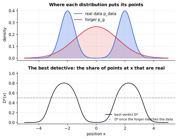
Reading it: the top panel shows two distributions on a line: the real data (blue) has two narrow bumps at −2 and +2, and the forger (red) spreads one wide bump over the middle. The bottom panel is the best verdict $D^$ at every position. Over the real bumps it rises to about 0.8, because most points found there are real (the forger's wide bump still reaches them). In the middle and at the far edges it falls towards 0, because only fakes live there. The grey dashed line at 0.5 is what $D^$ becomes once the forger matches the data: the detective has nothing left to go on. The shape of the bottom curve is exactly the information the forger needs, which way to move its mass.
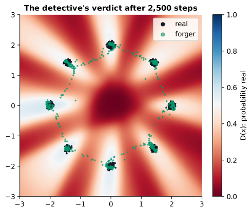
Reading it: this is the real ring after 2,500 rounds of training. The background colour is the trained detective's verdict at every spot: blue for "real", red for "fake", white for 0.5. Black dots are real points, green dots are the forger's. The green points sit on all eight clouds, and the background there is pale, close to white: at the eight centres the verdict is between 0.46 and 0.58. That is the equilibrium made visible, the detective reduced to guessing where the forgery is good. Away from the ring, where neither real nor fake points ever appear, the formula says nothing, and the detective's colouring there is arbitrary (deep red in the empty middle).
Why it matters: the detective never needs to model what real data looks like; it only estimates a ratio between two densities. That is why GANs could learn sharp images long before anyone could write down a probability for an image.
In code: optimal_discriminator is the formula, fit_discriminator_table trains the most flexible detective possible (one free score per point) against a fixed forger and arrives at the same verdicts without being told the formula, and detective_verdicts evaluates a trained detective anywhere on the page.
Why the forger uses a different loss
Everyday picture. Early in training, the forger is terrible and the detective is sure every fake is fake. Now picture a game of "hotter, colder" where the helper stops talking once you are far enough away: the further off you are, the quieter the hints. That is the original forger loss. The fix is a helper who shouts louder the further off you are.
Tiny worked example. The detective looks at a fake and is 99% sure it is fake: D(G(z)) = 0.01. How hard does each loss push the forger?
- The original loss, log(1 − D(G(z))), which the forger minimises: its slope with respect to the detective's score is −D = −0.01. Almost nothing.
- The non-saturating loss, −log D(G(z)), which the forger also minimises: its slope is −(1 − D) = −0.99. Ninety-nine times more.
When the detective is undecided, D = 0.5, both slopes are −0.5. The two losses agree when it doesn't matter and differ exactly when it does.
Level 3: the formula and its symbols
$$ \frac{\partial}{\partial a}\,\log\big(1 - \sigma(a)\big) = -\sigma(a) = -D \qquad\qquad \frac{\partial}{\partial a}\,\big(-\log \sigma(a)\big) = -\big(1 - \sigma(a)\big) = -(1 - D) $$
Symbols
| Symbol | Meaning here | In the example |
|---|---|---|
| $a$ | the detective's score for a fake, before the sigmoid | $\log(0.01/0.99) = -4.6$ |
| $\sigma(a)$ | the verdict D on that fake | 0.01 |
| $\frac{\partial}{\partial a}$ | the derivative with respect to $a$: how much the loss changes when the score is nudged up a tiny amount (see primer.notation) |
|
| $\log(1 - \sigma(a))$ | the original, "saturating" forger loss | $\log 0.99$ |
| $-\log \sigma(a)$ | the non-saturating forger loss | $-\log 0.01 = 4.6$ |
In words: "the original loss changes by only D when the detective's score moves, so it goes quiet when D is near 0; the non-saturating loss changes by 1 − D, so it is loudest exactly when the forger is doing worst."
With the numbers: at D = 0.01, the slopes are −0.01 and −0.99.
Level 3: in Python
In Python:
import math
def sigma(a):
    return 1 / (1 + math.exp(-a))
# a score that makes the detective 99% sure the fake is fake
a = math.log(0.01 / 0.99)
round(sigma(a), 2)  # → 0.01
# measure each slope by nudging the score a tiny bit either way
h = 1e-6
def slope(loss):
    return (loss(a + h) - loss(a - h)) / (2 * h)
def saturating(a):
    return math.log(1 - sigma(a))
def non_saturating(a):
    return -math.log(sigma(a))
round(slope(saturating), 3)  # → -0.01
round(slope(non_saturating), 3)  # → -0.99
Both losses want the same thing, a higher verdict on the fakes, and they share the same equilibrium. Only the strength of the push differs. The original GAN paper already recommended the switch, and essentially every GAN since uses the non-saturating loss or a Wasserstein-style loss (below).
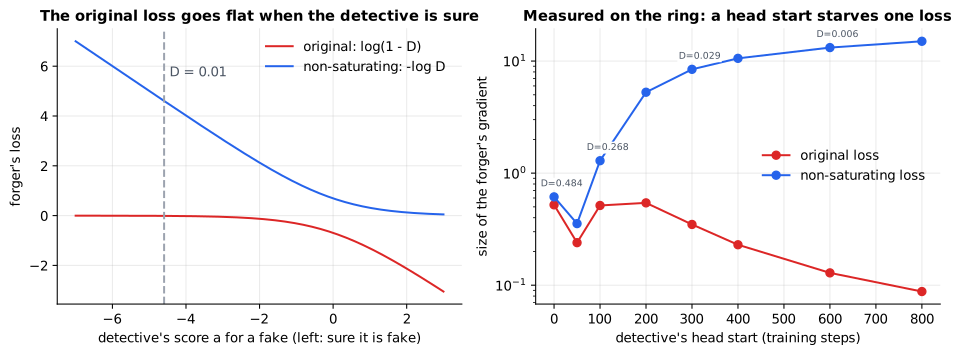
Reading it: on the left, the x-axis is the detective's score for a fake: far left means "certainly fake". The red curve, the original loss, goes flat as you move left, and a flat curve has no slope, so no gradient. The blue curve, the non-saturating loss, keeps a steady downhill slope all the way. On the right is a measurement from our ring: the detective trains alone against a frozen, untrained forger for more and more steps, and we measure how big a gradient each loss would hand the forger (log scale). At the start both are about 0.5 to 0.6. After 800 detective steps its verdict on fakes is 0.003, the original loss's gradient has shrunk to 0.09, and the non-saturating one has grown to 15: over a hundred times larger.
Why it matters: a forger that gets no gradient does not learn, and the detective's lead only widens. Early in training the detective always has the easy job, so this failure is the default, not an edge case.
In code: generator_logit_gradient returns both slopes, and head_start_experiment gives the detective a head start and measures the forger's gradient under each loss.
Why training is unstable, part 1: the players chase each other in circles
Everyday picture. Two people share an office thermostat. One turns the heat up whenever it feels cold; the other opens a window whenever it feels hot. Each reacts to where the room was, so the temperature overshoots one way, then the other, and never settles. A GAN's players do the same: the forger moves to where the detective currently says "real", and by the time it arrives, the detective has moved.
Tiny worked example. The smallest GAN there is, the Dirac GAN, has one number per player. The real data is a single point at x = 0. The forger has one number θ and always outputs x = θ. The detective has one number ψ and scores a point as ψ · x, so D(x) = σ(ψx). Start with the forger at θ = 1 and a detective with ψ = 0 (it cannot tell anything apart), and let both take steps of size 1 at the same time:
| Step | σ(ψθ) | θ (forger) | ψ (detective) | Distance from (0, 0) |
|---|---|---|---|---|
| 0 | 1 | 0 | 1 | |
| 1 | σ(0) = 0.5 | 1 | −0.5 | 1.118 |
| 2 | σ(−0.5) = 0.3775 | 0.811 | −0.878 | 1.195 |
After step 1 the detective has learned "bigger x means fake" (ψ turned negative), and after step 2 the forger has moved towards the data at 0. Both moves were sensible, yet the pair got further from the equilibrium, the point (0, 0) where the forger sits on the data and the detective is indifferent.
Level 3: the formula and its symbols
$$ V(\theta, \psi) = \log \sigma(\psi \cdot 0) + \log\big(1 - \sigma(\psi\theta)\big) \qquad \frac{\partial V}{\partial \psi} = -\sigma(\psi\theta)\,\theta \qquad \frac{\partial V}{\partial \theta} = -\sigma(\psi\theta)\,\psi $$
Symbols
| Symbol | Meaning here | In the example |
|---|---|---|
| $\theta$ | the forger's only number: where it puts its fake | 1 |
| $\psi$ | the detective's only number: the slope of its score $\psi x$ | 0 |
| $\psi \cdot 0$ | the detective's score for the real data at $x = 0$: always 0, so $D(0) = 0.5$ | 0 |
| $\sigma(\psi\theta)$ | the verdict on the fake | 0.5 |
| $\frac{\partial V}{\partial \psi}$ | the slope the detective climbs: $\psi \leftarrow \psi + \eta\,\frac{\partial V}{\partial \psi}$ | $-0.5$ |
| $\frac{\partial V}{\partial \theta}$ | the slope the forger descends: $\theta \leftarrow \theta - \eta\,\frac{\partial V}{\partial \theta}$ | 0 |
| $\eta$ | the step size (learning rate) | 1 |
| $\leftarrow$ | "is replaced by" |
In words: "the detective tilts its slope against wherever the fake sits; the forger slides along whichever way the slope says is more real; each reacts to the other's old position."
With the numbers: step 1: σ(0) = 0.5, so ψ becomes 0 − 1 · 0.5 · 1 = −0.5 and θ stays 1 + 1 · 0.5 · 0 = 1. Step 2: σ(−0.5) = 0.3775, so θ becomes 1 + 0.3775 · (−0.5) = 0.811 and ψ becomes −0.5 − 0.3775 · 1 = −0.878.
Level 3: in Python
In Python:
import math
def sigma(a):
    return 1 / (1 + math.exp(-a))
theta, psi, lr = 1.0, 0.0, 1.0
s = sigma(psi * theta)
s  # → 0.5
# both move at once, each using the other's old position
theta, psi = theta + lr * s * psi, psi - lr * s * theta
(theta, psi)  # → (1.0, -0.5)
s = sigma(psi * theta)
round(s, 4)  # → 0.3775
theta, psi = theta + lr * s * psi, psi - lr * s * theta
(round(theta, 3), round(psi, 3))  # → (0.811, -0.878)
# distance from the equilibrium (0, 0): 1, then 1.118, then 1.195
round(math.hypot(theta, psi), 3)  # → 1.195
flowchart LR
  A["fake sits to the right<br/>of the data"] --> B["detective tilts:<br/>right means fake"]
  B --> C["forger slides left,<br/>overshoots past the data"]
  C --> D["detective tilts back:<br/>left means fake"]
  D --> E["forger slides right,<br/>overshoots again"]
  E --> A
Reading it: the boxes form a loop because the game has no downhill direction that both players share. Each arrow is a sensible move for the player making it, but each player only reacts to the other's current position, so the forger arrives just after the detective has changed its mind. The loop is a rotation around the equilibrium, not a descent into it.
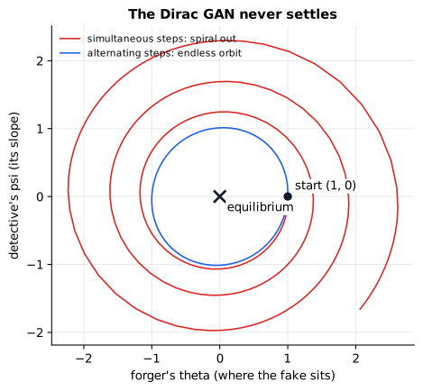
Reading it: the horizontal axis is the forger's θ, the vertical axis the detective's ψ, and the black cross at (0, 0) is the equilibrium. Both paths start at the dot, (1, 0), and take 300 steps of size 0.2. The red path, where both players step at once, spirals outwards: after 300 steps it is 2.6 away from the equilibrium, where it started 1 away. The blue path, where the forger waits to see the detective's new ψ before it moves, stays on a closed loop about 1 away forever. Neither ever arrives. Plain gradient steps do not solve this game even in two dimensions.
Why it matters: a real GAN has millions of numbers per player, and this rotation happens in many directions at once. It shows up as losses that swing up and down without trending, and samples that keep changing character instead of steadily improving.
In code: dirac_gan runs this two-number game with simultaneous or alternating steps.
Why training is unstable, part 2: mode collapse
Everyday picture. The forger discovers that one particular note, say the twenty, always fools the detective. So it prints nothing but twenties. The detective eventually learns that twenties are suspicious, so the forger switches to printing only fifties, and so on. Each forgery is good, but the forger never produces the full variety of real money. Each distinct kind of real example is a mode, and settling on a few of them is mode collapse.
Tiny worked example. To measure variety on the ring, generate 1,000 points and count, for each of the eight clouds, how many land within 0.15 of its centre (3 spreads). A cloud is covered if it gets at least 20 of the 1,000 (2%; a perfect forger gives each about 125). A point that lands near any centre counts as high quality. After 2,500 rounds with equal learning rates for both players, the counts for the eight clouds are (0, 68, 0, 20, 0, 51, 0, 17). Clouds 2, 4 and 6 are covered, cloud 8's 17 falls short, so 3 of 8 modes are covered, and only 156 of the 1,000 points are high quality: the rest are strung between clouds.
stateDiagram-v2
  direction LR
  EvenClouds: forger piles onto clouds 1, 3, 5, 7
  CatchEven: detective learns those clouds are suspicious
  OddClouds: forger jumps to clouds 2, 4, 6, 8
  CatchOdd: detective learns these are suspicious
  EvenClouds --> CatchEven
  CatchEven --> OddClouds
  OddClouds --> CatchOdd
  CatchOdd --> EvenClouds
Reading it: each box is a phase of training, and the arrows go round in a circle. The forger does not have to cover every cloud to fool the detective today; it only has to put its points where the detective currently says "real". The detective then learns those spots are over-supplied with fakes, the verdict there drops, and the forger's gradient pushes the whole pile somewhere else. It is the chase from part 1, now played out across the clouds of the data. The alternation between odd and even clouds is what our run actually does, pictured next.
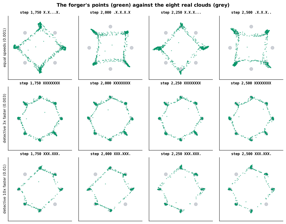
Reading it: each panel is the page, grey circles mark the eight real clouds, and green dots are 1,000 points from the forger at that step (always made from the same noise, so the panels are comparable). The panel titles spell the coverage with X for a covered cloud, counting anticlockwise from the cloud on the right. Top row, equal learning rates: the green points hop from clouds 1, 3 and 7 at step 1,750 to 2, 4, 6 and 8 at step 2,000, back to 1, 3 and 5, then to 2, 4 and 6, never holding more than half the ring. Middle row, a detective that learns three times faster than the forger: all eight clouds, every snapshot. Bottom row, a detective ten times faster: six clouds, and the same six at every snapshot. Two clouds stay empty for good.
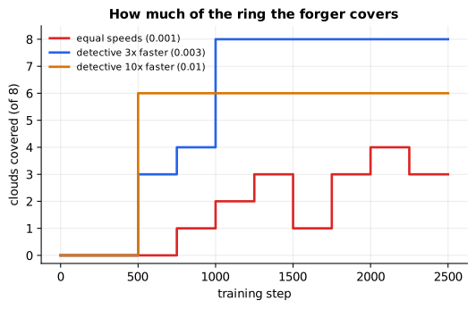
Reading it: the x-axis is the training step, the y-axis the number of clouds covered out of eight. The blue line (detective three times faster) climbs to 8 by step 1,000 and stays there. The red line (equal speeds) zigzags between 1 and 4, the hopping from the top row above. The amber line (detective ten times faster) jumps to 6 by step 500 and never moves again. The same code and the same data give three very different outcomes, and the only thing that changed is how fast the detective learns.
These runs use one fixed seed. With other seeds the equal-speed run sometimes finds all eight clouds late on, and the ten-times run sometimes escapes after a while; the pattern, not the exact counts, is the lesson.
Why it matters: mode collapse is the classic GAN failure on real data. A face generator that has collapsed produces beautiful faces that all look like the same few people. Quality metrics that look at one sample at a time can't see it; you have to measure coverage, as we did here.
In code: mode_coverage counts covered clouds and high-quality points, and train_gan records it every 250 steps.
Why training is unstable, part 3: a detective that wins too fast
Everyday picture. A detective who learns much faster than the forger soon rejects everything outside the few spots the forger has already mastered, with total confidence. Every small experiment the forger tries in a new direction comes back "more fake", so it retreats to what already works and stops exploring.
Tiny worked example. The bottom row above: with the detective's learning rate ten times the forger's, after 2,500 steps the counts per cloud are (199, 181, 117, 0, 132, 160, 72, 0). The six covered clouds are served well: 86% of points are high quality, more than the balanced run's 81%. But clouds 4 and 8 get nothing, from step 500 until the end. Better-looking samples, less variety: a trade-off you will meet again with real image generators.
flowchart LR
  A["detective learns<br/>much faster"] --> B["gaps between the forger's clouds<br/>become confident fake zones"]
  B --> C["every small step towards them<br/>lowers the verdict"]
  C --> D["forger polishes the clouds<br/>it already has"]
  D --> E["empty clouds stay empty"]
Reading it: read it as a chain of causes. A fast detective turns every region the forger isn't already covering into a wall of confident "fake" verdicts. To reach an empty cloud the forger would have to move points through such a wall. But a gradient only sees the next small step, and every small step into the wall makes the verdict worse, so the gradient pushes the points back onto the clouds they already occupy. The forger spends its effort sharpening those, and the missing ones are never discovered.
Why it matters: "just train the detective harder" sounds like it should give the forger a better teacher. Past a point it gives it a worse one. The detective needs to be good enough to point the way, not so good that it only says no.
In code: train_gan takes both learning rates as arguments; this run gives the detective ten times the forger's.
Fixes that make the game trainable
Everyday picture. A good sparring partner matters more than a strong one. Every stabiliser below is a way of keeping the detective useful: fast enough to teach, smooth enough that its verdicts point somewhere.
flowchart LR
  P1["players out of step"] --> F1["careful learning rates<br/>two time-scales"]
  P2["detective builds<br/>steep cliffs"] --> F2["gradient penalty"]
  P2 --> F3["spectral normalization"]
  P3["piles don't overlap,<br/>so the verdict gives no direction"] --> F4["Wasserstein distance"]
  F4 --> F2
Reading it: failures are on the left and the fixes that target them on the right. Players moving out of step are fixed by choosing their speeds. A detective whose verdict jumps from 0 to 1 across a narrow cliff is fixed by penalising or capping its steepness. A yardstick that can't tell "near miss" from "far miss" is replaced by the Wasserstein distance, which in practice needs one of the steepness fixes to compute, hence the last arrow.
Careful learning rates
Everyday picture. Pace the two sparring partners so that neither runs away with the match.
Tiny worked example. The three rows of the ring figure differ only in the detective's learning rate, with the forger's fixed at 0.001:
| Detective's rate | Clouds covered at step 2,500 | High-quality points |
|---|---|---|
| 0.001 (equal) | 3, and hopping | 16% |
| 0.003 (three times) | 8, steady | 81% |
| 0.01 (ten times) | 6, stuck | 86% |
A modestly faster detective keeps its verdicts close to the best-detective formula for the forger it is facing now, so the forger follows a gradient that points at the data rather than at yesterday's detective. Heusel and colleagues called this the two time-scale update rule and proved it reaches an equilibrium under reasonable conditions. The right ratio depends on the problem; the lesson is that it is a dial worth turning.
In code: train_gan with a detective learning rate of 0.003 is the balanced run; the other two rows are the same call with 0.001 and 0.01.
Gradient penalty: fine the detective for steep cliffs
Everyday picture. Charge the detective a fee for how sharply its score changes right on top of the real data. A detective with gentle slopes still ranks real above fake, but it can no longer swing wildly, and the swinging is what fed the spiral in part 1.
Tiny worked example. In the Dirac GAN the detective's score is ψ · x, whose slope with respect to x is just ψ. The R1 gradient penalty adds (γ / 2) · ψ² to what the detective minimises. With γ = 1 and ψ = −0.5 the fee is 0.125, and its gradient, γψ = −0.5, pulls ψ back towards 0 on every step, like friction. With step size 0.2 that friction shrinks ψ by a factor 1 − 0.2 · 1 = 0.8 per step, on top of the game's own push.
Level 3: the formula and its symbols
$$ R_1 = \frac{\gamma}{2}\;\mathbb{E}_{x \sim p_{\text{data}}}\Big[\big\lVert \nabla_x\, a(x) \big\rVert^2\Big] $$
Symbols
| Symbol | Meaning here | In the Dirac example |
|---|---|---|
| $R_1$ | the penalty added to the detective's loss | 0.125 |
| $\gamma$ | how heavily steepness is fined | 1 |
| $a(x)$ | the detective's score at $x$ | $\psi x$ |
| $\nabla_x\, a(x)$ | the gradient of the score with respect to the input point: which way, and how steeply, the score rises as you move $x$ | $\psi = -0.5$ |
| $\lVert \cdot \rVert^2$ | the squared length of that gradient (see primer.notation, the length of a vector) |
0.25 |
| $\mathbb{E}_{x \sim p_{\text{data}}}$ | averaged over real points only | the single real point $x = 0$ |
In words: "measure how steeply the detective's score changes at the real points, square it, average it, and charge the detective γ/2 times that."
With the numbers: (1 / 2) · (−0.5)² = 0.125.
Level 3: in Python
In Python:
gamma, psi = 1.0, -0.5
# slope of the score psi * x with respect to x, at the real point
slope = psi
gamma / 2 * slope ** 2  # → 0.125
# the penalty's pull on psi: its derivative, gamma * psi
gamma * psi  # → -0.5
# one step of size 0.2 against that pull shrinks psi by a factor 0.8
round(psi - 0.2 * gamma * psi, 2)  # → -0.4
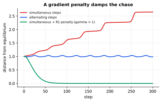
Reading it: the x-axis is the step, the y-axis the distance of (θ, ψ) from the equilibrium (0, 0). The red line (plain simultaneous steps) climbs in steps, one per lap: the outward spiral. The blue line (alternating steps) hovers near 1 forever: the endless orbit. The green line adds the R1 penalty with γ = 1 to the simultaneous steps and dives: 0.08 after 50 steps, essentially 0 by
- The friction turns the rotation into a spiral inwards. That is the Mescheder, Geiger and Nowozin result in two numbers, and it is why StyleGAN and many later GANs train with an R1 penalty. The Wasserstein GAN with gradient penalty (WGAN-GP) uses the same idea with a different target: it keeps the slope near 1 at points between real and fake.
In code: dirac_gan takes the penalty weight γ as an argument and adds the R1 penalty's pull, −γψ, to the detective's step.
Wasserstein distance: a yardstick that knows near from far
Everyday picture. Picture the real data and the fakes as two piles of sand. The Wasserstein distance, also called the earth mover's distance, is the least work needed to reshape one pile into the other: the amount of sand moved times how far it travels. The Jensen-Shannon divergence from the best-detective section only asks how much the piles overlap.
Tiny worked example. Put all the real sand at x = 0 and all the fake sand at x = θ. If θ = 1, the piles don't overlap, and the Jensen-Shannon divergence is log 2 = 0.693. If θ = 5, they still don't overlap, and it is still 0.693. It cannot tell a near miss from a far one, so it gives the forger no direction. The Wasserstein distance is 1 for θ = 1 and 5 for θ = 5: it shrinks as the forger approaches, so it always points home.
For two equally sized samples on a line, the cheapest way to move the sand is to pair the smallest with the smallest, the next with the next, and so on:
Level 3: the formula and its symbols
$$ W_1 = \frac{1}{n} \sum_{i=1}^{n} \big\lvert a_{(i)} - b_{(i)} \big\rvert $$
Symbols
| Symbol | Meaning here | In the example |
|---|---|---|
| $W_1$ | the Wasserstein (earth mover's) distance between two piles on a line | 3 |
| $n$ | how many grains (samples) each pile has | 3 |
| $a_{(i)}$ | the $i$-th smallest value in the first pile (the brackets mean "after sorting") | $a = (0, 1, 2)$ |
| $b_{(i)}$ | the $i$-th smallest value in the second pile | $b = (5, 3, 4)$ sorts to $(3, 4, 5)$ |
| $\lvert \cdot \rvert$ | the absolute value: the gap, ignoring direction | $\lvert 0 - 3 \rvert = 3$ |
In words: "sort both piles, pair them up in order, and average how far each grain has to travel."
With the numbers: pairs (0, 3), (1, 4), (2, 5), gaps 3, 3, 3, average 3.
Level 3: in Python
In Python:
a = [0, 1, 2]
b = [5, 3, 4]
# pair the smallest with the smallest, and so on
pairs = list(zip(sorted(a), sorted(b)))
pairs  # → [(0, 3), (1, 4), (2, 5)]
sum(abs(x - y) for x, y in pairs) / len(pairs)  # → 3.0
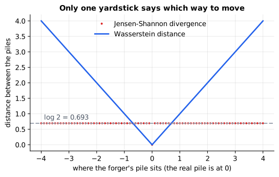
Reading it: the x-axis is where the forger's pile sits; the real pile is at 0. The red line (Jensen-Shannon) is flat at 0.693 everywhere except the single point θ = 0, where it drops to 0: a flat line has no slope, so nothing tells the forger which way to move. The blue V (Wasserstein) slopes down towards 0 from both sides: wherever the forger is, the slope points at the data. On images, where real photos and early fakes barely overlap, this difference is the difference between learning and not.
The Wasserstein GAN replaces the detective with a critic that outputs an unbounded score instead of a probability, and trains it so that the gap between its average score on real and on fake points estimates this distance. The catch: the estimate is only valid if the critic's slope is at most 1 everywhere. The original WGAN enforced that crudely by clipping every weight; WGAN-GP does it with a gradient penalty; spectral normalization, next, does it by capping each layer.
In code: wasserstein_1d is the sort-and-pair formula, and js_divergence computes the Jensen-Shannon divergence between two histograms, flat at log 2 whenever they don't overlap.
Spectral normalization: a speed limit on every layer
Everyday picture. A layer of a network is a matrix, and a matrix stretches some directions more than others. If no layer can stretch anything by more than 1, the whole detective can't change its score faster than the input changes: its cliffs have a speed limit.
Tiny worked example. The matrix W = [[3, 0], [0, 1]] stretches the horizontal direction by 3 and the vertical by 1. Its largest stretch is
- Divide W by 3 and no direction is stretched by more than 1.
Level 3: the formula and its symbols
$$ \bar W = \frac{W}{\lVert W \rVert_2} \qquad \lVert W \rVert_2 = \max_{\lVert v \rVert = 1} \lVert W v \rVert $$
Symbols
| Symbol | Meaning here | In the example |
|---|---|---|
| $W$ | one layer's weight matrix (see primer.notation for matrices) |
[[3, 0], [0, 1]] |
| $v$ | an input direction: an arrow of length 1 | $(1, 0)$ |
| $\lVert v \rVert$ | the length of $v$ | 1 |
| $Wv$ | the arrow after passing through the layer | $(3, 0)$ |
| $\max_{\lVert v \rVert = 1}$ | "the largest value over every arrow of length 1" | |
| $\lVert W \rVert_2$ | the spectral norm: the most W lengthens any arrow | 3 |
| $\bar W$ | the normalised layer used in the detective | [[1, 0], [0, 1/3]] |
In words: "find the direction the layer stretches most, and divide the whole layer by that stretch."
With the numbers: $(1, 0)$ becomes $(3, 0)$, length 3; $(0, 1)$ stays length 1; every other direction lands in between. So $\lVert W \rVert_2 = 3$, and $W / 3$ stretches by at most 1.
Level 3: in Python
In Python:
import math
W = [[3, 0], [0, 1]]
def stretch(v):
    Wv = [sum(w * x for w, x in zip(row, v)) for row in W]
    return math.hypot(*Wv) / math.hypot(*v)
# try unit arrows all the way round the circle, one per degree
angles = [2 * math.pi * k / 360 for k in range(360)]
round(max(stretch((math.cos(t), math.sin(t))) for t in angles), 3)  # → 3.0
# divide W by its largest stretch
W = [[w / 3 for w in row] for row in W]
round(max(stretch((math.cos(t), math.sin(t))) for t in angles), 3)  # → 1.0
Trying every direction is fine for a 2 × 2 matrix but not for a layer with a thousand inputs. Power iteration finds the most-stretched direction cheaply:
flowchart LR
  V["start: any arrow v"] --> U["u = W v,<br/>rescaled to length 1"]
  U --> B["v = W transpose u,<br/>rescaled to length 1"]
  B --> Q{"repeat"}
  Q -- again --> U
  Q -- done --> S["largest stretch = length of W v"]
Reading it: push an arrow through the layer and back through its transpose, over and over. Each round trip multiplies the arrow's most-stretched component by more than any other, so the arrow swings round to point along that direction, and the stretch is read off at the end. Spectral normalization keeps one arrow per layer and runs a single round trip per training step: the weights change slowly, so the arrow stays nearly right, and the cost is a couple of extra matrix-vector products.
Why it matters: spectral normalization (Miyato and colleagues, 2018) is a one-line change to the detective that made GAN training far less sensitive to learning rates and architecture, and it became a default in large image GANs such as BigGAN.
In code: largest_stretch is power iteration, and spectrally_normalize divides a matrix by it.
Where GANs stand today
Everyday picture. The forger-and-detective idea started as the whole machine. Today it is more often a picky critic inside another machine, brought in for the one thing it does best: making outputs look sharp and real.
Tiny worked example. A GAN makes an image in one pass through the
generator. A diffusion model typically runs its network tens of times per
image, removing a little noise each time (see
primer.ml.generative.diffusion). For a while, that speed plus very sharp
samples (StyleGAN's faces, from 2018, are still striking) made GANs the best
image generators. Then diffusion models overtook them on image quality and,
above all, on coverage: they don't mode-collapse and they train stably,
which is everything this lesson has been fighting. Since around 2021 most
new image and video generators are diffusion or flow models.
GANs didn't disappear. Their loss did the moving:
flowchart LR
  X["real image or audio"] --> E["encoder"]
  E --> C["compact code"]
  C --> DEC["decoder"]
  DEC --> Y["reconstruction"]
  Y --> L1["reconstruction loss<br/>pixel or perceptual"]
  X --> L1
  Y --> DISC["detective:<br/>real or reconstructed?"]
  X --> DISC
  L1 --> T["total loss for<br/>encoder and decoder"]
  DISC --> T
Reading it: this is an autoencoder (see
primer.ml.generative.autoencoders) with a detective bolted on. The top
path squeezes the input into a compact code and rebuilds it. A
reconstruction loss alone rewards averages, and the average of many
plausible textures is a blur. The detective on the lower path looks at the
reconstruction and the original and asks "which is real?", which punishes
blur and rewards crisp detail. The decoder is trained on both losses
together. This design is how the image autoencoders inside latent diffusion
models are trained, how VQGAN's image tokenizer is trained, and how neural
audio decoders such as HiFi-GAN produce clean waveforms. GAN-style losses
are also used to distil a slow many-step diffusion model into a fast one-
or few-step generator.
Why it matters: when you meet a modern image, audio or video system, expect a GAN loss somewhere in its decoder or its fast sampling path, even when the headline method is diffusion. Everything in this lesson, the non-saturating loss, gradient penalties, spectral normalization and careful learning rates, is still how those critics are kept stable.
In 20 seconds
- A GAN trains a generator (forger) to turn noise into samples and a discriminator (detective) to tell real samples from fakes, against each other. The forger learns only through the detective's gradient.
- The game: min over G of max over D of E[log D(x)] + E[log(1 − D(G(z)))]. The best detective says p_data / (p_data + p_g); at the equilibrium the forger matches the data and the detective says 1/2 everywhere.
- The non-saturating loss (maximise log D(G(z))) keeps the forger's gradient strong when the detective is confident, exactly when the original loss goes quiet.
- Unstable because each player's target moves: plain gradient steps circle or spiral around the equilibrium, the forger hops between a few modes (mode collapse), and a detective that wins too fast freezes it.
- Fixes: balanced learning rates, gradient penalties (R1, WGAN-GP), spectral normalization, and the Wasserstein distance, which still points the way when real and fake don't overlap.
- Today: diffusion has overtaken GANs for generating images, but adversarial losses remain inside image and audio decoders and fast distilled samplers.
Self-test questions
Explain a GAN to a non-engineer in 30 seconds. Two programs play a game. One makes fake pictures; the other looks at real and fake pictures and guesses which is which. Every time the guesser catches a fake, the faker learns what gave it away and improves. After enough rounds the fakes are good enough that the guesser is reduced to guessing, and the faker has learned to make realistic pictures without anyone ever describing what a picture should look like.
Why does the generator never need to see real data? It learns only from the discriminator's gradient with respect to its own outputs: which way to move each fake so the discriminator finds it more real. The discriminator has seen real data, so its verdicts carry that information to the generator.
What does the optimal discriminator compute, and what does it say at equilibrium? D*(x) = p_data(x) / (p_data(x) + p_g(x)): the share of points found at x that are real. When the generator matches the data, p_g = p_data and D* is 1/2 everywhere, the value is −log 4, and the discriminator can do no better than a coin flip.
Why do almost all GANs use the non-saturating generator loss? The original loss log(1 − D(G(z))) has a slope of −D with respect to the discriminator's score, which is near zero when the discriminator confidently rejects fakes, as it does early in training. The non-saturating loss −log D(G(z)) has slope −(1 − D), largest exactly then. Both have the same equilibrium.
What is mode collapse, and how would you detect it? The generator covers only some of the distinct kinds of data (modes), often hopping between them as the discriminator catches up. Per-sample quality can look excellent, so you detect it by measuring coverage: how many modes or classes receive samples, or a distribution-level metric such as FID on real data.
Why doesn't plain gradient descent find the GAN equilibrium? The game has no shared downhill direction. Near the equilibrium the two players' updates form a rotation, so simultaneous steps spiral outward and alternating steps orbit forever, as the two-number Dirac GAN shows. Damping the discriminator with a gradient penalty turns the spiral inward.
Why is the Wasserstein distance a better training signal than Jensen-Shannon divergence? When the real and generated distributions don't overlap, Jensen-Shannon is stuck at log 2 however far apart they are, so it gives no direction. Wasserstein measures how far the mass must move, so it shrinks steadily as the generator approaches the data. Estimating it needs a critic whose slope is capped, which is what weight clipping, gradient penalties and spectral normalization provide.
If diffusion models won, why learn GANs? Adversarial losses are still how many image and audio decoders get sharp output, and how some diffusion models are distilled into one-step generators. And the instabilities here, moving targets and collapsing variety, show up wherever two models are trained against each other.
The papers behind this lesson
- Goodfellow et al., Generative Adversarial Nets (2014): https://arxiv.org/abs/1406.2661. Introduced the generator-discriminator game, derived the optimal discriminator and the equilibrium where the generator matches the data, and suggested the non-saturating loss. Annotated companion
- Metz, Poole, Pfau and Sohl-Dickstein, Unrolled Generative Adversarial Networks (2016): https://arxiv.org/abs/1611.02163. Used the ring of eight Gaussians to show a generator hopping between modes, and reduced it by letting the generator look ahead at several discriminator steps.
- Heusel et al., GANs Trained by a Two Time-Scale Update Rule Converge to a Local Nash Equilibrium (2017): https://arxiv.org/abs/1706.08500. Showed that separate learning rates for the two players give provable convergence, and introduced the FID score for judging generated images.
- Arjovsky, Chintala and Bottou, Wasserstein GAN (2017): https://arxiv.org/abs/1701.07875. Replaced the Jensen-Shannon objective with the earth mover's distance, which still gives a direction when real and generated data don't overlap. Annotated companion
- Gulrajani et al., Improved Training of Wasserstein GANs (2017): https://arxiv.org/abs/1704.00028. Enforced the Wasserstein critic's slope limit with a gradient penalty instead of weight clipping.
- Mescheder, Geiger and Nowozin, Which Training Methods for GANs do actually Converge? (2018): https://arxiv.org/abs/1801.04406. Introduced the two-number Dirac GAN to show why plain GAN training circles instead of converging, and the R1 penalty that makes it converge.
- Miyato et al., Spectral Normalization for Generative Adversarial Networks (2018): https://arxiv.org/abs/1802.05957. Capped every discriminator layer's largest stretch at 1 using one step of power iteration per training step.
Further reading
- Goodfellow, NIPS 2016 Tutorial: Generative Adversarial Networks: https://arxiv.org/abs/1701.00160
- Radford, Metz and Chintala, Unsupervised Representation Learning with Deep Convolutional GANs (DCGAN, 2015): https://arxiv.org/abs/1511.06434
- Karras, Laine and Aila, A Style-Based Generator Architecture for Generative Adversarial Networks (StyleGAN, 2018): https://arxiv.org/abs/1812.04948
- Dhariwal and Nichol, Diffusion Models Beat GANs on Image Synthesis (2021): https://arxiv.org/abs/2105.05233
- Esser, Rombach and Ommer, Taming Transformers for High-Resolution Image Synthesis (VQGAN, 2020): https://arxiv.org/abs/2012.09841
- Rombach et al., High-Resolution Image Synthesis with Latent Diffusion Models (2021): https://arxiv.org/abs/2112.10752
- Kong, Kim and Bae, HiFi-GAN: Generative Adversarial Networks for Efficient and High Fidelity Speech Synthesis (2020): https://arxiv.org/abs/2010.05646
- Sauer et al., Adversarial Diffusion Distillation (2023): https://arxiv.org/abs/2311.17042
- PyTorch, DCGAN Tutorial: https://pytorch.org/tutorials/beginner/dcgan_faces_tutorial.html
1r""" 2# GANs: a forger against a detective 3 4Run: `python -m primer.ml.generative.gans` 5 6This lesson builds on the small networks and gradients of 7`primer.ml.neural_net`, the binary cross-entropy of `primer.ml.losses` and 8the Adam optimizer of `primer.ml.optimizers`; `primer.notation` explains 9every symbol from zero. 10 11## Level 1: The practitioner's guide 12 13**In one sentence.** A generative adversarial network (GAN) trains a 14generator to turn random noise into samples by pitting it against a 15discriminator that learns to tell its samples from real ones, which yields 16sharp output in a single pass at the price of a training game that is hard 17to keep stable. 18 19**When you need it.** Two tells. You need a generator that runs in one 20pass, because it sits in a real-time loop (a speech vocoder, an interactive 21tool, a game) and a many-step diffusion sampler is too slow. Or you have a 22decoder that rebuilds images or audio and its output is blurry: a 23reconstruction loss rewards averages, and an adversarial loss is the 24standard cure. You don't need to train a GAN from scratch to generate new 25images or video today: since 2021 diffusion and flow models are the default 26there, because they train stably and cover the data, which is exactly what 27this lesson shows GANs struggling to do. The number that shows the naive 28approach failing: on this lesson's toy data (eight small clouds on a ring), 29a GAN trained with the same learning rate for both players covers 3 of the 8 30clouds after 2,500 rounds, and only 16% of its samples land on any cloud. 31Change nothing but the discriminator's learning rate to three times the 32generator's and it covers all 8 with 81% on target. 33 34**Your options.** From the least commitment to the most: 35 36| Option | What it does | What it guarantees | What it costs | Where it lives | 37|---|---|---|---|---| 38| A diffusion or flow model instead | Generates by removing noise over many passes | Stable training, full coverage; matches BigGAN-deep's image quality with 25 passes and better coverage | Tens of network passes per sample | A hosted API or a diffusion library | 39| A pretrained GAN generator | One pass from noise to sample, with an editable latent space | Real-time generation in its domain (faces, one class of object) | You are limited to domains someone trained; less variety than diffusion | Released checkpoints (StyleGAN family) | 40| Train a GAN with the standard stabilisers | Non-saturating loss, a faster discriminator, an R1 penalty or spectral normalization | A one-pass generator for your own narrow domain | Two networks, coverage monitoring, learning-rate tuning; a run can still collapse | Your training loop | 41| Wasserstein critic (WGAN-GP) | Replaces the verdict with a distance that still points home when real and fake don't overlap | A gradient wherever the generator is, and a loss that tracks quality | Several critic steps per generator step, plus a gradient penalty | Your training loop | 42| Adversarial loss inside a decoder | A discriminator judges reconstructions against originals | Sharp detail where a reconstruction loss alone gives blur | One more network to train and keep stable | The training of VAEs, tokenizers and vocoders | 43| Adversarial distillation of a diffusion model | A student learns to match a diffusion teacher in 1 to 4 steps, with a discriminator keeping it sharp | Real-time sampling from a foundation model | A teacher, a distillation run, some loss of variety | The fast sampling path of a diffusion system | 44 45**How to choose.** Start from the latency you need and the variety you 46can't lose. 47 48- A new image, audio or video generator with no hard latency limit: use 49 diffusion or flow matching, and put adversarial losses only in the decoder 50 and in a distilled fast path. 51- One-pass generation is non-negotiable and the domain is narrow: a GAN 52 generator, trained with every stabiliser in the table, or a distilled 53 diffusion model if a teacher exists for your domain. 54- A blurry decoder: add a discriminator that compares reconstructions with 55 originals, and expect the same instabilities as any GAN. 56- A latent space to edit (age a face, change a pose): a style-based 57 generator, whose latent space was designed for disentangled control. 58- Whatever you pick, measure coverage, not just per-sample quality. Mode 59 collapse produces beautiful samples that all look the same, and a metric 60 that scores one sample at a time cannot see it. 61 62**What it costs.** Sampling is the GAN's strength: one generator pass per 63sample. HiFi-GAN generates 22.05 kHz speech 167.9 times faster than real 64time on one V100 GPU, and its small version runs 13.4 times faster than 65real time on a CPU; a diffusion model of the 2021 generation needed 25 66network passes per image to match BigGAN-deep. Training is where the cost 67lies: two networks, one loss surface that moves every time the other 68player steps, and a set of dials whose settings decide the outcome. On the 69ring, 2,500 rounds with the discriminator learning at 0.003 against the 70generator's 0.001 covers all eight clouds; at 0.001 it covers three and at 710.01 it covers six. Each stabiliser has a price. An R1 gradient penalty 72needs the gradient of the discriminator's own gradient, an extra backward 73pass on every discriminator step; spectral normalization costs a couple of 74matrix-vector products per layer per step; a Wasserstein critic is trained 75for several steps per generator step. Quality and variety trade against 76each other on every dial: the ten-times-faster discriminator gives 86% 77on-target samples against the balanced run's 81%, and leaves two clouds 78empty for good. BigGAN exposed the same trade as a knob, its truncation 79trick, which trades sample variety for fidelity. 80 81**What breaks.** 82 83- **Mode collapse.** The generator covers a few kinds of data and hops 84 between them as the discriminator catches up: on the ring, 3 clouds of 8, 85 alternating between odd and even ones every 250 steps. Track coverage 86 (FID or a per-class count) and rebalance the learning rates. 87- **A silent gradient.** With the original generator loss, a confident 88 discriminator hands the generator almost nothing: after an 800-step head 89 start its verdict on fakes is 0.003 and the gradient 0.09, against 15 with 90 the non-saturating loss. Use the non-saturating loss; every modern GAN 91 does. 92- **Oscillation.** Plain gradient steps rotate around the equilibrium 93 rather than descending into it: in the two-number Dirac GAN, simultaneous 94 steps drift from 1 away to 2.6 away in 300 steps. Losses that swing 95 without trending are the symptom; an R1 penalty (0.08 away after 50 96 steps) is the fix. 97- **A discriminator that wins too fast.** Every region the generator has 98 not reached becomes a wall of confident "fake", and the generator 99 polishes what it has: six clouds from step 500 to the end, at ten times 100 the generator's rate. A faster discriminator helps up to a point, then 101 hurts. 102- **No overlap, no direction.** When real and generated data don't overlap, 103 the original objective is flat (Jensen-Shannon stuck at 0.693 whether the 104 generator is 1 or 10 away). The Wasserstein critic's distance still 105 slopes towards the data. 106- **A seed that lies.** The same settings can find all eight clouds with one 107 seed and three with another. Judge a recipe over several seeds. 108 109**In the wild.** StyleGAN (Karras, Laine and Aila) is the reference 110one-pass image generator: a style-based generator that disentangles 111high-level attributes from stochastic detail, trained on the FFHQ face 112dataset the paper introduced, and trained with the R1 penalty. 113BigGAN scaled class-conditional GANs to ImageNet with spectral 114normalization, reaching an Inception Score of 166.5 and an FID of 7.4 at 115128 × 128. FID itself, the standard score for generated images, came from 116the two time-scale paper (Heusel et al.), along with the proof that 117separate learning rates converge. Dhariwal and Nichol's *Diffusion Models 118Beat GANs* marked the handover on image quality. Adversarial losses now 119live inside other systems: the autoencoders of latent diffusion and 120VQGAN's tokenizer are trained with a discriminator, HiFi-GAN and the neural 121audio codecs use adversaries to keep waveforms clean, and Adversarial 122Diffusion Distillation turns a diffusion model into a one-to-four-step 123sampler by pairing score distillation with an adversarial loss. Every paper 124is linked at the end of the lesson. 125 126**Go deeper.** Level 2 builds both players in NumPy, derives the best 127possible discriminator and the game's equilibrium, shows why the original 128generator loss goes silent, then reproduces each failure on the ring (the 129Dirac GAN's spiral, mode collapse, the over-strong discriminator) and runs 130each fix. If you only needed to choose, you are done. 131 132## Level 2: How it works, from scratch 133 134A forger wants to print banknotes that pass as real. A detective wants to 135catch every fake. At first the forger is hopeless: smudged ink, the wrong 136colour, and the detective spots every note. But every time the detective 137rejects a note, the forger learns *what gave it away* and fixes that. Every 138time the forger improves, the detective has to look more closely. Neither 139is ever told what a real banknote should look like. They only push against 140each other, and both keep getting better. 141 142The contest ends when the forger's notes are so good that the detective can 143do no better than guess: "real" half the time, "fake" the other half. At 144that point the forger has learned to make banknotes, and nobody ever wrote 145down a rule for what a banknote is. 146 147That is a **generative adversarial network**, a **GAN**. The forger is a 148neural network called the **generator**; the detective is a second network 149called the **discriminator**. Train them against each other on photos of 150faces and the generator learns to produce new faces that never existed. 151 152This lesson builds both players from scratch in NumPy, trains them on a toy 153picture you can see at a glance, and then shows the three ways the contest 154goes wrong: the players chase each other in circles, the forger settles for 155copying a few examples (**mode collapse**), and the detective wins so 156completely that the forger stops learning. Each failure gets a fix you can 157run. The same goal, making new samples, is reached differently by 158`primer.ml.generative.autoencoders` (squeeze and rebuild) and 159`primer.ml.generative.diffusion` (remove noise a little at a time). 160 161## The two players 162 163**Everyday picture.** The forger is a recipe that turns a few dice rolls 164into a banknote: different rolls, a different note. The detective is a 165machine you feed a note into, and out comes a single number, how sure it is 166that the note is real. 167 168**Tiny worked example.** Our "banknotes" are points on a flat page. The real 169data is a **ring of eight little clouds**: eight centres evenly spaced on a 170circle of radius 2, each real point scattered a tiny amount (a spread of 1710.05) around one centre, chosen at random. This toy picture comes from the 172research literature on GAN failures because you can *see* whether a forger 173has found all eight clouds. 174 175- The **generator** G takes two random numbers z (the dice rolls, drawn from 176 a bell curve) and returns one point on the page. It is a small neural 177 network: 2 numbers in, two layers of 32 tanh units, 2 numbers out. 178- The **discriminator** D takes a point and returns a probability that it is 179 real. It is another small network: 2 numbers in, 64 tanh units, one 180 **score** out, then squashed into the range 0 to 1. 181 182The squashing is the **sigmoid**, the same one `primer.ml.neural_net` uses to 183turn a score into a probability: 184 185$$ 186D(x) = \sigma\big(a(x)\big) = \frac{1}{1 + e^{-a(x)}} 187$$ 188 189**Symbols** 190 191| Symbol | Meaning here | In the example | 192|---|---|---| 193| $x$ | a point on the page, real or forged | $(2, 0)$ | 194| $a(x)$ | the detective's raw **score** for $x$ (also called a **logit**): any number, large and positive for "surely real" | $a(x) = x_1 - 1$ | 195| $x_1$ | the first coordinate of $x$ | 2 | 196| $e$ | Euler's number, about 2.718 (see `primer.notation`) | | 197| $\sigma$ | the sigmoid: squashes any score into a probability between 0 and 1 | $\sigma(1) = 0.731$ | 198| $D(x)$ | the detective's verdict: the probability that $x$ is real | 0.731 | 199 200**In words:** "the detective computes a score for the point, and the sigmoid 201turns the score into a probability that the point is real." 202 203**With the numbers:** take a detective with a single neuron whose score is 204$a(x) = x_1 - 1$. The point $(2, 0)$, one of the eight real centres, scores 205$2 - 1 = 1$, and $\sigma(1) = 1 / (1 + e^{-1}) = 0.731$: probably real. The 206point $(0, 0)$ in the middle of the ring scores $-1$ and gets 207$\sigma(-1) = 0.269$: probably fake. 208 209**In Python:** 210 211```python 212import math 213def sigma(a): 214 return 1 / (1 + math.exp(-a)) 215# a one-neuron detective: score a(x) = x_1 - 1 216def a(x): 217 return x[0] - 1 218round(sigma(a((2, 0))), 3) # → 0.731 219round(sigma(a((0, 0))), 3) # → 0.269 220``` 221 222```mermaid 223flowchart LR 224 Z["noise z<br/>2 random numbers"] --> G["Generator G<br/>the forger"] 225 G --> F["fake point G(z)"] 226 R["real point x<br/>from the ring"] --> D["Discriminator D<br/>the detective"] 227 F --> D 228 D --> P["D(point)<br/>probability it is real"] 229 P -. "learns to call real real<br/>and fake fake" .-> D 230 P -. "learns to make D say real<br/>about its fakes" .-> G 231``` 232 233**Reading it:** start at the far left. Noise goes into the generator and 234comes out as a fake point. Real points come in from the data. Both kinds of 235point go through the same detective, which gives each one a probability. 236The two dotted arrows are the learning signals, and they pull in opposite 237directions: the detective adjusts itself to score real points high and fakes 238low, and the generator adjusts itself to make the detective score *its* 239points high. Notice that the generator never sees a real point. Everything 240it learns about the data arrives through the detective's verdicts. 241 242**Why it matters:** that last point is the whole trick. Nobody writes down 243what a face, a voice or a banknote is. The detective discovers what separates 244real from fake, and its gradient (the direction that would make it less 245sure a fake is fake; see `primer.ml.neural_net` for gradients) tells the 246forger how to improve. 247 248**In code:** `ring_of_gaussians` draws real points around `ring_modes`, `MLP` is both players (its `MLP.backward` also returns the gradient with respect to the input, the channel through which the forger learns), with shapes `GENERATOR_SIZES` and `DISCRIMINATOR_SIZES`, and `sigmoid` turns the detective's score into a probability. 249 250## The game: one number both players fight over 251 252**Everyday picture.** Picture a scoreboard. The detective earns points for 253confident, correct calls and loses points, heavily, for confident mistakes. 254The detective wants the score as high as possible. The forger wants it as 255low as possible. One number, two players pulling it in opposite directions: 256that is a **minimax** game. 257 258**Tiny worked example.** The detective looks at two real notes and two 259fakes. The score uses the **logarithm** (log): log 1 = 0, and the log of a 260small number is a large negative number, so a confident mistake costs far 261more than a hesitant one (see `primer.notation` for logs from scratch). 262 263| Note | Real? | Verdict D | What is scored | Value | 264|---|---|---|---|---| 265| 1 | real | 0.9 | log D = log 0.9 | −0.105 | 266| 2 | real | 0.8 | log D = log 0.8 | −0.223 | 267| 3 | fake | 0.2 | log (1 − D) = log 0.8 | −0.223 | 268| 4 | fake | 0.4 | log (1 − D) = log 0.6 | −0.511 | 269 270The average over the real notes is −0.164, over the fakes −0.367, and the 271total is **−0.53**. A perfect detective (1 on every real note, 0 on every 272fake) would score log 1 + log 1 = 0, the ceiling. A detective reduced to a 273coin flip (0.5 on everything) scores log 0.5 + log 0.5 = −1.386. 274 275$$ 276\min_G \, \max_D \; V(D, G) = \mathbb{E}_{x \sim p_{\text{data}}}\big[\log D(x)\big] + \mathbb{E}_{z \sim p_z}\big[\log\big(1 - D(G(z))\big)\big] 277$$ 278 279**Symbols** 280 281| Symbol | Meaning here | In the example | 282|---|---|---| 283| $V(D, G)$ | the **value**: the scoreboard number | −0.53 | 284| $\max_D$ | "the detective chooses its weights to make what follows as large as possible" | | 285| $\min_G$ | "the forger chooses its weights to make that best-case value as small as possible" | | 286| $\mathbb{E}$ | **expectation**: the average over many draws (see `primer.notation`, probability notation) | an average over 2 notes | 287| $x \sim p_{\text{data}}$ | "$x$ drawn from the real data" | notes 1 and 2 | 288| $z \sim p_z$ | "$z$ drawn from the noise the forger starts from" | the dice rolls behind notes 3 and 4 | 289| $D(x)$ | the verdict on a real point | 0.9, 0.8 | 290| $G(z)$ | a fake point made from noise $z$ | notes 3 and 4 | 291| $D(G(z))$ | the verdict on a fake | 0.2, 0.4 | 292| $\log$ | natural logarithm: 0 at 1, very negative near 0 | $\log 0.6 = -0.511$ | 293 294**In words:** "average the log of the verdicts on real points, add the 295average log of one minus the verdicts on fakes; the detective pushes this 296number up, the forger pushes it down." 297 298**With the numbers:** (log 0.9 + log 0.8) / 2 + (log 0.8 + log 0.6) / 2 = 299−0.164 + (−0.367) = −0.53. 300 301**In Python:** 302 303```python 304import math 305# D(x) on two real notes, D(G(z)) on two fakes 306d_real, d_fake = [0.9, 0.8], [0.2, 0.4] 307# E over real x of log D(x): an average 308real_term = sum(math.log(d) for d in d_real) / len(d_real) 309round(real_term, 3) # → -0.164 310# E over noise z of log(1 - D(G(z))) 311fake_term = sum(math.log(1 - d) for d in d_fake) / len(d_fake) 312round(fake_term, 3) # → -0.367 313round(real_term + fake_term, 2) # → -0.53 314# a coin-flip detective, D = 1/2 on everything 315round(math.log(0.5) + math.log(0.5), 3) # → -1.386 316``` 317 318If this looks familiar, it should: −V is exactly the **binary 319cross-entropy** of a classifier that labels real points 1 and fakes 0 (see 320`primer.ml.losses`). The detective is an ordinary classifier. What is new 321is that its second class, the fakes, keeps changing underneath it. 322 323Training alternates. Nobody can solve "min over G of max over D" directly, 324so each round takes one small step for each player: 325 326```mermaid 327flowchart TB 328 S["sample a batch of real points<br/>and a batch of noise"] --> F["forger makes fakes G(z)"] 329 F --> DS["detective step:<br/>climb V, so D(real) rises<br/>and D(fake) falls"] 330 DS --> GS["forger step:<br/>change G so the new detective<br/>scores its fakes higher"] 331 GS --> CHK{"trained enough?"} 332 CHK -- no --> S 333 CHK -- yes --> OUT["keep G;<br/>throw D away"] 334``` 335 336**Reading it:** follow one lap from the top. A fresh batch of real points 337and noise comes in, the forger turns the noise into fakes, and then the two 338players move in turn: first the detective takes one step of gradient 339**ascent** on V (it wants V higher), then the forger takes one step of 340gradient **descent** (it wants V lower), judged by the detective as it is 341*after* its step. The loop repeats thousands of times. At the bottom, only 342the generator is kept. The detective was scaffolding: its whole job was to 343teach. 344 345**Why it matters:** each player is trained with an ordinary optimizer on an 346ordinary loss, but the loss surface moves every time the other player steps. 347That is the root of everything that goes wrong later in this lesson. 348 349**In code:** `value_function` computes V from a batch of verdicts, and `train_gan` runs the loop above on the ring, one detective step then one forger step, each with Adam (`primer.ml.optimizers.Adam`). 350 351## The best possible detective, and where the game ends 352 353**Everyday picture.** Suppose that, at one spot on the page, real points 354turn up three times as often as fakes. However clever the detective is, it 355cannot tell two identical-looking points apart, so the best it can do there 356is to say "75% real". It should match the local mix, no more and no less. 357 358**Tiny worked example.** At a point where the real data's **density** (how 359thickly its points cover that spot) is 0.3 and the forger's is 0.1, the 360best verdict is 0.3 / (0.3 + 0.1) = 0.75. Try its neighbours: the 361detective's expected score at that spot is 3620.3 · log D + 0.1 · log(1 − D), which is −0.2274 at D = 0.7, −0.2249 at 363D = 0.75 and −0.2279 at D = 0.8. The middle one is the highest. 364 365$$ 366D^*(x) = \frac{p_{\text{data}}(x)}{p_{\text{data}}(x) + p_g(x)} 367$$ 368 369**Symbols** 370 371| Symbol | Meaning here | In the example | 372|---|---|---| 373| $D^*(x)$ | the best possible verdict at $x$, for a forger that is held fixed | 0.75 | 374| $p_{\text{data}}(x)$ | how densely the real data covers the spot $x$ | 0.3 | 375| $p_g(x)$ | how densely the forger's fakes cover the spot $x$ | 0.1 | 376 377**In words:** "the best verdict at each point is the share of the points 378found there that are real." 379 380**With the numbers:** 0.3 / (0.3 + 0.1) = 0.75. If the forger matched the 381data exactly, $p_g = p_{\text{data}}$ everywhere, and every verdict would be 3820.3 / (0.3 + 0.3) = 0.5. 383 384**In Python:** 385 386```python 387import math 388p_data, p_g = 0.3, 0.1 389round(p_data / (p_data + p_g), 2) # → 0.75 390# the detective's expected score at this spot, for a few verdicts D 391def score(D): 392 return p_data * math.log(D) + p_g * math.log(1 - D) 393[round(score(D), 4) for D in (0.7, 0.75, 0.8)] # → [-0.2274, -0.2249, -0.2279] 394# a forger that matches the data exactly 395round(0.3 / (0.3 + 0.3), 2) # → 0.5 396``` 397 398Where does the formula come from? At each point the detective is choosing 399one number D to maximise $p_{\text{data}} \log D + p_g \log(1 - D)$. The 400slope of that with respect to D is $p_{\text{data}}/D - p_g/(1 - D)$, and 401setting the slope to zero gives $D^*$. This is the central result of the 402original GAN paper, and it tells you where the game ends. **At the 403equilibrium the forger's distribution equals the data's, and the best 404detective says 1/2 everywhere**, scoring V = −log 4 ≈ −1.386, the 405coin-flip score from the table above. Plug $D^*$ back into V and what 406remains is −log 4 plus twice the **Jensen-Shannon divergence** between the 407real and forged distributions, a measure of how different two piles of 408probability are that is zero only when they are identical. So a forger 409facing a perfect detective is really minimising that divergence. Keep that 410in mind: it returns as a problem in the fixes section. 411 412 413 414**Reading it:** the top panel shows two distributions on a line: the real 415data (blue) has two narrow bumps at −2 and +2, and the forger (red) spreads 416one wide bump over the middle. The bottom panel is the best verdict 417$D^*$ at every position. Over the real bumps it rises to about 0.8, 418because most points found there are real (the forger's wide bump still 419reaches them). In the middle and at the far edges it falls towards 0, 420because only fakes live there. The grey dashed line at 0.5 is what $D^*$ 421becomes once the forger matches the data: the detective has nothing left to 422go on. The shape of the bottom curve is exactly the information the forger 423needs, which way to move its mass. 424 425 426 427**Reading it:** this is the real ring after 2,500 rounds of training. The 428background colour is the trained detective's verdict at every spot: blue for 429"real", red for "fake", white for 0.5. Black dots are real points, green 430dots are the forger's. The green points sit on all eight clouds, and the 431background there is pale, close to white: at the eight centres the verdict 432is between 0.46 and 0.58. That is the equilibrium made visible, the detective 433reduced to guessing where the forgery is good. Away from the ring, where 434neither real nor fake points ever appear, the formula says nothing, and the 435detective's colouring there is arbitrary (deep red in the empty middle). 436 437**Why it matters:** the detective never needs to model what real data looks 438like; it only estimates a *ratio* between two densities. That is why GANs 439could learn sharp images long before anyone could write down a probability 440for an image. 441 442**In code:** `optimal_discriminator` is the formula, `fit_discriminator_table` trains the most flexible detective possible (one free score per point) against a fixed forger and arrives at the same verdicts without being told the formula, and `detective_verdicts` evaluates a trained detective anywhere on the page. 443 444## Why the forger uses a different loss 445 446**Everyday picture.** Early in training, the forger is terrible and the 447detective is sure every fake is fake. Now picture a game of "hotter, 448colder" where the helper stops talking once you are far enough away: the 449further off you are, the quieter the hints. That is the original forger 450loss. The fix is a helper who shouts louder the further off you are. 451 452**Tiny worked example.** The detective looks at a fake and is 99% sure it 453is fake: D(G(z)) = 0.01. How hard does each loss push the forger? 454 455- The original loss, log(1 − D(G(z))), which the forger minimises: its slope 456 with respect to the detective's score is −D = **−0.01**. Almost nothing. 457- The **non-saturating** loss, −log D(G(z)), which the forger also 458 minimises: its slope is −(1 − D) = **−0.99**. Ninety-nine times more. 459 460When the detective is undecided, D = 0.5, both slopes are −0.5. The two 461losses agree when it doesn't matter and differ exactly when it does. 462 463$$ 464\frac{\partial}{\partial a}\,\log\big(1 - \sigma(a)\big) = -\sigma(a) = -D 465\qquad\qquad 466\frac{\partial}{\partial a}\,\big(-\log \sigma(a)\big) = -\big(1 - \sigma(a)\big) = -(1 - D) 467$$ 468 469**Symbols** 470 471| Symbol | Meaning here | In the example | 472|---|---|---| 473| $a$ | the detective's score for a fake, before the sigmoid | $\log(0.01/0.99) = -4.6$ | 474| $\sigma(a)$ | the verdict D on that fake | 0.01 | 475| $\frac{\partial}{\partial a}$ | the **derivative** with respect to $a$: how much the loss changes when the score is nudged up a tiny amount (see `primer.notation`) | | 476| $\log(1 - \sigma(a))$ | the original, "saturating" forger loss | $\log 0.99$ | 477| $-\log \sigma(a)$ | the non-saturating forger loss | $-\log 0.01 = 4.6$ | 478 479**In words:** "the original loss changes by only D when the detective's 480score moves, so it goes quiet when D is near 0; the non-saturating loss 481changes by 1 − D, so it is loudest exactly when the forger is doing worst." 482 483**With the numbers:** at D = 0.01, the slopes are −0.01 and −0.99. 484 485**In Python:** 486 487```python 488import math 489def sigma(a): 490 return 1 / (1 + math.exp(-a)) 491# a score that makes the detective 99% sure the fake is fake 492a = math.log(0.01 / 0.99) 493round(sigma(a), 2) # → 0.01 494# measure each slope by nudging the score a tiny bit either way 495h = 1e-6 496def slope(loss): 497 return (loss(a + h) - loss(a - h)) / (2 * h) 498def saturating(a): 499 return math.log(1 - sigma(a)) 500def non_saturating(a): 501 return -math.log(sigma(a)) 502round(slope(saturating), 3) # → -0.01 503round(slope(non_saturating), 3) # → -0.99 504``` 505 506Both losses want the same thing, a higher verdict on the fakes, and they 507share the same equilibrium. Only the strength of the push differs. The 508original GAN paper already recommended the switch, and essentially every 509GAN since uses the non-saturating loss or a Wasserstein-style loss (below). 510 511 512 513**Reading it:** on the left, the x-axis is the detective's score for a 514fake: far left means "certainly fake". The red curve, the original loss, 515goes flat as you move left, and a flat curve has no slope, so no gradient. 516The blue curve, the non-saturating loss, keeps a steady downhill slope all 517the way. On the right is a measurement from our ring: the detective trains 518alone against a frozen, untrained forger for more and more steps, and we 519measure how big a gradient each loss would hand the forger (log scale). 520At the start both are about 0.5 to 0.6. After 800 detective steps its 521verdict on fakes is 0.003, the original loss's gradient has shrunk to 0.09, 522and the non-saturating one has grown to 15: over a hundred times larger. 523 524**Why it matters:** a forger that gets no gradient does not learn, and the 525detective's lead only widens. Early in training the detective *always* has 526the easy job, so this failure is the default, not an edge case. 527 528**In code:** `generator_logit_gradient` returns both slopes, and `head_start_experiment` gives the detective a head start and measures the forger's gradient under each loss. 529 530## Why training is unstable, part 1: the players chase each other in circles 531 532**Everyday picture.** Two people share an office thermostat. One turns the 533heat up whenever it feels cold; the other opens a window whenever it feels 534hot. Each reacts to where the room *was*, so the temperature overshoots one 535way, then the other, and never settles. A GAN's players do the same: the 536forger moves to where the detective currently says "real", and by the time 537it arrives, the detective has moved. 538 539**Tiny worked example.** The smallest GAN there is, the **Dirac GAN**, has 540one number per player. The real data is a single point at x = 0. The forger 541has one number θ and always outputs x = θ. The detective has one number ψ 542and scores a point as ψ · x, so D(x) = σ(ψx). Start with the forger at 543θ = 1 and a detective with ψ = 0 (it cannot tell anything apart), and let 544both take steps of size 1 at the same time: 545 546| Step | σ(ψθ) | θ (forger) | ψ (detective) | Distance from (0, 0) | 547|---|---|---|---|---| 548| 0 | | 1 | 0 | 1 | 549| 1 | σ(0) = 0.5 | 1 | −0.5 | 1.118 | 550| 2 | σ(−0.5) = 0.3775 | 0.811 | −0.878 | 1.195 | 551 552After step 1 the detective has learned "bigger x means fake" (ψ turned 553negative), and after step 2 the forger has moved towards the data at 0. 554Both moves were sensible, yet the pair got *further* from the equilibrium, 555the point (0, 0) where the forger sits on the data and the detective is 556indifferent. 557 558$$ 559V(\theta, \psi) = \log \sigma(\psi \cdot 0) + \log\big(1 - \sigma(\psi\theta)\big) 560\qquad 561\frac{\partial V}{\partial \psi} = -\sigma(\psi\theta)\,\theta 562\qquad 563\frac{\partial V}{\partial \theta} = -\sigma(\psi\theta)\,\psi 564$$ 565 566**Symbols** 567 568| Symbol | Meaning here | In the example | 569|---|---|---| 570| $\theta$ | the forger's only number: where it puts its fake | 1 | 571| $\psi$ | the detective's only number: the slope of its score $\psi x$ | 0 | 572| $\psi \cdot 0$ | the detective's score for the real data at $x = 0$: always 0, so $D(0) = 0.5$ | 0 | 573| $\sigma(\psi\theta)$ | the verdict on the fake | 0.5 | 574| $\frac{\partial V}{\partial \psi}$ | the slope the detective climbs: $\psi \leftarrow \psi + \eta\,\frac{\partial V}{\partial \psi}$ | $-0.5$ | 575| $\frac{\partial V}{\partial \theta}$ | the slope the forger descends: $\theta \leftarrow \theta - \eta\,\frac{\partial V}{\partial \theta}$ | 0 | 576| $\eta$ | the step size (learning rate) | 1 | 577| $\leftarrow$ | "is replaced by" | | 578 579**In words:** "the detective tilts its slope against wherever the fake sits; 580the forger slides along whichever way the slope says is more real; each 581reacts to the other's old position." 582 583**With the numbers:** step 1: σ(0) = 0.5, so ψ becomes 0 − 1 · 0.5 · 1 = 584−0.5 and θ stays 1 + 1 · 0.5 · 0 = 1. Step 2: σ(−0.5) = 0.3775, so θ 585becomes 1 + 0.3775 · (−0.5) = 0.811 and ψ becomes −0.5 − 0.3775 · 1 = −0.878. 586 587**In Python:** 588 589```python 590import math 591def sigma(a): 592 return 1 / (1 + math.exp(-a)) 593theta, psi, lr = 1.0, 0.0, 1.0 594s = sigma(psi * theta) 595s # → 0.5 596# both move at once, each using the other's old position 597theta, psi = theta + lr * s * psi, psi - lr * s * theta 598(theta, psi) # → (1.0, -0.5) 599s = sigma(psi * theta) 600round(s, 4) # → 0.3775 601theta, psi = theta + lr * s * psi, psi - lr * s * theta 602(round(theta, 3), round(psi, 3)) # → (0.811, -0.878) 603# distance from the equilibrium (0, 0): 1, then 1.118, then 1.195 604round(math.hypot(theta, psi), 3) # → 1.195 605``` 606 607```mermaid 608flowchart LR 609 A["fake sits to the right<br/>of the data"] --> B["detective tilts:<br/>right means fake"] 610 B --> C["forger slides left,<br/>overshoots past the data"] 611 C --> D["detective tilts back:<br/>left means fake"] 612 D --> E["forger slides right,<br/>overshoots again"] 613 E --> A 614``` 615 616**Reading it:** the boxes form a loop because the game has no downhill 617direction that both players share. Each arrow is a sensible move for the 618player making it, but each player only reacts to the other's current 619position, so the forger arrives just after the detective has changed its 620mind. The loop is a rotation around the equilibrium, not a descent into it. 621 622 623 624**Reading it:** the horizontal axis is the forger's θ, the vertical axis 625the detective's ψ, and the black cross at (0, 0) is the equilibrium. Both 626paths start at the dot, (1, 0), and take 300 steps of size 0.2. The red 627path, where both players step at once, spirals *outwards*: after 300 steps 628it is 2.6 away from the equilibrium, where it started 1 away. The blue path, 629where the forger waits to see the detective's new ψ before it moves, stays 630on a closed loop about 1 away forever. Neither ever arrives. Plain gradient 631steps do not solve this game even in two dimensions. 632 633**Why it matters:** a real GAN has millions of numbers per player, and this 634rotation happens in many directions at once. It shows up as losses that 635swing up and down without trending, and samples that keep changing 636character instead of steadily improving. 637 638**In code:** `dirac_gan` runs this two-number game with simultaneous or alternating steps. 639 640## Why training is unstable, part 2: mode collapse 641 642**Everyday picture.** The forger discovers that one particular note, say 643the twenty, always fools the detective. So it prints nothing but twenties. 644The detective eventually learns that twenties are suspicious, so the forger 645switches to printing only fifties, and so on. Each forgery is good, but the 646forger never produces the full *variety* of real money. Each distinct kind 647of real example is a **mode**, and settling on a few of them is **mode 648collapse**. 649 650**Tiny worked example.** To measure variety on the ring, generate 1,000 651points and count, for each of the eight clouds, how many land within 0.15 652of its centre (3 spreads). A cloud is **covered** if it gets at least 20 653of the 1,000 (2%; a perfect forger gives each about 125). A point that lands 654near any centre counts as **high quality**. After 2,500 rounds with equal 655learning rates for both players, the counts for the eight clouds are 656(0, 68, 0, 20, 0, 51, 0, 17). Clouds 2, 4 and 6 are covered, cloud 8's 17 657falls short, so **3 of 8** modes are covered, and only 156 of the 1,000 658points are high quality: the rest are strung between clouds. 659 660```mermaid 661stateDiagram-v2 662 direction LR 663 EvenClouds: forger piles onto clouds 1, 3, 5, 7 664 CatchEven: detective learns those clouds are suspicious 665 OddClouds: forger jumps to clouds 2, 4, 6, 8 666 CatchOdd: detective learns these are suspicious 667 EvenClouds --> CatchEven 668 CatchEven --> OddClouds 669 OddClouds --> CatchOdd 670 CatchOdd --> EvenClouds 671``` 672 673**Reading it:** each box is a phase of training, and the arrows go round in 674a circle. The forger does not have to cover every cloud to fool the 675detective *today*; it only has to put its points where the detective 676currently says "real". The detective then learns those spots are 677over-supplied with fakes, the verdict there drops, and the forger's 678gradient pushes the whole pile somewhere else. It is the chase from part 1, 679now played out across the clouds of the data. The alternation between odd 680and even clouds is what our run actually does, pictured next. 681 682 683 684**Reading it:** each panel is the page, grey circles mark the eight real 685clouds, and green dots are 1,000 points from the forger at that step (always 686made from the same noise, so the panels are comparable). The panel titles 687spell the coverage with X for a covered cloud, counting anticlockwise from 688the cloud on the right. Top row, equal learning rates: the green points hop 689from clouds 1, 3 and 7 at step 1,750 to 2, 4, 6 and 8 at step 2,000, back 690to 1, 3 and 5, then to 2, 4 and 6, never holding more than half the ring. 691Middle row, a detective that learns three times faster than the forger: all 692eight clouds, every snapshot. Bottom row, a detective ten times faster: six 693clouds, and the same six at every snapshot. Two clouds stay empty for good. 694 695 696 697**Reading it:** the x-axis is the training step, the y-axis the number of 698clouds covered out of eight. The blue line (detective three times faster) 699climbs to 8 by step 1,000 and stays there. The red line (equal speeds) 700zigzags between 1 and 4, the hopping from the top row above. The amber line 701(detective ten times faster) jumps to 6 by step 500 and never moves again. 702The same code and the same data give three very different outcomes, and the 703only thing that changed is how fast the detective learns. 704 705These runs use one fixed seed. With other seeds the equal-speed run 706sometimes finds all eight clouds late on, and the ten-times run sometimes 707escapes after a while; the pattern, not the exact counts, is the lesson. 708 709**Why it matters:** mode collapse is the classic GAN failure on real data. A 710face generator that has collapsed produces beautiful faces that all look 711like the same few people. Quality metrics that look at one sample at a time 712can't see it; you have to measure *coverage*, as we did here. 713 714**In code:** `mode_coverage` counts covered clouds and high-quality points, and `train_gan` records it every 250 steps. 715 716## Why training is unstable, part 3: a detective that wins too fast 717 718**Everyday picture.** A detective who learns much faster than the forger 719soon rejects everything outside the few spots the forger has already 720mastered, with total confidence. Every small experiment the forger tries in 721a new direction comes back "more fake", so it retreats to what already works 722and stops exploring. 723 724**Tiny worked example.** The bottom row above: with the detective's learning 725rate ten times the forger's, after 2,500 steps the counts per cloud are 726(199, 181, 117, 0, 132, 160, 72, 0). The six covered clouds are served well: 72786% of points are high quality, *more* than the balanced run's 81%. But 728clouds 4 and 8 get nothing, from step 500 until the end. Better-looking 729samples, less variety: a trade-off you will meet again with real image 730generators. 731 732```mermaid 733flowchart LR 734 A["detective learns<br/>much faster"] --> B["gaps between the forger's clouds<br/>become confident fake zones"] 735 B --> C["every small step towards them<br/>lowers the verdict"] 736 C --> D["forger polishes the clouds<br/>it already has"] 737 D --> E["empty clouds stay empty"] 738``` 739 740**Reading it:** read it as a chain of causes. A fast detective turns every 741region the forger isn't already covering into a wall of confident "fake" 742verdicts. To reach an empty cloud the forger would have to move points 743*through* such a wall. But a gradient only sees the next small step, and 744every small step into the wall makes the verdict worse, so the gradient 745pushes the points back onto the clouds they already occupy. The forger 746spends its effort sharpening those, and the missing ones are never 747discovered. 748 749**Why it matters:** "just train the detective harder" sounds like it should 750give the forger a better teacher. Past a point it gives it a worse one. The 751detective needs to be good enough to point the way, not so good that it only 752says no. 753 754**In code:** `train_gan` takes both learning rates as arguments; this run gives the detective ten times the forger's. 755 756## Fixes that make the game trainable 757 758**Everyday picture.** A good sparring partner matters more than a strong 759one. Every stabiliser below is a way of keeping the detective useful: fast 760enough to teach, smooth enough that its verdicts point somewhere. 761 762```mermaid 763flowchart LR 764 P1["players out of step"] --> F1["careful learning rates<br/>two time-scales"] 765 P2["detective builds<br/>steep cliffs"] --> F2["gradient penalty"] 766 P2 --> F3["spectral normalization"] 767 P3["piles don't overlap,<br/>so the verdict gives no direction"] --> F4["Wasserstein distance"] 768 F4 --> F2 769``` 770 771**Reading it:** failures are on the left and the fixes that target them on 772the right. Players moving out of step are fixed by choosing their speeds. 773A detective whose verdict jumps from 0 to 1 across a narrow cliff is fixed 774by penalising or capping its steepness. A yardstick that can't tell "near 775miss" from "far miss" is replaced by the Wasserstein distance, which in 776practice needs one of the steepness fixes to compute, hence the last arrow. 777 778### Careful learning rates 779 780**Everyday picture.** Pace the two sparring partners so that neither runs 781away with the match. 782 783**Tiny worked example.** The three rows of the ring figure differ only in 784the detective's learning rate, with the forger's fixed at 0.001: 785 786| Detective's rate | Clouds covered at step 2,500 | High-quality points | 787|---|---|---| 788| 0.001 (equal) | 3, and hopping | 16% | 789| 0.003 (three times) | **8**, steady | 81% | 790| 0.01 (ten times) | 6, stuck | 86% | 791 792A modestly faster detective keeps its verdicts close to the best-detective 793formula for the forger it is facing *now*, so the forger follows a gradient 794that points at the data rather than at yesterday's detective. Heusel and 795colleagues called this the **two time-scale update rule** and proved it 796reaches an equilibrium under reasonable conditions. The right ratio depends 797on the problem; the lesson is that it is a dial worth turning. 798 799**In code:** `train_gan` with a detective learning rate of 0.003 is the balanced run; the other two rows are the same call with 0.001 and 0.01. 800 801### Gradient penalty: fine the detective for steep cliffs 802 803**Everyday picture.** Charge the detective a fee for how sharply its score 804changes right on top of the real data. A detective with gentle slopes still 805ranks real above fake, but it can no longer swing wildly, and the swinging is 806what fed the spiral in part 1. 807 808**Tiny worked example.** In the Dirac GAN the detective's score is ψ · x, 809whose slope with respect to x is just ψ. The **R1 gradient penalty** adds 810(γ / 2) · ψ² to what the detective minimises. With γ = 1 and ψ = −0.5 the 811fee is 0.125, and its gradient, γψ = −0.5, pulls ψ back towards 0 on every 812step, like friction. With step size 0.2 that friction shrinks ψ by a factor 8131 − 0.2 · 1 = 0.8 per step, on top of the game's own push. 814 815$$ 816R_1 = \frac{\gamma}{2}\;\mathbb{E}_{x \sim p_{\text{data}}}\Big[\big\lVert \nabla_x\, a(x) \big\rVert^2\Big] 817$$ 818 819**Symbols** 820 821| Symbol | Meaning here | In the Dirac example | 822|---|---|---| 823| $R_1$ | the penalty added to the detective's loss | 0.125 | 824| $\gamma$ | how heavily steepness is fined | 1 | 825| $a(x)$ | the detective's score at $x$ | $\psi x$ | 826| $\nabla_x\, a(x)$ | the **gradient** of the score with respect to the input point: which way, and how steeply, the score rises as you move $x$ | $\psi = -0.5$ | 827| $\lVert \cdot \rVert^2$ | the squared length of that gradient (see `primer.notation`, the length of a vector) | 0.25 | 828| $\mathbb{E}_{x \sim p_{\text{data}}}$ | averaged over real points only | the single real point $x = 0$ | 829 830**In words:** "measure how steeply the detective's score changes at the real 831points, square it, average it, and charge the detective γ/2 times that." 832 833**With the numbers:** (1 / 2) · (−0.5)² = 0.125. 834 835**In Python:** 836 837```python 838gamma, psi = 1.0, -0.5 839# slope of the score psi * x with respect to x, at the real point 840slope = psi 841gamma / 2 * slope ** 2 # → 0.125 842# the penalty's pull on psi: its derivative, gamma * psi 843gamma * psi # → -0.5 844# one step of size 0.2 against that pull shrinks psi by a factor 0.8 845round(psi - 0.2 * gamma * psi, 2) # → -0.4 846``` 847 848 849 850**Reading it:** the x-axis is the step, the y-axis the distance of (θ, ψ) 851from the equilibrium (0, 0). The red line (plain simultaneous steps) climbs 852in steps, one per lap: the outward spiral. The blue line (alternating steps) hovers near 8531 forever: the endless orbit. The green line adds the R1 penalty with γ = 1 854to the simultaneous steps and dives: 0.08 after 50 steps, essentially 0 by 855100. The friction turns the rotation into a spiral *inwards*. That is the 856Mescheder, Geiger and Nowozin result in two numbers, and it is why StyleGAN 857and many later GANs train with an R1 penalty. The Wasserstein GAN with 858gradient penalty (WGAN-GP) uses the same idea with a different target: it 859keeps the slope near 1 at points between real and fake. 860 861**In code:** `dirac_gan` takes the penalty weight γ as an argument and adds the R1 penalty's pull, −γψ, to the detective's step. 862 863### Wasserstein distance: a yardstick that knows near from far 864 865**Everyday picture.** Picture the real data and the fakes as two piles of 866sand. The **Wasserstein distance**, also called the **earth mover's 867distance**, is the least work needed to reshape one pile into the other: 868the amount of sand moved times how far it travels. The Jensen-Shannon 869divergence from the best-detective section only asks how much the piles 870*overlap*. 871 872**Tiny worked example.** Put all the real sand at x = 0 and all the fake sand 873at x = θ. If θ = 1, the piles don't overlap, and the Jensen-Shannon 874divergence is log 2 = 0.693. If θ = 5, they still don't overlap, and it is 875still 0.693. It cannot tell a near miss from a far one, so it gives the 876forger no direction. The Wasserstein distance is 1 for θ = 1 and 5 for 877θ = 5: it shrinks as the forger approaches, so it always points home. 878 879For two equally sized samples on a line, the cheapest way to move the sand 880is to pair the smallest with the smallest, the next with the next, and so 881on: 882 883$$ 884W_1 = \frac{1}{n} \sum_{i=1}^{n} \big\lvert a_{(i)} - b_{(i)} \big\rvert 885$$ 886 887**Symbols** 888 889| Symbol | Meaning here | In the example | 890|---|---|---| 891| $W_1$ | the Wasserstein (earth mover's) distance between two piles on a line | 3 | 892| $n$ | how many grains (samples) each pile has | 3 | 893| $a_{(i)}$ | the $i$-th smallest value in the first pile (the brackets mean "after sorting") | $a = (0, 1, 2)$ | 894| $b_{(i)}$ | the $i$-th smallest value in the second pile | $b = (5, 3, 4)$ sorts to $(3, 4, 5)$ | 895| $\lvert \cdot \rvert$ | the absolute value: the gap, ignoring direction | $\lvert 0 - 3 \rvert = 3$ | 896 897**In words:** "sort both piles, pair them up in order, and average how far 898each grain has to travel." 899 900**With the numbers:** pairs (0, 3), (1, 4), (2, 5), gaps 3, 3, 3, average 901**3**. 902 903**In Python:** 904 905```python 906a = [0, 1, 2] 907b = [5, 3, 4] 908# pair the smallest with the smallest, and so on 909pairs = list(zip(sorted(a), sorted(b))) 910pairs # → [(0, 3), (1, 4), (2, 5)] 911sum(abs(x - y) for x, y in pairs) / len(pairs) # → 3.0 912``` 913 914 915 916**Reading it:** the x-axis is where the forger's pile sits; the real pile 917is at 0. The red line (Jensen-Shannon) is flat at 0.693 everywhere except 918the single point θ = 0, where it drops to 0: a flat line has no slope, so 919nothing tells the forger which way to move. The blue V (Wasserstein) slopes 920down towards 0 from both sides: wherever the forger is, the slope points at 921the data. On images, where real photos and early fakes barely overlap, this 922difference is the difference between learning and not. 923 924The **Wasserstein GAN** replaces the detective with a **critic** that 925outputs an unbounded score instead of a probability, and trains it so that 926the gap between its average score on real and on fake points estimates this 927distance. The catch: the estimate is only valid if the critic's slope is at 928most 1 everywhere. The original WGAN enforced that crudely by clipping every 929weight; WGAN-GP does it with a gradient penalty; spectral normalization, 930next, does it by capping each layer. 931 932**In code:** `wasserstein_1d` is the sort-and-pair formula, and `js_divergence` computes the Jensen-Shannon divergence between two histograms, flat at log 2 whenever they don't overlap. 933 934### Spectral normalization: a speed limit on every layer 935 936**Everyday picture.** A layer of a network is a matrix, and a matrix 937stretches some directions more than others. If no layer can stretch 938anything by more than 1, the whole detective can't change its score faster 939than the input changes: its cliffs have a speed limit. 940 941**Tiny worked example.** The matrix W = [[3, 0], [0, 1]] stretches the 942horizontal direction by 3 and the vertical by 1. Its **largest stretch** is 9433. Divide W by 3 and no direction is stretched by more than 1. 944 945$$ 946\bar W = \frac{W}{\lVert W \rVert_2} 947\qquad 948\lVert W \rVert_2 = \max_{\lVert v \rVert = 1} \lVert W v \rVert 949$$ 950 951**Symbols** 952 953| Symbol | Meaning here | In the example | 954|---|---|---| 955| $W$ | one layer's weight matrix (see `primer.notation` for matrices) | [[3, 0], [0, 1]] | 956| $v$ | an input direction: an arrow of length 1 | $(1, 0)$ | 957| $\lVert v \rVert$ | the length of $v$ | 1 | 958| $Wv$ | the arrow after passing through the layer | $(3, 0)$ | 959| $\max_{\lVert v \rVert = 1}$ | "the largest value over every arrow of length 1" | | 960| $\lVert W \rVert_2$ | the **spectral norm**: the most W lengthens any arrow | 3 | 961| $\bar W$ | the normalised layer used in the detective | [[1, 0], [0, 1/3]] | 962 963**In words:** "find the direction the layer stretches most, and divide the 964whole layer by that stretch." 965 966**With the numbers:** $(1, 0)$ becomes $(3, 0)$, length 3; $(0, 1)$ stays 967length 1; every other direction lands in between. So $\lVert W \rVert_2 = 3$, 968and $W / 3$ stretches by at most 1. 969 970**In Python:** 971 972```python 973import math 974W = [[3, 0], [0, 1]] 975def stretch(v): 976 Wv = [sum(w * x for w, x in zip(row, v)) for row in W] 977 return math.hypot(*Wv) / math.hypot(*v) 978# try unit arrows all the way round the circle, one per degree 979angles = [2 * math.pi * k / 360 for k in range(360)] 980round(max(stretch((math.cos(t), math.sin(t))) for t in angles), 3) # → 3.0 981# divide W by its largest stretch 982W = [[w / 3 for w in row] for row in W] 983round(max(stretch((math.cos(t), math.sin(t))) for t in angles), 3) # → 1.0 984``` 985 986Trying every direction is fine for a 2 × 2 matrix but not for a layer with 987a thousand inputs. **Power iteration** finds the most-stretched direction 988cheaply: 989 990```mermaid 991flowchart LR 992 V["start: any arrow v"] --> U["u = W v,<br/>rescaled to length 1"] 993 U --> B["v = W transpose u,<br/>rescaled to length 1"] 994 B --> Q{"repeat"} 995 Q -- again --> U 996 Q -- done --> S["largest stretch = length of W v"] 997``` 998 999**Reading it:** push an arrow through the layer and back through its 1000transpose, over and over. Each round trip multiplies the arrow's 1001most-stretched component by more than any other, so the arrow swings round 1002to point along that direction, and the stretch is read off at the end. 1003Spectral normalization keeps one arrow per layer and runs a single round 1004trip per training step: the weights change slowly, so the arrow stays 1005nearly right, and the cost is a couple of extra matrix-vector products. 1006 1007**Why it matters:** spectral normalization (Miyato and colleagues, 2018) is a 1008one-line change to the detective that made GAN training far less sensitive 1009to learning rates and architecture, and it became a default in large image 1010GANs such as BigGAN. 1011 1012**In code:** `largest_stretch` is power iteration, and `spectrally_normalize` divides a matrix by it. 1013 1014## Where GANs stand today 1015 1016**Everyday picture.** The forger-and-detective idea started as the whole 1017machine. Today it is more often a picky critic *inside* another machine, 1018brought in for the one thing it does best: making outputs look sharp and 1019real. 1020 1021**Tiny worked example.** A GAN makes an image in **one** pass through the 1022generator. A diffusion model typically runs its network tens of times per 1023image, removing a little noise each time (see 1024`primer.ml.generative.diffusion`). For a while, that speed plus very sharp 1025samples (StyleGAN's faces, from 2018, are still striking) made GANs the best 1026image generators. Then diffusion models overtook them on image quality and, 1027above all, on *coverage*: they don't mode-collapse and they train stably, 1028which is everything this lesson has been fighting. Since around 2021 most 1029new image and video generators are diffusion or flow models. 1030 1031GANs didn't disappear. Their loss did the moving: 1032 1033```mermaid 1034flowchart LR 1035 X["real image or audio"] --> E["encoder"] 1036 E --> C["compact code"] 1037 C --> DEC["decoder"] 1038 DEC --> Y["reconstruction"] 1039 Y --> L1["reconstruction loss<br/>pixel or perceptual"] 1040 X --> L1 1041 Y --> DISC["detective:<br/>real or reconstructed?"] 1042 X --> DISC 1043 L1 --> T["total loss for<br/>encoder and decoder"] 1044 DISC --> T 1045``` 1046 1047**Reading it:** this is an autoencoder (see 1048`primer.ml.generative.autoencoders`) with a detective bolted on. The top 1049path squeezes the input into a compact code and rebuilds it. A 1050reconstruction loss alone rewards *averages*, and the average of many 1051plausible textures is a blur. The detective on the lower path looks at the 1052reconstruction and the original and asks "which is real?", which punishes 1053blur and rewards crisp detail. The decoder is trained on both losses 1054together. This design is how the image autoencoders inside latent diffusion 1055models are trained, how VQGAN's image tokenizer is trained, and how neural 1056audio decoders such as HiFi-GAN produce clean waveforms. GAN-style losses 1057are also used to distil a slow many-step diffusion model into a fast one- 1058or few-step generator. 1059 1060**Why it matters:** when you meet a modern image, audio or video system, 1061expect a GAN loss somewhere in its decoder or its fast sampling path, even 1062when the headline method is diffusion. Everything in this lesson, the 1063non-saturating loss, gradient penalties, spectral normalization and careful 1064learning rates, is still how those critics are kept stable. 1065 1066## In 20 seconds 1067 1068- **A GAN** trains a generator (forger) to turn noise into samples and a 1069 discriminator (detective) to tell real samples from fakes, against each 1070 other. The forger learns only through the detective's gradient. 1071- **The game:** min over G of max over D of E[log D(x)] + E[log(1 − D(G(z)))]. 1072 The best detective says p_data / (p_data + p_g); at the equilibrium the 1073 forger matches the data and the detective says 1/2 everywhere. 1074- **The non-saturating loss** (maximise log D(G(z))) keeps the forger's 1075 gradient strong when the detective is confident, exactly when the 1076 original loss goes quiet. 1077- **Unstable because** each player's target moves: plain gradient steps 1078 circle or spiral around the equilibrium, the forger hops between a few 1079 modes (mode collapse), and a detective that wins too fast freezes it. 1080- **Fixes:** balanced learning rates, gradient penalties (R1, WGAN-GP), 1081 spectral normalization, and the Wasserstein distance, which still points 1082 the way when real and fake don't overlap. 1083- **Today:** diffusion has overtaken GANs for generating images, but 1084 adversarial losses remain inside image and audio decoders and fast 1085 distilled samplers. 1086 1087## Self-test questions 1088 1089**Explain a GAN to a non-engineer in 30 seconds.** 1090Two programs play a game. One makes fake pictures; the other looks at real 1091and fake pictures and guesses which is which. Every time the guesser catches 1092a fake, the faker learns what gave it away and improves. After enough 1093rounds the fakes are good enough that the guesser is reduced to guessing, 1094and the faker has learned to make realistic pictures without anyone ever 1095describing what a picture should look like. 1096 1097**Why does the generator never need to see real data?** 1098It learns only from the discriminator's gradient with respect to its own 1099outputs: which way to move each fake so the discriminator finds it more 1100real. The discriminator has seen real data, so its verdicts carry that 1101information to the generator. 1102 1103**What does the optimal discriminator compute, and what does it say at equilibrium?** 1104D*(x) = p_data(x) / (p_data(x) + p_g(x)): the share of points found at x 1105that are real. When the generator matches the data, p_g = p_data and D* is 11061/2 everywhere, the value is −log 4, and the discriminator can do no better 1107than a coin flip. 1108 1109**Why do almost all GANs use the non-saturating generator loss?** 1110The original loss log(1 − D(G(z))) has a slope of −D with respect to the 1111discriminator's score, which is near zero when the discriminator confidently 1112rejects fakes, as it does early in training. The non-saturating loss 1113−log D(G(z)) has slope −(1 − D), largest exactly then. Both have the same 1114equilibrium. 1115 1116**What is mode collapse, and how would you detect it?** 1117The generator covers only some of the distinct kinds of data (modes), often 1118hopping between them as the discriminator catches up. Per-sample quality can 1119look excellent, so you detect it by measuring coverage: how many modes or 1120classes receive samples, or a distribution-level metric such as FID on real 1121data. 1122 1123**Why doesn't plain gradient descent find the GAN equilibrium?** 1124The game has no shared downhill direction. Near the equilibrium the two 1125players' updates form a rotation, so simultaneous steps spiral outward and 1126alternating steps orbit forever, as the two-number Dirac GAN shows. Damping 1127the discriminator with a gradient penalty turns the spiral inward. 1128 1129**Why is the Wasserstein distance a better training signal than Jensen-Shannon divergence?** 1130When the real and generated distributions don't overlap, Jensen-Shannon is 1131stuck at log 2 however far apart they are, so it gives no direction. 1132Wasserstein measures how far the mass must move, so it shrinks steadily as 1133the generator approaches the data. Estimating it needs a critic whose slope 1134is capped, which is what weight clipping, gradient penalties and spectral 1135normalization provide. 1136 1137**If diffusion models won, why learn GANs?** 1138Adversarial losses are still how many image and audio decoders get sharp 1139output, and how some diffusion models are distilled into one-step 1140generators. And the instabilities here, moving targets and collapsing 1141variety, show up wherever two models are trained against each other. 1142 1143## The papers behind this lesson 1144 1145- **Goodfellow et al., *Generative Adversarial Nets* (2014)**: 1146 https://arxiv.org/abs/1406.2661. Introduced the generator-discriminator 1147 game, derived the optimal discriminator and the equilibrium where the 1148 generator matches the data, and suggested the non-saturating loss. 1149 [Annotated companion](../../../papers/generative-adversarial-nets.html) 1150- **Metz, Poole, Pfau and Sohl-Dickstein, *Unrolled Generative Adversarial 1151 Networks* (2016)**: https://arxiv.org/abs/1611.02163. Used the ring of 1152 eight Gaussians to show a generator hopping between modes, and reduced it 1153 by letting the generator look ahead at several discriminator steps. 1154- **Heusel et al., *GANs Trained by a Two Time-Scale Update Rule Converge to 1155 a Local Nash Equilibrium* (2017)**: https://arxiv.org/abs/1706.08500. 1156 Showed that separate learning rates for the two players give provable 1157 convergence, and introduced the FID score for judging generated images. 1158- **Arjovsky, Chintala and Bottou, *Wasserstein GAN* (2017)**: 1159 https://arxiv.org/abs/1701.07875. Replaced the Jensen-Shannon objective 1160 with the earth mover's distance, which still gives a direction when real 1161 and generated data don't overlap. 1162 [Annotated companion](../../../papers/wasserstein-gan.html) 1163- **Gulrajani et al., *Improved Training of Wasserstein GANs* (2017)**: 1164 https://arxiv.org/abs/1704.00028. Enforced the Wasserstein critic's 1165 slope limit with a gradient penalty instead of weight clipping. 1166- **Mescheder, Geiger and Nowozin, *Which Training Methods for GANs do 1167 actually Converge?* (2018)**: https://arxiv.org/abs/1801.04406. 1168 Introduced the two-number Dirac GAN to show why plain GAN training 1169 circles instead of converging, and the R1 penalty that makes it converge. 1170- **Miyato et al., *Spectral Normalization for Generative Adversarial 1171 Networks* (2018)**: https://arxiv.org/abs/1802.05957. Capped every 1172 discriminator layer's largest stretch at 1 using one step of power 1173 iteration per training step. 1174 1175## Further reading 1176 1177- Goodfellow, *NIPS 2016 Tutorial: Generative Adversarial Networks*: https://arxiv.org/abs/1701.00160 1178- Radford, Metz and Chintala, *Unsupervised Representation Learning with Deep Convolutional GANs* (DCGAN, 2015): https://arxiv.org/abs/1511.06434 1179- Karras, Laine and Aila, *A Style-Based Generator Architecture for Generative Adversarial Networks* (StyleGAN, 2018): https://arxiv.org/abs/1812.04948 1180- Dhariwal and Nichol, *Diffusion Models Beat GANs on Image Synthesis* (2021): https://arxiv.org/abs/2105.05233 1181- Esser, Rombach and Ommer, *Taming Transformers for High-Resolution Image Synthesis* (VQGAN, 2020): https://arxiv.org/abs/2012.09841 1182- Rombach et al., *High-Resolution Image Synthesis with Latent Diffusion Models* (2021): https://arxiv.org/abs/2112.10752 1183- Kong, Kim and Bae, *HiFi-GAN: Generative Adversarial Networks for Efficient and High Fidelity Speech Synthesis* (2020): https://arxiv.org/abs/2010.05646 1184- Sauer et al., *Adversarial Diffusion Distillation* (2023): https://arxiv.org/abs/2311.17042 1185- PyTorch, *DCGAN Tutorial*: https://pytorch.org/tutorials/beginner/dcgan_faces_tutorial.html 1186""" 1187 1188from __future__ import annotations 1189 1190import functools 1191import math 1192 1193import numpy as np 1194 1195from primer._show import banner, say, table, takeaway 1196from primer.ml.optimizers import Adam 1197 1198# --------------------------------------------------------------------------- 1199# 1. The toy data: a ring of eight little clouds 1200# --------------------------------------------------------------------------- 1201 1202N_MODES, RADIUS, MODE_STD = 8, 2.0, 0.05 1203 1204 1205def ring_modes(n_modes: int = N_MODES, radius: float = RADIUS) -> np.ndarray: 1206 """The centres of the clouds: (n_modes, 2) points evenly spaced on a circle, the first on the x-axis.""" 1207 angles = 2 * np.pi * np.arange(n_modes) / n_modes 1208 return radius * np.stack([np.cos(angles), np.sin(angles)], axis=1) 1209 1210 1211def ring_of_gaussians(n: int, seed: int | np.random.Generator = 0, std: float = MODE_STD) -> np.ndarray: 1212 """n real samples: pick one of the eight modes at random, then add a little round noise. Shape (n, 2).""" 1213 rng = seed if isinstance(seed, np.random.Generator) else np.random.default_rng(seed) 1214 centres = ring_modes()[rng.integers(0, N_MODES, n)] 1215 return centres + std * rng.standard_normal((n, 2)) 1216 1217 1218# --------------------------------------------------------------------------- 1219# 2. The two players: small multi-layer perceptrons, forward and backward by hand 1220# --------------------------------------------------------------------------- 1221 1222GENERATOR_SIZES = (2, 32, 32, 2) # 2 numbers of noise in, two tanh layers, one 2-D point out 1223DISCRIMINATOR_SIZES = (2, 64, 1) # a 2-D point in, one tanh layer, one score (a logit) out 1224 1225 1226def sigmoid(a): 1227 """1 / (1 + e^-a), written with tanh so it never overflows for large |a|.""" 1228 return 0.5 * (1.0 + np.tanh(0.5 * np.asarray(a, dtype=float))) 1229 1230 1231class MLP: 1232 """A stack of layers `x W + b`, with tanh between them and nothing after the last. 1233 1234 Every weight and bias lives in one flat vector, `params`; `W` and `b` are 1235 views into it. That lets one optimizer step update the whole network in 1236 one line, and lets a test nudge any single number. The same recipe as 1237 `primer.ml.neural_net.MLP`, generalised to any depth and to a backward 1238 pass that also returns the gradient with respect to the *input*, which is 1239 the only route by which the forger ever learns anything. 1240 """ 1241 1242 def __init__(self, sizes: tuple[int, ...], seed: int = 0): 1243 rng = np.random.default_rng(seed) 1244 shapes = [(a, b) for a, b in zip(sizes[:-1], sizes[1:])] 1245 self.params = np.zeros(sum(a * b + b for a, b in shapes)) 1246 self.W, self.b = self._views(self.params, shapes) 1247 self._shapes = shapes 1248 for W in self.W: 1249 # Variance 1/fan_in keeps tanh out of its flat ends at the start (see primer.ml.deep_nets). 1250 W[...] = rng.normal(0.0, 1.0 / np.sqrt(W.shape[0]), W.shape) 1251 1252 @staticmethod 1253 def _views(flat: np.ndarray, shapes) -> tuple[list[np.ndarray], list[np.ndarray]]: 1254 Ws, bs, i = [], [], 0 1255 for a, b in shapes: 1256 Ws.append(flat[i : i + a * b].reshape(a, b)) 1257 i += a * b 1258 bs.append(flat[i : i + b]) 1259 i += b 1260 return Ws, bs 1261 1262 def forward(self, x: np.ndarray) -> np.ndarray: 1263 """x: (n, sizes[0]) -> (n, sizes[-1]). Caches every layer's output for `backward`.""" 1264 self._acts = [x] 1265 for i, (W, b) in enumerate(zip(self.W, self.b)): 1266 z = self._acts[-1] @ W + b 1267 self._acts.append(np.tanh(z) if i < len(self.W) - 1 else z) 1268 return self._acts[-1] 1269 1270 def backward(self, grad_out: np.ndarray) -> tuple[np.ndarray, np.ndarray]: 1271 """Chain rule from d(something)/d(output) back to (every parameter, the input). 1272 1273 Returns (flat gradient laid out like `params`, gradient w.r.t. the input x). 1274 """ 1275 grad = np.zeros_like(self.params) 1276 gW, gb = self._views(grad, self._shapes) 1277 g = grad_out 1278 for i in reversed(range(len(self.W))): 1279 gW[i][...] = self._acts[i].T @ g # each weight's gradient: its input times the error arriving 1280 gb[i][...] = g.sum(axis=0) 1281 g = g @ self.W[i].T # send the error back through the weights 1282 if i > 0: 1283 g = g * (1.0 - self._acts[i] ** 2) # tanh'(z) = 1 - tanh(z)^2, reusing the cached output 1284 return grad, g 1285 1286 1287# --------------------------------------------------------------------------- 1288# 3. The game: the value function and the best possible detective 1289# --------------------------------------------------------------------------- 1290 1291 1292def value_function(d_real, d_fake, eps: float = 1e-12) -> float: 1293 """V = mean log D(x) over real samples + mean log(1 - D(G(z))) over fakes. 1294 1295 The detective wants V high (ceiling 0); the forger wants it low. -V is 1296 exactly the detective's binary cross-entropy with real = 1 and fake = 0. 1297 """ 1298 d_real = np.clip(np.asarray(d_real, dtype=float), eps, 1.0) 1299 d_fake = np.clip(np.asarray(d_fake, dtype=float), 0.0, 1.0 - eps) 1300 return float(np.mean(np.log(d_real)) + np.mean(np.log(1.0 - d_fake))) 1301 1302 1303def optimal_discriminator(p_data, p_g): 1304 """D*(x) = p_data(x) / (p_data(x) + p_g(x)): the best any detective can do against a fixed forger.""" 1305 p_data, p_g = np.asarray(p_data, dtype=float), np.asarray(p_g, dtype=float) 1306 return p_data / (p_data + p_g) 1307 1308 1309def fit_discriminator_table(p_data, p_g, steps: int = 4000, lr: float = 5.0) -> np.ndarray: 1310 """Train the most flexible detective there is, one free score per point, and return its verdicts. 1311 1312 The data and the forger live on the same few points with the given 1313 probabilities. Gradient ascent on the exact expected V: for a point with 1314 score a and verdict D = sigmoid(a), dV/da = p_data (1 - D) - p_g D. It is 1315 zero exactly when D = p_data / (p_data + p_g), so the trained table 1316 arrives at `optimal_discriminator` without ever being told the formula. 1317 """ 1318 p_data, p_g = np.asarray(p_data, dtype=float), np.asarray(p_g, dtype=float) 1319 a = np.zeros_like(p_data) 1320 for _ in range(steps): 1321 d = sigmoid(a) 1322 a += lr * (p_data * (1.0 - d) - p_g * d) 1323 return sigmoid(a) 1324 1325 1326# --------------------------------------------------------------------------- 1327# 4. Saturation: the original forger loss versus the non-saturating one 1328# --------------------------------------------------------------------------- 1329 1330 1331def generator_logit_gradient(d_fake, loss: str = "non_saturating"): 1332 """The forger's loss gradient with respect to the detective's score a, where D(G(z)) = sigmoid(a). 1333 1334 saturating (the original): loss = log(1 - D) -> d loss / da = -D 1335 non_saturating: loss = -log D -> d loss / da = -(1 - D) 1336 1337 When the detective is sure a fake is fake (D near 0), the first is near 0 1338 and the second near -1: only the second still tells the forger which way to move. 1339 """ 1340 d = np.asarray(d_fake, dtype=float) 1341 out = -d if loss == "saturating" else -(1.0 - d) 1342 return float(out) if out.ndim == 0 else out 1343 1344 1345def _forger_gradient(G: MLP, D: MLP, z: np.ndarray, loss: str) -> np.ndarray: 1346 """The gradient of the forger's loss with respect to every forger parameter (one flat vector).""" 1347 fakes = G.forward(z) 1348 a = D.forward(fakes) 1349 _, grad_fakes = D.backward(generator_logit_gradient(sigmoid(a), loss) / len(z)) 1350 grad_params, _ = G.backward(grad_fakes) 1351 return grad_params 1352 1353 1354def head_start_experiment(head_starts=(0, 25, 50, 100, 200, 300), lr: float = 3e-3, batch: int = 128, seed: int = 0) -> list[dict]: 1355 """Train only the detective against a frozen, untrained forger, then measure what the forger would learn. 1356 1357 For each head start (detective steps), returns the average verdict on 1358 fakes and the size (norm) of the forger's parameter gradient under each 1359 loss. The untrained forger's points sit near the centre, far from the 1360 ring, so the detective quickly becomes certain, and the original loss's 1361 gradient fades while the non-saturating one stays large. 1362 """ 1363 rng = np.random.default_rng(seed) 1364 G, D = MLP(GENERATOR_SIZES, seed=seed), MLP(DISCRIMINATOR_SIZES, seed=seed + 1) 1365 opt = Adam(lr=lr, beta1=0.5) 1366 probe_z = np.random.default_rng(seed + 100).standard_normal((batch, 2)) 1367 rows, done = [], 0 1368 for target in sorted(head_starts): 1369 while done < target: 1370 _detective_step(D, opt, ring_of_gaussians(batch, rng), G.forward(rng.standard_normal((batch, 2)))) 1371 done += 1 1372 rows.append( 1373 dict( 1374 head_start=target, 1375 d_fake=float(sigmoid(D.forward(G.forward(probe_z))).mean()), 1376 saturating=float(np.linalg.norm(_forger_gradient(G, D, probe_z, "saturating"))), 1377 non_saturating=float(np.linalg.norm(_forger_gradient(G, D, probe_z, "non_saturating"))), 1378 ) 1379 ) 1380 return rows 1381 1382 1383# --------------------------------------------------------------------------- 1384# 5. Training: alternate one detective step and one forger step 1385# --------------------------------------------------------------------------- 1386 1387 1388def _detective_step(D: MLP, opt: Adam, real: np.ndarray, fakes: np.ndarray) -> None: 1389 """One step up the value function: push D(real) towards 1 and D(fake) towards 0.""" 1390 n = len(real) 1391 # d(-V)/da is D - 1 for a real point and D for a fake: binary cross-entropy's "prediction minus target". 1392 grad_real, _ = D.backward((sigmoid(D.forward(real)) - 1.0) / n) 1393 grad_fake, _ = D.backward(sigmoid(D.forward(fakes)) / n) 1394 D.params[:] = opt.step(D.params, grad_real + grad_fake) 1395 1396 1397def mode_coverage(samples: np.ndarray, min_share: float = 0.02, std: float = MODE_STD) -> dict: 1398 """How much of the ring the samples cover. 1399 1400 A sample is *high quality* if it lands within 3 standard deviations of a 1401 mode's centre. A mode is *covered* if it holds at least `min_share` of 1402 all samples (2% by default: 20 of 1,000, where a perfect forger puts 125). 1403 Returns covered (a count), which (a string such as ".X...X.." marking the 1404 covered modes), counts per mode, and quality (the high-quality fraction). 1405 """ 1406 distances = np.linalg.norm(samples[:, None, :] - ring_modes()[None], axis=2) 1407 nearest, close = distances.argmin(axis=1), distances.min(axis=1) < 3 * std 1408 counts = np.bincount(nearest[close], minlength=N_MODES) 1409 hit = counts >= min_share * len(samples) 1410 return dict( 1411 covered=int(hit.sum()), 1412 which="".join("X" if h else "." for h in hit), 1413 counts=counts, 1414 quality=float(close.mean()), 1415 ) 1416 1417 1418@functools.lru_cache(maxsize=None) 1419def train_gan( 1420 steps: int = 2500, 1421 lr_g: float = 1e-3, 1422 lr_d: float = 3e-3, 1423 batch: int = 128, 1424 snapshot_every: int = 250, 1425 loss: str = "non_saturating", 1426 seed: int = 1, 1427) -> dict: 1428 """Train a forger and a detective on the ring, alternating one step each. 1429 1430 Returns snapshots every `snapshot_every` steps: the step, 1,000 generated 1431 points (always from the same noise, so pictures are comparable), the 1432 detective's parameters, and the `mode_coverage` of the points. Cached, 1433 because the lesson, its figures and its tests all look at the same runs. 1434 """ 1435 rng = np.random.default_rng(seed) 1436 G, D = MLP(GENERATOR_SIZES, seed=seed), MLP(DISCRIMINATOR_SIZES, seed=seed + 1) 1437 # beta1 = 0.5 rather than 0.9: less momentum, the usual choice for GANs since DCGAN, because the target keeps moving. 1438 opt_g, opt_d = Adam(lr=lr_g, beta1=0.5), Adam(lr=lr_d, beta1=0.5) 1439 probe_z = np.random.default_rng(seed + 100).standard_normal((1000, 2)) 1440 snapshots = [] 1441 for step in range(steps + 1): 1442 if step % snapshot_every == 0: 1443 points = G.forward(probe_z).copy() 1444 snapshots.append(dict(step=step, samples=points, detective=D.params.copy(), coverage=mode_coverage(points))) 1445 if step == steps: 1446 break 1447 z = rng.standard_normal((batch, 2)) 1448 fakes = G.forward(z) 1449 # 1. Detective: one step towards telling this batch of real points from this batch of fakes. 1450 _detective_step(D, opt_d, ring_of_gaussians(batch, rng), fakes) 1451 # 2. Forger: one step towards fooling the detective as it is *now*. 1452 G.params[:] = opt_g.step(G.params, _forger_gradient(G, D, z, loss)) 1453 return dict(snapshots=snapshots, coverage=[s["coverage"] for s in snapshots], lr_g=lr_g, lr_d=lr_d) 1454 1455 1456def detective_verdicts(params: np.ndarray, points: np.ndarray) -> np.ndarray: 1457 """D(x) for each point, using a detective's saved parameters.""" 1458 D = MLP(DISCRIMINATOR_SIZES) 1459 D.params[:] = params 1460 return sigmoid(D.forward(points))[:, 0] 1461 1462 1463# --------------------------------------------------------------------------- 1464# 6. Oscillation in miniature: the Dirac GAN 1465# --------------------------------------------------------------------------- 1466 1467 1468def dirac_gan(theta: float = 1.0, psi: float = 0.0, lr: float = 0.2, steps: int = 300, gamma: float = 0.0, alternating: bool = False) -> np.ndarray: 1469 """The smallest GAN there is: two numbers, followed step by step. Returns the path, shape (steps + 1, 2). 1470 1471 Real data is always the single point x = 0. The forger has one number, 1472 theta, and always outputs x = theta. The detective has one number, psi, 1473 and says D(x) = sigmoid(psi x). The value is 1474 V = log D(0) + log(1 - D(theta)) = log 0.5 + log(1 - sigmoid(psi theta)). 1475 1476 dV/dpsi = -sigmoid(psi theta) theta (the detective climbs this) 1477 dV/dtheta = -sigmoid(psi theta) psi (the forger descends this) 1478 1479 `gamma` > 0 adds the R1 gradient penalty (gamma / 2)(dD-score/dx at the 1480 real data)^2 = (gamma / 2) psi^2 to what the detective minimises. 1481 `alternating` lets the forger see the detective's new psi before it moves. 1482 """ 1483 path = [(theta, psi)] 1484 for _ in range(steps): 1485 s = sigmoid(psi * theta) 1486 new_psi = psi + lr * (-s * theta - gamma * psi) 1487 if alternating: 1488 psi = new_psi 1489 s = sigmoid(psi * theta) 1490 theta = theta + lr * s * psi # descend dV/dtheta = -s psi 1491 psi = new_psi 1492 path.append((float(theta), float(psi))) 1493 return np.array(path) 1494 1495 1496# --------------------------------------------------------------------------- 1497# 7. Stabilizers: distances between piles, and capping the detective's steepness 1498# --------------------------------------------------------------------------- 1499 1500 1501def js_divergence(p, q) -> float: 1502 """Jensen-Shannon divergence between two histograms on the same bins (natural log). 1503 1504 JS = 1/2 KL(p || m) + 1/2 KL(q || m), with m the average of p and q. It 1505 is 0 when p = q and log 2 when they share no bin at all, *however far 1506 apart* the bins are. That flatness is why a GAN's detective can stop 1507 giving useful directions. 1508 """ 1509 p, q = np.asarray(p, dtype=float), np.asarray(q, dtype=float) 1510 p, q = p / p.sum(), q / q.sum() 1511 m = 0.5 * (p + q) 1512 1513 def kl(a, b): 1514 mask = a > 0 # 0 log 0 counts as 0 1515 return float(np.sum(a[mask] * np.log(a[mask] / b[mask]))) 1516 1517 return 0.5 * kl(p, m) + 0.5 * kl(q, m) 1518 1519 1520def wasserstein_1d(a, b) -> float: 1521 """Earth mover's distance between two equal-sized 1-D samples: sort both, pair them up, average the gaps.""" 1522 a, b = np.sort(np.asarray(a, dtype=float)), np.sort(np.asarray(b, dtype=float)) 1523 return float(np.mean(np.abs(a - b))) 1524 1525 1526def largest_stretch(W: np.ndarray, iters: int = 100, seed: int = 0) -> float: 1527 """The most W can lengthen any vector (its spectral norm), by power iteration. 1528 1529 Push a vector through W and back through W transpose, again and again; 1530 it swings round to the direction W stretches most, and the stretch 1531 factor is read off at the end. Spectral normalization runs one step of 1532 this per training step instead of a full singular value decomposition. 1533 """ 1534 v = np.random.default_rng(seed).standard_normal(W.shape[1]) 1535 for _ in range(iters): 1536 u = W @ v 1537 u /= np.linalg.norm(u) 1538 v = W.T @ u 1539 v /= np.linalg.norm(v) 1540 return float(np.linalg.norm(W @ v)) 1541 1542 1543def spectrally_normalize(W: np.ndarray) -> np.ndarray: 1544 """W divided by its largest stretch, so no input direction is stretched by more than 1.""" 1545 return W / largest_stretch(W) 1546 1547 1548# --------------------------------------------------------------------------- 1549# 8. Figures (rendered into the HTML docs by `make figures`) 1550# --------------------------------------------------------------------------- 1551 1552# The detective's learning rate for each of the three ring runs; the forger always uses 1e-3. 1553RING_RUNS = {"equal speeds (0.001)": 1e-3, "detective 3x faster (0.003)": 3e-3, "detective 10x faster (0.01)": 1e-2} 1554 1555 1556def _normal_pdf(x, mean, std): 1557 return np.exp(-0.5 * ((x - mean) / std) ** 2) / (std * math.sqrt(2 * math.pi)) 1558 1559 1560def figures() -> dict: 1561 """Plot this lesson's data. matplotlib is imported here, and only here, 1562 so the lesson itself needs nothing beyond NumPy.""" 1563 import matplotlib 1564 1565 matplotlib.use("Agg") 1566 import matplotlib.pyplot as plt 1567 1568 REAL, FAKE, GOOD, MUTED, THIRD = "#2563eb", "#dc2626", "#059669", "#9ca3af", "#d97706" 1569 run_colours = dict(zip(RING_RUNS, (FAKE, REAL, THIRD))) 1570 runs = {name: train_gan(lr_d=lr_d) for name, lr_d in RING_RUNS.items()} 1571 figs = {} 1572 1573 # --- 1. The best detective on a line ------------------------------------- 1574 xs = np.linspace(-5, 5, 400) 1575 p_data = 0.5 * _normal_pdf(xs, -2, 0.5) + 0.5 * _normal_pdf(xs, 2, 0.5) 1576 p_g = _normal_pdf(xs, 0, 1.5) 1577 fig, (top, bottom) = plt.subplots(2, 1, figsize=(6.4, 5), sharex=True) 1578 top.fill_between(xs, p_data, color=REAL, alpha=0.25) 1579 top.plot(xs, p_data, color=REAL, label="real data p_data") 1580 top.fill_between(xs, p_g, color=FAKE, alpha=0.15) 1581 top.plot(xs, p_g, color=FAKE, label="forger p_g") 1582 top.set_ylabel("density") 1583 top.set_title("Where each distribution puts its points") 1584 top.legend(frameon=False, loc="upper center") 1585 bottom.plot(xs, optimal_discriminator(p_data, p_g), color="#111827", label="best verdict D*") 1586 bottom.axhline(0.5, color=MUTED, ls="--", label="D* once the forger matches the data") 1587 bottom.set_ylim(-0.03, 1.03) 1588 bottom.set_xlabel("position x") 1589 bottom.set_ylabel("D*(x)") 1590 bottom.set_title("The best detective: the share of points at x that are real") 1591 bottom.legend(frameon=False, loc="lower right", fontsize=8) 1592 fig.tight_layout() 1593 figs["optimal_detective"] = fig 1594 1595 # --- 2. The trained detective's view of the ring ------------------------- 1596 last = runs["detective 3x faster (0.003)"]["snapshots"][-1] 1597 grid = np.linspace(-3, 3, 161) 1598 gx, gy = np.meshgrid(grid, grid) 1599 verdict = detective_verdicts(last["detective"], np.stack([gx.ravel(), gy.ravel()], axis=1)).reshape(gx.shape) 1600 real = ring_of_gaussians(1000, seed=5) 1601 fig, ax = plt.subplots(figsize=(5.6, 4.8)) 1602 im = ax.imshow(verdict, origin="lower", extent=(-3, 3, -3, 3), cmap="RdBu", vmin=0, vmax=1) 1603 ax.scatter(real[:, 0], real[:, 1], s=3, color="#111827", label="real") 1604 ax.scatter(last["samples"][:, 0], last["samples"][:, 1], s=3, color=GOOD, alpha=0.6, label="forger") 1605 ax.set_aspect("equal") 1606 ax.grid(False) 1607 ax.set_title(f"The detective's verdict after {last['step']:,} steps") 1608 ax.legend(frameon=True, loc="upper right", markerscale=3) 1609 fig.colorbar(im, ax=ax, fraction=0.046, label="D(x): probability real") 1610 figs["detective_view"] = fig 1611 1612 # --- 3. Saturating vs non-saturating forger loss ------------------------- 1613 scores = np.linspace(-7, 3, 300) 1614 rows = head_start_experiment(head_starts=(0, 50, 100, 200, 300, 400, 600, 800)) 1615 fig, (a1, a2) = plt.subplots(1, 2, figsize=(10, 3.8)) 1616 a1.plot(scores, np.log(1 - sigmoid(scores)), color=FAKE, label="original: log(1 - D)") 1617 a1.plot(scores, -np.log(sigmoid(scores)), color=REAL, label="non-saturating: -log D") 1618 a1.axvline(math.log(0.01 / 0.99), color=MUTED, ls="--") 1619 a1.text(math.log(0.01 / 0.99) + 0.15, 5.6, "D = 0.01", color="#4b5563") 1620 a1.set_xlabel("detective's score a for a fake (left: sure it is fake)") 1621 a1.set_ylabel("forger's loss") 1622 a1.set_title("The original loss goes flat when the detective is sure") 1623 a1.legend(frameon=False, loc="upper right") 1624 steps = [r["head_start"] for r in rows] 1625 a2.semilogy(steps, [r["saturating"] for r in rows], "o-", color=FAKE, label="original loss") 1626 a2.semilogy(steps, [r["non_saturating"] for r in rows], "o-", color=REAL, label="non-saturating loss") 1627 for r in rows[::2]: 1628 a2.annotate(f"D={r['d_fake']:.3f}", (r["head_start"], r["non_saturating"]), textcoords="offset points", xytext=(-10, 8), fontsize=7, color="#4b5563", zorder=3, bbox=dict(facecolor="white", edgecolor="none", pad=1)) 1629 a2.set_xlabel("detective's head start (training steps)") 1630 a2.set_ylabel("size of the forger's gradient") 1631 a2.set_title("Measured on the ring: a head start starves one loss") 1632 a2.legend(frameon=False, loc="center right") 1633 fig.tight_layout() 1634 figs["forger_losses"] = fig 1635 1636 # --- 4. The Dirac GAN: spiral out, or orbit ------------------------------ 1637 simultaneous, alternating, penalised = dirac_gan(), dirac_gan(alternating=True), dirac_gan(gamma=1.0) 1638 fig, ax = plt.subplots(figsize=(5.4, 5)) 1639 ax.plot(simultaneous[:, 0], simultaneous[:, 1], color=FAKE, lw=1.2, label="simultaneous steps: spiral out") 1640 ax.plot(alternating[:, 0], alternating[:, 1], color=REAL, lw=1.2, label="alternating steps: endless orbit") 1641 ax.plot([1], [0], "o", color="#111827") 1642 ax.annotate("start (1, 0)", (1, 0), textcoords="offset points", xytext=(6, 6), zorder=3, bbox=dict(facecolor="white", edgecolor="none", pad=1)) 1643 ax.plot([0], [0], "x", color="#111827", ms=10, mew=2) 1644 ax.annotate("equilibrium", (0, 0), textcoords="offset points", xytext=(6, -12), zorder=3, bbox=dict(facecolor="white", edgecolor="none", pad=1)) 1645 ax.set_aspect("equal") 1646 ax.set_xlabel("forger's theta (where the fake sits)") 1647 ax.set_ylabel("detective's psi (its slope)") 1648 ax.set_title("The Dirac GAN never settles") 1649 ax.legend(frameon=False, loc="upper left", fontsize=8) 1650 figs["dirac_oscillation"] = fig 1651 1652 # --- 5. Ring snapshots: hopping, covering, stuck ------------------------- 1653 shown = (1750, 2000, 2250, 2500) 1654 modes = ring_modes() 1655 fig, axes = plt.subplots(3, 4, figsize=(10, 7.8), sharex=True, sharey=True) 1656 for row, (name, run) in zip(axes, runs.items()): 1657 by_step = {snap["step"]: snap for snap in run["snapshots"]} 1658 for ax, step in zip(row, shown): 1659 snap = by_step[step] 1660 for centre in modes: 1661 ax.add_patch(plt.Circle(centre, 3 * MODE_STD, color=MUTED, alpha=0.5)) 1662 ax.scatter(snap["samples"][:, 0], snap["samples"][:, 1], s=2, color=GOOD, alpha=0.5) 1663 ax.set_title(f"step {step:,} {snap['coverage']['which']}", fontsize=9, family="monospace") 1664 ax.set_xlim(-3, 3) 1665 ax.set_ylim(-3, 3) 1666 ax.set_aspect("equal") 1667 ax.set_xticks([]) 1668 ax.set_yticks([]) 1669 row[0].set_ylabel(name, fontsize=9) 1670 fig.suptitle("The forger's points (green) against the eight real clouds (grey)", fontweight="bold") 1671 fig.tight_layout() 1672 figs["ring_snapshots"] = fig 1673 1674 # --- 6. Mode coverage over training ---------------------------------------- 1675 fig, ax = plt.subplots(figsize=(6.4, 3.6)) 1676 for name, run in runs.items(): 1677 ax.step([s["step"] for s in run["snapshots"]], [c["covered"] for c in run["coverage"]], where="post", color=run_colours[name], lw=2, label=name) 1678 ax.set_ylim(-0.3, 8.5) 1679 ax.set_yticks(range(0, 9)) 1680 ax.set_xlabel("training step") 1681 ax.set_ylabel("clouds covered (of 8)") 1682 ax.set_title("How much of the ring the forger covers") 1683 ax.legend(frameon=False, loc="upper left", fontsize=8) 1684 figs["mode_coverage"] = fig 1685 1686 # --- 7. R1 penalty: the spiral turns inward -------------------------------- 1687 fig, ax = plt.subplots(figsize=(6.4, 3.6)) 1688 for path, colour, label in ( 1689 (simultaneous, FAKE, "simultaneous steps"), 1690 (alternating, REAL, "alternating steps"), 1691 (penalised, GOOD, "simultaneous + R1 penalty (gamma = 1)"), 1692 ): 1693 ax.plot(np.linalg.norm(path, axis=1), color=colour, lw=2, label=label) 1694 ax.set_xlabel("step") 1695 ax.set_ylabel("distance from equilibrium") 1696 ax.set_title("A gradient penalty damps the chase") 1697 ax.legend(frameon=False, loc="upper left", fontsize=8) 1698 figs["dirac_r1"] = fig 1699 1700 # --- 8. Jensen-Shannon vs Wasserstein -------------------------------------- 1701 bins = np.round(np.arange(-40, 41) / 10, 1) # positions -4.0 ... 4.0 in steps of 0.1 1702 data = (bins == 0.0).astype(float) 1703 thetas = bins 1704 js = [js_divergence(data, (bins == t).astype(float)) for t in thetas] 1705 w = [wasserstein_1d([0.0], [t]) for t in thetas] 1706 fig, ax = plt.subplots(figsize=(6.4, 3.6)) 1707 ax.plot(thetas, js, ".", color=FAKE, ms=4, label="Jensen-Shannon divergence") 1708 ax.plot(thetas, w, color=REAL, lw=2, label="Wasserstein distance") 1709 ax.axhline(math.log(2), color=MUTED, ls="--") 1710 ax.text(-3.9, math.log(2) + 0.12, "log 2 = 0.693", color="#4b5563") 1711 ax.set_xlabel("where the forger's pile sits (the real pile is at 0)") 1712 ax.set_ylabel("distance between the piles") 1713 ax.set_title("Only one yardstick says which way to move") 1714 ax.legend(frameon=False, loc="upper center") 1715 figs["wasserstein_vs_js"] = fig 1716 1717 return figs 1718 1719 1720# --------------------------------------------------------------------------- 1721# 9. Narrated walkthrough 1722# --------------------------------------------------------------------------- 1723 1724 1725def demo() -> None: 1726 banner("1. The two players") 1727 G, D = MLP(GENERATOR_SIZES, seed=1), MLP(DISCRIMINATOR_SIZES, seed=2) 1728 fakes = G.forward(np.random.default_rng(0).standard_normal((1000, 2))) 1729 real = ring_of_gaussians(1000, seed=0) 1730 say( 1731 f""" 1732 The real data is a ring of eight little clouds of radius {RADIUS}. The 1733 forger maps 2 random numbers to a point through layers {GENERATOR_SIZES}; 1734 the detective maps a point to a probability through {DISCRIMINATOR_SIZES} 1735 and a sigmoid. Untrained, the forger's points sit an average of 1736 {np.linalg.norm(fakes, axis=1).mean():.2f} from the centre, while real 1737 points sit {np.linalg.norm(real, axis=1).mean():.2f} away, and the 1738 untrained detective says {sigmoid(D.forward(real)).mean():.2f} on real 1739 points and {sigmoid(D.forward(fakes)).mean():.2f} on fakes: it knows nothing yet. 1740 """ 1741 ) 1742 1743 banner("2. The game: one number both players fight over") 1744 table( 1745 ["detective", "D on real notes", "D on fakes", "V"], 1746 [ 1747 ("the worked example", "0.9, 0.8", "0.2, 0.4", value_function([0.9, 0.8], [0.2, 0.4])), 1748 ("never wrong", "1, 1", "0, 0", value_function([1.0, 1.0], [0.0, 0.0])), 1749 ("coin flip", "0.5, 0.5", "0.5, 0.5", value_function([0.5, 0.5], [0.5, 0.5])), 1750 ], 1751 floatfmt=".3f", 1752 ) 1753 takeaway("The detective pushes V up towards 0; the forger pushes it down. -V is the detective's binary cross-entropy.") 1754 1755 banner("3. The best possible detective") 1756 p_data, p_g = [0.4, 0.3, 0.2, 0.1], [0.1, 0.1, 0.4, 0.4] 1757 trained = fit_discriminator_table(p_data, p_g) 1758 table( 1759 ["point", "p_data", "p_g", "formula D*", "trained detective"], 1760 [(i + 1, pd, pg, optimal_discriminator(pd, pg), t) for i, (pd, pg, t) in enumerate(zip(p_data, p_g, trained))], 1761 floatfmt=".3f", 1762 ) 1763 say("A detective trained against a fixed forger lands on p_data / (p_data + p_g) without being told the formula.") 1764 takeaway("At equilibrium the forger matches the data, so the best detective says 1/2 everywhere and V = -log 4.") 1765 1766 banner("4. Why the forger uses the non-saturating loss") 1767 table( 1768 ["D(G(z))", "original loss slope", "non-saturating slope"], 1769 [(d, generator_logit_gradient(d, "saturating"), generator_logit_gradient(d, "non_saturating")) for d in (0.5, 0.1, 0.01, 0.001)], 1770 floatfmt=".3f", 1771 ) 1772 table( 1773 ["detective head start", "D on fakes", "forger gradient, original", "forger gradient, non-saturating"], 1774 [(r["head_start"], r["d_fake"], r["saturating"], r["non_saturating"]) for r in head_start_experiment(head_starts=(0, 200, 800))], 1775 floatfmt=".3f", 1776 ) 1777 takeaway("When the detective is sure, the original loss goes quiet; the non-saturating one is loudest exactly then.") 1778 1779 banner("5. Oscillation: the two-number Dirac GAN") 1780 table( 1781 ["steps of size 0.2", "distance after 50", "after 100", "after 300"], 1782 [ 1783 (name, *(float(np.linalg.norm(path[i])) for i in (50, 100, 300))) 1784 for name, path in ( 1785 ("simultaneous", dirac_gan()), 1786 ("alternating", dirac_gan(alternating=True)), 1787 ("simultaneous + R1 penalty", dirac_gan(gamma=1.0)), 1788 ) 1789 ], 1790 floatfmt=".3f", 1791 ) 1792 say("Start 1 away from the equilibrium. Plain steps spiral out or orbit; the R1 penalty's friction brings them home.") 1793 1794 banner("6. Mode collapse on the ring") 1795 for name, lr_d in RING_RUNS.items(): 1796 run = train_gan(lr_d=lr_d) 1797 print(f"{name:28s} " + " ".join(c["which"] for c in run["coverage"][5:])) 1798 print() 1799 table( 1800 ["detective learning rate", "clouds covered at the end", "high-quality points"], 1801 [(name, train_gan(lr_d=lr_d)["coverage"][-1]["covered"], train_gan(lr_d=lr_d)["coverage"][-1]["quality"]) for name, lr_d in RING_RUNS.items()], 1802 floatfmt=".2f", 1803 ) 1804 say( 1805 """ 1806 Each row shows coverage every 250 steps from step 1,250 (X = covered). 1807 Equal speeds: the forger hops between alternate clouds. A detective 1808 three times faster: all eight. Ten times faster: six, and stuck. 1809 """ 1810 ) 1811 takeaway("Mode collapse is invisible sample by sample; you have to measure coverage.") 1812 1813 banner("7. Yardsticks and speed limits") 1814 grid = np.arange(11) 1815 table( 1816 ["forger's pile at", "Jensen-Shannon", "Wasserstein"], 1817 [(t, js_divergence(grid == 0, grid == t), wasserstein_1d([0.0], [float(t)])) for t in (1, 5, 10)], 1818 floatfmt=".3f", 1819 ) 1820 W = np.array([[3.0, 0.0], [0.0, 1.0]]) 1821 say( 1822 f""" 1823 Jensen-Shannon can't tell a near miss from a far one; Wasserstein can. 1824 Spectral normalization: W = [[3, 0], [0, 1]] has largest stretch 1825 {largest_stretch(W):.3f}; after dividing by it, {largest_stretch(spectrally_normalize(W)):.3f}. 1826 """ 1827 ) 1828 takeaway("Keep the detective useful: paced, smooth and never infinitely sure.") 1829 1830 1831if __name__ == "__main__": 1832 demo()
1206def ring_modes(n_modes: int = N_MODES, radius: float = RADIUS) -> np.ndarray:
1207    """The centres of the clouds: (n_modes, 2) points evenly spaced on a circle, the first on the x-axis."""
1208    angles = 2 * np.pi * np.arange(n_modes) / n_modes
1209    return radius * np.stack([np.cos(angles), np.sin(angles)], axis=1)
The centres of the clouds: (n_modes, 2) points evenly spaced on a circle, the first on the x-axis.
1212def ring_of_gaussians(n: int, seed: int | np.random.Generator = 0, std: float = MODE_STD) -> np.ndarray:
1213    """n real samples: pick one of the eight modes at random, then add a little round noise. Shape (n, 2)."""
1214    rng = seed if isinstance(seed, np.random.Generator) else np.random.default_rng(seed)
1215    centres = ring_modes()[rng.integers(0, N_MODES, n)]
1216    return centres + std * rng.standard_normal((n, 2))
n real samples: pick one of the eight modes at random, then add a little round noise. Shape (n, 2).
1227def sigmoid(a):
1228    """1 / (1 + e^-a), written with tanh so it never overflows for large |a|."""
1229    return 0.5 * (1.0 + np.tanh(0.5 * np.asarray(a, dtype=float)))
1 / (1 + e^-a), written with tanh so it never overflows for large |a|.
1232class MLP:
1233    """A stack of layers `x W + b`, with tanh between them and nothing after the last.
1234
1235    Every weight and bias lives in one flat vector, `params`; `W` and `b` are
1236    views into it. That lets one optimizer step update the whole network in
1237    one line, and lets a test nudge any single number. The same recipe as
1238    `primer.ml.neural_net.MLP`, generalised to any depth and to a backward
1239    pass that also returns the gradient with respect to the *input*, which is
1240    the only route by which the forger ever learns anything.
1241    """
1242
1243    def __init__(self, sizes: tuple[int, ...], seed: int = 0):
1244        rng = np.random.default_rng(seed)
1245        shapes = [(a, b) for a, b in zip(sizes[:-1], sizes[1:])]
1246        self.params = np.zeros(sum(a * b + b for a, b in shapes))
1247        self.W, self.b = self._views(self.params, shapes)
1248        self._shapes = shapes
1249        for W in self.W:
1250            # Variance 1/fan_in keeps tanh out of its flat ends at the start (see primer.ml.deep_nets).
1251            W[...] = rng.normal(0.0, 1.0 / np.sqrt(W.shape[0]), W.shape)
1252
1253    @staticmethod
1254    def _views(flat: np.ndarray, shapes) -> tuple[list[np.ndarray], list[np.ndarray]]:
1255        Ws, bs, i = [], [], 0
1256        for a, b in shapes:
1257            Ws.append(flat[i : i + a * b].reshape(a, b))
1258            i += a * b
1259            bs.append(flat[i : i + b])
1260            i += b
1261        return Ws, bs
1262
1263    def forward(self, x: np.ndarray) -> np.ndarray:
1264        """x: (n, sizes[0]) -> (n, sizes[-1]). Caches every layer's output for `backward`."""
1265        self._acts = [x]
1266        for i, (W, b) in enumerate(zip(self.W, self.b)):
1267            z = self._acts[-1] @ W + b
1268            self._acts.append(np.tanh(z) if i < len(self.W) - 1 else z)
1269        return self._acts[-1]
1270
1271    def backward(self, grad_out: np.ndarray) -> tuple[np.ndarray, np.ndarray]:
1272        """Chain rule from d(something)/d(output) back to (every parameter, the input).
1273
1274        Returns (flat gradient laid out like `params`, gradient w.r.t. the input x).
1275        """
1276        grad = np.zeros_like(self.params)
1277        gW, gb = self._views(grad, self._shapes)
1278        g = grad_out
1279        for i in reversed(range(len(self.W))):
1280            gW[i][...] = self._acts[i].T @ g  # each weight's gradient: its input times the error arriving
1281            gb[i][...] = g.sum(axis=0)
1282            g = g @ self.W[i].T  # send the error back through the weights
1283            if i > 0:
1284                g = g * (1.0 - self._acts[i] ** 2)  # tanh'(z) = 1 - tanh(z)^2, reusing the cached output
1285        return grad, g
A stack of layers x W + b, with tanh between them and nothing after the last.
Every weight and bias lives in one flat vector, params; W and b are
views into it. That lets one optimizer step update the whole network in
one line, and lets a test nudge any single number. The same recipe as
primer.ml.neural_net.MLP, generalised to any depth and to a backward
pass that also returns the gradient with respect to the input, which is
the only route by which the forger ever learns anything.
1243    def __init__(self, sizes: tuple[int, ...], seed: int = 0):
1244        rng = np.random.default_rng(seed)
1245        shapes = [(a, b) for a, b in zip(sizes[:-1], sizes[1:])]
1246        self.params = np.zeros(sum(a * b + b for a, b in shapes))
1247        self.W, self.b = self._views(self.params, shapes)
1248        self._shapes = shapes
1249        for W in self.W:
1250            # Variance 1/fan_in keeps tanh out of its flat ends at the start (see primer.ml.deep_nets).
1251            W[...] = rng.normal(0.0, 1.0 / np.sqrt(W.shape[0]), W.shape)
1263    def forward(self, x: np.ndarray) -> np.ndarray:
1264        """x: (n, sizes[0]) -> (n, sizes[-1]). Caches every layer's output for `backward`."""
1265        self._acts = [x]
1266        for i, (W, b) in enumerate(zip(self.W, self.b)):
1267            z = self._acts[-1] @ W + b
1268            self._acts.append(np.tanh(z) if i < len(self.W) - 1 else z)
1269        return self._acts[-1]
x: (n, sizes[0]) -> (n, sizes[-1]). Caches every layer's output for backward.
1271    def backward(self, grad_out: np.ndarray) -> tuple[np.ndarray, np.ndarray]:
1272        """Chain rule from d(something)/d(output) back to (every parameter, the input).
1273
1274        Returns (flat gradient laid out like `params`, gradient w.r.t. the input x).
1275        """
1276        grad = np.zeros_like(self.params)
1277        gW, gb = self._views(grad, self._shapes)
1278        g = grad_out
1279        for i in reversed(range(len(self.W))):
1280            gW[i][...] = self._acts[i].T @ g  # each weight's gradient: its input times the error arriving
1281            gb[i][...] = g.sum(axis=0)
1282            g = g @ self.W[i].T  # send the error back through the weights
1283            if i > 0:
1284                g = g * (1.0 - self._acts[i] ** 2)  # tanh'(z) = 1 - tanh(z)^2, reusing the cached output
1285        return grad, g
Chain rule from d(something)/d(output) back to (every parameter, the input).
Returns (flat gradient laid out like params, gradient w.r.t. the input x).
1293def value_function(d_real, d_fake, eps: float = 1e-12) -> float:
1294    """V = mean log D(x) over real samples + mean log(1 - D(G(z))) over fakes.
1295
1296    The detective wants V high (ceiling 0); the forger wants it low. -V is
1297    exactly the detective's binary cross-entropy with real = 1 and fake = 0.
1298    """
1299    d_real = np.clip(np.asarray(d_real, dtype=float), eps, 1.0)
1300    d_fake = np.clip(np.asarray(d_fake, dtype=float), 0.0, 1.0 - eps)
1301    return float(np.mean(np.log(d_real)) + np.mean(np.log(1.0 - d_fake)))
V = mean log D(x) over real samples + mean log(1 - D(G(z))) over fakes.
The detective wants V high (ceiling 0); the forger wants it low. -V is exactly the detective's binary cross-entropy with real = 1 and fake = 0.
1304def optimal_discriminator(p_data, p_g):
1305    """D*(x) = p_data(x) / (p_data(x) + p_g(x)): the best any detective can do against a fixed forger."""
1306    p_data, p_g = np.asarray(p_data, dtype=float), np.asarray(p_g, dtype=float)
1307    return p_data / (p_data + p_g)
D*(x) = p_data(x) / (p_data(x) + p_g(x)): the best any detective can do against a fixed forger.
1310def fit_discriminator_table(p_data, p_g, steps: int = 4000, lr: float = 5.0) -> np.ndarray:
1311    """Train the most flexible detective there is, one free score per point, and return its verdicts.
1312
1313    The data and the forger live on the same few points with the given
1314    probabilities. Gradient ascent on the exact expected V: for a point with
1315    score a and verdict D = sigmoid(a), dV/da = p_data (1 - D) - p_g D. It is
1316    zero exactly when D = p_data / (p_data + p_g), so the trained table
1317    arrives at `optimal_discriminator` without ever being told the formula.
1318    """
1319    p_data, p_g = np.asarray(p_data, dtype=float), np.asarray(p_g, dtype=float)
1320    a = np.zeros_like(p_data)
1321    for _ in range(steps):
1322        d = sigmoid(a)
1323        a += lr * (p_data * (1.0 - d) - p_g * d)
1324    return sigmoid(a)
Train the most flexible detective there is, one free score per point, and return its verdicts.
The data and the forger live on the same few points with the given
probabilities. Gradient ascent on the exact expected V: for a point with
score a and verdict D = sigmoid(a), dV/da = p_data (1 - D) - p_g D. It is
zero exactly when D = p_data / (p_data + p_g), so the trained table
arrives at optimal_discriminator without ever being told the formula.
1332def generator_logit_gradient(d_fake, loss: str = "non_saturating"):
1333    """The forger's loss gradient with respect to the detective's score a, where D(G(z)) = sigmoid(a).
1334
1335    saturating (the original):  loss = log(1 - D)  ->  d loss / da = -D
1336    non_saturating:             loss = -log D      ->  d loss / da = -(1 - D)
1337
1338    When the detective is sure a fake is fake (D near 0), the first is near 0
1339    and the second near -1: only the second still tells the forger which way to move.
1340    """
1341    d = np.asarray(d_fake, dtype=float)
1342    out = -d if loss == "saturating" else -(1.0 - d)
1343    return float(out) if out.ndim == 0 else out
The forger's loss gradient with respect to the detective's score a, where D(G(z)) = sigmoid(a).
saturating (the original): loss = log(1 - D) -> d loss / da = -D non_saturating: loss = -log D -> d loss / da = -(1 - D)
When the detective is sure a fake is fake (D near 0), the first is near 0 and the second near -1: only the second still tells the forger which way to move.
1355def head_start_experiment(head_starts=(0, 25, 50, 100, 200, 300), lr: float = 3e-3, batch: int = 128, seed: int = 0) -> list[dict]:
1356    """Train only the detective against a frozen, untrained forger, then measure what the forger would learn.
1357
1358    For each head start (detective steps), returns the average verdict on
1359    fakes and the size (norm) of the forger's parameter gradient under each
1360    loss. The untrained forger's points sit near the centre, far from the
1361    ring, so the detective quickly becomes certain, and the original loss's
1362    gradient fades while the non-saturating one stays large.
1363    """
1364    rng = np.random.default_rng(seed)
1365    G, D = MLP(GENERATOR_SIZES, seed=seed), MLP(DISCRIMINATOR_SIZES, seed=seed + 1)
1366    opt = Adam(lr=lr, beta1=0.5)
1367    probe_z = np.random.default_rng(seed + 100).standard_normal((batch, 2))
1368    rows, done = [], 0
1369    for target in sorted(head_starts):
1370        while done < target:
1371            _detective_step(D, opt, ring_of_gaussians(batch, rng), G.forward(rng.standard_normal((batch, 2))))
1372            done += 1
1373        rows.append(
1374            dict(
1375                head_start=target,
1376                d_fake=float(sigmoid(D.forward(G.forward(probe_z))).mean()),
1377                saturating=float(np.linalg.norm(_forger_gradient(G, D, probe_z, "saturating"))),
1378                non_saturating=float(np.linalg.norm(_forger_gradient(G, D, probe_z, "non_saturating"))),
1379            )
1380        )
1381    return rows
Train only the detective against a frozen, untrained forger, then measure what the forger would learn.
For each head start (detective steps), returns the average verdict on fakes and the size (norm) of the forger's parameter gradient under each loss. The untrained forger's points sit near the centre, far from the ring, so the detective quickly becomes certain, and the original loss's gradient fades while the non-saturating one stays large.
1398def mode_coverage(samples: np.ndarray, min_share: float = 0.02, std: float = MODE_STD) -> dict:
1399    """How much of the ring the samples cover.
1400
1401    A sample is *high quality* if it lands within 3 standard deviations of a
1402    mode's centre. A mode is *covered* if it holds at least `min_share` of
1403    all samples (2% by default: 20 of 1,000, where a perfect forger puts 125).
1404    Returns covered (a count), which (a string such as ".X...X.." marking the
1405    covered modes), counts per mode, and quality (the high-quality fraction).
1406    """
1407    distances = np.linalg.norm(samples[:, None, :] - ring_modes()[None], axis=2)
1408    nearest, close = distances.argmin(axis=1), distances.min(axis=1) < 3 * std
1409    counts = np.bincount(nearest[close], minlength=N_MODES)
1410    hit = counts >= min_share * len(samples)
1411    return dict(
1412        covered=int(hit.sum()),
1413        which="".join("X" if h else "." for h in hit),
1414        counts=counts,
1415        quality=float(close.mean()),
1416    )
How much of the ring the samples cover.
A sample is high quality if it lands within 3 standard deviations of a
mode's centre. A mode is covered if it holds at least min_share of
all samples (2% by default: 20 of 1,000, where a perfect forger puts 125).
Returns covered (a count), which (a string such as ".X...X.." marking the
covered modes), counts per mode, and quality (the high-quality fraction).
1419@functools.lru_cache(maxsize=None)
1420def train_gan(
1421    steps: int = 2500,
1422    lr_g: float = 1e-3,
1423    lr_d: float = 3e-3,
1424    batch: int = 128,
1425    snapshot_every: int = 250,
1426    loss: str = "non_saturating",
1427    seed: int = 1,
1428) -> dict:
1429    """Train a forger and a detective on the ring, alternating one step each.
1430
1431    Returns snapshots every `snapshot_every` steps: the step, 1,000 generated
1432    points (always from the same noise, so pictures are comparable), the
1433    detective's parameters, and the `mode_coverage` of the points. Cached,
1434    because the lesson, its figures and its tests all look at the same runs.
1435    """
1436    rng = np.random.default_rng(seed)
1437    G, D = MLP(GENERATOR_SIZES, seed=seed), MLP(DISCRIMINATOR_SIZES, seed=seed + 1)
1438    # beta1 = 0.5 rather than 0.9: less momentum, the usual choice for GANs since DCGAN, because the target keeps moving.
1439    opt_g, opt_d = Adam(lr=lr_g, beta1=0.5), Adam(lr=lr_d, beta1=0.5)
1440    probe_z = np.random.default_rng(seed + 100).standard_normal((1000, 2))
1441    snapshots = []
1442    for step in range(steps + 1):
1443        if step % snapshot_every == 0:
1444            points = G.forward(probe_z).copy()
1445            snapshots.append(dict(step=step, samples=points, detective=D.params.copy(), coverage=mode_coverage(points)))
1446        if step == steps:
1447            break
1448        z = rng.standard_normal((batch, 2))
1449        fakes = G.forward(z)
1450        # 1. Detective: one step towards telling this batch of real points from this batch of fakes.
1451        _detective_step(D, opt_d, ring_of_gaussians(batch, rng), fakes)
1452        # 2. Forger: one step towards fooling the detective as it is *now*.
1453        G.params[:] = opt_g.step(G.params, _forger_gradient(G, D, z, loss))
1454    return dict(snapshots=snapshots, coverage=[s["coverage"] for s in snapshots], lr_g=lr_g, lr_d=lr_d)
Train a forger and a detective on the ring, alternating one step each.
Returns snapshots every snapshot_every steps: the step, 1,000 generated
points (always from the same noise, so pictures are comparable), the
detective's parameters, and the mode_coverage of the points. Cached,
because the lesson, its figures and its tests all look at the same runs.
1457def detective_verdicts(params: np.ndarray, points: np.ndarray) -> np.ndarray:
1458    """D(x) for each point, using a detective's saved parameters."""
1459    D = MLP(DISCRIMINATOR_SIZES)
1460    D.params[:] = params
1461    return sigmoid(D.forward(points))[:, 0]
D(x) for each point, using a detective's saved parameters.
1469def dirac_gan(theta: float = 1.0, psi: float = 0.0, lr: float = 0.2, steps: int = 300, gamma: float = 0.0, alternating: bool = False) -> np.ndarray:
1470    """The smallest GAN there is: two numbers, followed step by step. Returns the path, shape (steps + 1, 2).
1471
1472    Real data is always the single point x = 0. The forger has one number,
1473    theta, and always outputs x = theta. The detective has one number, psi,
1474    and says D(x) = sigmoid(psi x). The value is
1475    V = log D(0) + log(1 - D(theta)) = log 0.5 + log(1 - sigmoid(psi theta)).
1476
1477        dV/dpsi   = -sigmoid(psi theta) theta   (the detective climbs this)
1478        dV/dtheta = -sigmoid(psi theta) psi     (the forger descends this)
1479
1480    `gamma` > 0 adds the R1 gradient penalty (gamma / 2)(dD-score/dx at the
1481    real data)^2 = (gamma / 2) psi^2 to what the detective minimises.
1482    `alternating` lets the forger see the detective's new psi before it moves.
1483    """
1484    path = [(theta, psi)]
1485    for _ in range(steps):
1486        s = sigmoid(psi * theta)
1487        new_psi = psi + lr * (-s * theta - gamma * psi)
1488        if alternating:
1489            psi = new_psi
1490            s = sigmoid(psi * theta)
1491        theta = theta + lr * s * psi  # descend dV/dtheta = -s psi
1492        psi = new_psi
1493        path.append((float(theta), float(psi)))
1494    return np.array(path)
The smallest GAN there is: two numbers, followed step by step. Returns the path, shape (steps + 1, 2).
Real data is always the single point x = 0. The forger has one number, theta, and always outputs x = theta. The detective has one number, psi, and says D(x) = sigmoid(psi x). The value is V = log D(0) + log(1 - D(theta)) = log 0.5 + log(1 - sigmoid(psi theta)).
dV/dpsi   = -sigmoid(psi theta) theta   (the detective climbs this)
dV/dtheta = -sigmoid(psi theta) psi     (the forger descends this)
gamma > 0 adds the R1 gradient penalty (gamma / 2)(dD-score/dx at the
real data)^2 = (gamma / 2) psi^2 to what the detective minimises.
alternating lets the forger see the detective's new psi before it moves.
1502def js_divergence(p, q) -> float:
1503    """Jensen-Shannon divergence between two histograms on the same bins (natural log).
1504
1505    JS = 1/2 KL(p || m) + 1/2 KL(q || m), with m the average of p and q. It
1506    is 0 when p = q and log 2 when they share no bin at all, *however far
1507    apart* the bins are. That flatness is why a GAN's detective can stop
1508    giving useful directions.
1509    """
1510    p, q = np.asarray(p, dtype=float), np.asarray(q, dtype=float)
1511    p, q = p / p.sum(), q / q.sum()
1512    m = 0.5 * (p + q)
1513
1514    def kl(a, b):
1515        mask = a > 0  # 0 log 0 counts as 0
1516        return float(np.sum(a[mask] * np.log(a[mask] / b[mask])))
1517
1518    return 0.5 * kl(p, m) + 0.5 * kl(q, m)
Jensen-Shannon divergence between two histograms on the same bins (natural log).
JS = 1/2 KL(p || m) + 1/2 KL(q || m), with m the average of p and q. It is 0 when p = q and log 2 when they share no bin at all, however far apart the bins are. That flatness is why a GAN's detective can stop giving useful directions.
1521def wasserstein_1d(a, b) -> float:
1522    """Earth mover's distance between two equal-sized 1-D samples: sort both, pair them up, average the gaps."""
1523    a, b = np.sort(np.asarray(a, dtype=float)), np.sort(np.asarray(b, dtype=float))
1524    return float(np.mean(np.abs(a - b)))
Earth mover's distance between two equal-sized 1-D samples: sort both, pair them up, average the gaps.
1527def largest_stretch(W: np.ndarray, iters: int = 100, seed: int = 0) -> float:
1528    """The most W can lengthen any vector (its spectral norm), by power iteration.
1529
1530    Push a vector through W and back through W transpose, again and again;
1531    it swings round to the direction W stretches most, and the stretch
1532    factor is read off at the end. Spectral normalization runs one step of
1533    this per training step instead of a full singular value decomposition.
1534    """
1535    v = np.random.default_rng(seed).standard_normal(W.shape[1])
1536    for _ in range(iters):
1537        u = W @ v
1538        u /= np.linalg.norm(u)
1539        v = W.T @ u
1540        v /= np.linalg.norm(v)
1541    return float(np.linalg.norm(W @ v))
The most W can lengthen any vector (its spectral norm), by power iteration.
Push a vector through W and back through W transpose, again and again; it swings round to the direction W stretches most, and the stretch factor is read off at the end. Spectral normalization runs one step of this per training step instead of a full singular value decomposition.
1544def spectrally_normalize(W: np.ndarray) -> np.ndarray:
1545    """W divided by its largest stretch, so no input direction is stretched by more than 1."""
1546    return W / largest_stretch(W)
W divided by its largest stretch, so no input direction is stretched by more than 1.
1561def figures() -> dict:
1562    """Plot this lesson's data. matplotlib is imported here, and only here,
1563    so the lesson itself needs nothing beyond NumPy."""
1564    import matplotlib
1565
1566    matplotlib.use("Agg")
1567    import matplotlib.pyplot as plt
1568
1569    REAL, FAKE, GOOD, MUTED, THIRD = "#2563eb", "#dc2626", "#059669", "#9ca3af", "#d97706"
1570    run_colours = dict(zip(RING_RUNS, (FAKE, REAL, THIRD)))
1571    runs = {name: train_gan(lr_d=lr_d) for name, lr_d in RING_RUNS.items()}
1572    figs = {}
1573
1574    # --- 1. The best detective on a line -------------------------------------
1575    xs = np.linspace(-5, 5, 400)
1576    p_data = 0.5 * _normal_pdf(xs, -2, 0.5) + 0.5 * _normal_pdf(xs, 2, 0.5)
1577    p_g = _normal_pdf(xs, 0, 1.5)
1578    fig, (top, bottom) = plt.subplots(2, 1, figsize=(6.4, 5), sharex=True)
1579    top.fill_between(xs, p_data, color=REAL, alpha=0.25)
1580    top.plot(xs, p_data, color=REAL, label="real data  p_data")
1581    top.fill_between(xs, p_g, color=FAKE, alpha=0.15)
1582    top.plot(xs, p_g, color=FAKE, label="forger  p_g")
1583    top.set_ylabel("density")
1584    top.set_title("Where each distribution puts its points")
1585    top.legend(frameon=False, loc="upper center")
1586    bottom.plot(xs, optimal_discriminator(p_data, p_g), color="#111827", label="best verdict  D*")
1587    bottom.axhline(0.5, color=MUTED, ls="--", label="D* once the forger matches the data")
1588    bottom.set_ylim(-0.03, 1.03)
1589    bottom.set_xlabel("position x")
1590    bottom.set_ylabel("D*(x)")
1591    bottom.set_title("The best detective: the share of points at x that are real")
1592    bottom.legend(frameon=False, loc="lower right", fontsize=8)
1593    fig.tight_layout()
1594    figs["optimal_detective"] = fig
1595
1596    # --- 2. The trained detective's view of the ring -------------------------
1597    last = runs["detective 3x faster (0.003)"]["snapshots"][-1]
1598    grid = np.linspace(-3, 3, 161)
1599    gx, gy = np.meshgrid(grid, grid)
1600    verdict = detective_verdicts(last["detective"], np.stack([gx.ravel(), gy.ravel()], axis=1)).reshape(gx.shape)
1601    real = ring_of_gaussians(1000, seed=5)
1602    fig, ax = plt.subplots(figsize=(5.6, 4.8))
1603    im = ax.imshow(verdict, origin="lower", extent=(-3, 3, -3, 3), cmap="RdBu", vmin=0, vmax=1)
1604    ax.scatter(real[:, 0], real[:, 1], s=3, color="#111827", label="real")
1605    ax.scatter(last["samples"][:, 0], last["samples"][:, 1], s=3, color=GOOD, alpha=0.6, label="forger")
1606    ax.set_aspect("equal")
1607    ax.grid(False)
1608    ax.set_title(f"The detective's verdict after {last['step']:,} steps")
1609    ax.legend(frameon=True, loc="upper right", markerscale=3)
1610    fig.colorbar(im, ax=ax, fraction=0.046, label="D(x): probability real")
1611    figs["detective_view"] = fig
1612
1613    # --- 3. Saturating vs non-saturating forger loss -------------------------
1614    scores = np.linspace(-7, 3, 300)
1615    rows = head_start_experiment(head_starts=(0, 50, 100, 200, 300, 400, 600, 800))
1616    fig, (a1, a2) = plt.subplots(1, 2, figsize=(10, 3.8))
1617    a1.plot(scores, np.log(1 - sigmoid(scores)), color=FAKE, label="original: log(1 - D)")
1618    a1.plot(scores, -np.log(sigmoid(scores)), color=REAL, label="non-saturating: -log D")
1619    a1.axvline(math.log(0.01 / 0.99), color=MUTED, ls="--")
1620    a1.text(math.log(0.01 / 0.99) + 0.15, 5.6, "D = 0.01", color="#4b5563")
1621    a1.set_xlabel("detective's score a for a fake  (left: sure it is fake)")
1622    a1.set_ylabel("forger's loss")
1623    a1.set_title("The original loss goes flat when the detective is sure")
1624    a1.legend(frameon=False, loc="upper right")
1625    steps = [r["head_start"] for r in rows]
1626    a2.semilogy(steps, [r["saturating"] for r in rows], "o-", color=FAKE, label="original loss")
1627    a2.semilogy(steps, [r["non_saturating"] for r in rows], "o-", color=REAL, label="non-saturating loss")
1628    for r in rows[::2]:
1629        a2.annotate(f"D={r['d_fake']:.3f}", (r["head_start"], r["non_saturating"]), textcoords="offset points", xytext=(-10, 8), fontsize=7, color="#4b5563", zorder=3, bbox=dict(facecolor="white", edgecolor="none", pad=1))
1630    a2.set_xlabel("detective's head start (training steps)")
1631    a2.set_ylabel("size of the forger's gradient")
1632    a2.set_title("Measured on the ring: a head start starves one loss")
1633    a2.legend(frameon=False, loc="center right")
1634    fig.tight_layout()
1635    figs["forger_losses"] = fig
1636
1637    # --- 4. The Dirac GAN: spiral out, or orbit ------------------------------
1638    simultaneous, alternating, penalised = dirac_gan(), dirac_gan(alternating=True), dirac_gan(gamma=1.0)
1639    fig, ax = plt.subplots(figsize=(5.4, 5))
1640    ax.plot(simultaneous[:, 0], simultaneous[:, 1], color=FAKE, lw=1.2, label="simultaneous steps: spiral out")
1641    ax.plot(alternating[:, 0], alternating[:, 1], color=REAL, lw=1.2, label="alternating steps: endless orbit")
1642    ax.plot([1], [0], "o", color="#111827")
1643    ax.annotate("start (1, 0)", (1, 0), textcoords="offset points", xytext=(6, 6), zorder=3, bbox=dict(facecolor="white", edgecolor="none", pad=1))
1644    ax.plot([0], [0], "x", color="#111827", ms=10, mew=2)
1645    ax.annotate("equilibrium", (0, 0), textcoords="offset points", xytext=(6, -12), zorder=3, bbox=dict(facecolor="white", edgecolor="none", pad=1))
1646    ax.set_aspect("equal")
1647    ax.set_xlabel("forger's theta (where the fake sits)")
1648    ax.set_ylabel("detective's psi (its slope)")
1649    ax.set_title("The Dirac GAN never settles")
1650    ax.legend(frameon=False, loc="upper left", fontsize=8)
1651    figs["dirac_oscillation"] = fig
1652
1653    # --- 5. Ring snapshots: hopping, covering, stuck -------------------------
1654    shown = (1750, 2000, 2250, 2500)
1655    modes = ring_modes()
1656    fig, axes = plt.subplots(3, 4, figsize=(10, 7.8), sharex=True, sharey=True)
1657    for row, (name, run) in zip(axes, runs.items()):
1658        by_step = {snap["step"]: snap for snap in run["snapshots"]}
1659        for ax, step in zip(row, shown):
1660            snap = by_step[step]
1661            for centre in modes:
1662                ax.add_patch(plt.Circle(centre, 3 * MODE_STD, color=MUTED, alpha=0.5))
1663            ax.scatter(snap["samples"][:, 0], snap["samples"][:, 1], s=2, color=GOOD, alpha=0.5)
1664            ax.set_title(f"step {step:,}  {snap['coverage']['which']}", fontsize=9, family="monospace")
1665            ax.set_xlim(-3, 3)
1666            ax.set_ylim(-3, 3)
1667            ax.set_aspect("equal")
1668            ax.set_xticks([])
1669            ax.set_yticks([])
1670        row[0].set_ylabel(name, fontsize=9)
1671    fig.suptitle("The forger's points (green) against the eight real clouds (grey)", fontweight="bold")
1672    fig.tight_layout()
1673    figs["ring_snapshots"] = fig
1674
1675    # --- 6. Mode coverage over training ----------------------------------------
1676    fig, ax = plt.subplots(figsize=(6.4, 3.6))
1677    for name, run in runs.items():
1678        ax.step([s["step"] for s in run["snapshots"]], [c["covered"] for c in run["coverage"]], where="post", color=run_colours[name], lw=2, label=name)
1679    ax.set_ylim(-0.3, 8.5)
1680    ax.set_yticks(range(0, 9))
1681    ax.set_xlabel("training step")
1682    ax.set_ylabel("clouds covered (of 8)")
1683    ax.set_title("How much of the ring the forger covers")
1684    ax.legend(frameon=False, loc="upper left", fontsize=8)
1685    figs["mode_coverage"] = fig
1686
1687    # --- 7. R1 penalty: the spiral turns inward --------------------------------
1688    fig, ax = plt.subplots(figsize=(6.4, 3.6))
1689    for path, colour, label in (
1690        (simultaneous, FAKE, "simultaneous steps"),
1691        (alternating, REAL, "alternating steps"),
1692        (penalised, GOOD, "simultaneous + R1 penalty (gamma = 1)"),
1693    ):
1694        ax.plot(np.linalg.norm(path, axis=1), color=colour, lw=2, label=label)
1695    ax.set_xlabel("step")
1696    ax.set_ylabel("distance from equilibrium")
1697    ax.set_title("A gradient penalty damps the chase")
1698    ax.legend(frameon=False, loc="upper left", fontsize=8)
1699    figs["dirac_r1"] = fig
1700
1701    # --- 8. Jensen-Shannon vs Wasserstein --------------------------------------
1702    bins = np.round(np.arange(-40, 41) / 10, 1)  # positions -4.0 ... 4.0 in steps of 0.1
1703    data = (bins == 0.0).astype(float)
1704    thetas = bins
1705    js = [js_divergence(data, (bins == t).astype(float)) for t in thetas]
1706    w = [wasserstein_1d([0.0], [t]) for t in thetas]
1707    fig, ax = plt.subplots(figsize=(6.4, 3.6))
1708    ax.plot(thetas, js, ".", color=FAKE, ms=4, label="Jensen-Shannon divergence")
1709    ax.plot(thetas, w, color=REAL, lw=2, label="Wasserstein distance")
1710    ax.axhline(math.log(2), color=MUTED, ls="--")
1711    ax.text(-3.9, math.log(2) + 0.12, "log 2 = 0.693", color="#4b5563")
1712    ax.set_xlabel("where the forger's pile sits (the real pile is at 0)")
1713    ax.set_ylabel("distance between the piles")
1714    ax.set_title("Only one yardstick says which way to move")
1715    ax.legend(frameon=False, loc="upper center")
1716    figs["wasserstein_vs_js"] = fig
1717
1718    return figs
Plot this lesson's data. matplotlib is imported here, and only here, so the lesson itself needs nothing beyond NumPy.
1726def demo() -> None:
1727    banner("1. The two players")
1728    G, D = MLP(GENERATOR_SIZES, seed=1), MLP(DISCRIMINATOR_SIZES, seed=2)
1729    fakes = G.forward(np.random.default_rng(0).standard_normal((1000, 2)))
1730    real = ring_of_gaussians(1000, seed=0)
1731    say(
1732        f"""
1733        The real data is a ring of eight little clouds of radius {RADIUS}. The
1734        forger maps 2 random numbers to a point through layers {GENERATOR_SIZES};
1735        the detective maps a point to a probability through {DISCRIMINATOR_SIZES}
1736        and a sigmoid. Untrained, the forger's points sit an average of
1737        {np.linalg.norm(fakes, axis=1).mean():.2f} from the centre, while real
1738        points sit {np.linalg.norm(real, axis=1).mean():.2f} away, and the
1739        untrained detective says {sigmoid(D.forward(real)).mean():.2f} on real
1740        points and {sigmoid(D.forward(fakes)).mean():.2f} on fakes: it knows nothing yet.
1741        """
1742    )
1743
1744    banner("2. The game: one number both players fight over")
1745    table(
1746        ["detective", "D on real notes", "D on fakes", "V"],
1747        [
1748            ("the worked example", "0.9, 0.8", "0.2, 0.4", value_function([0.9, 0.8], [0.2, 0.4])),
1749            ("never wrong", "1, 1", "0, 0", value_function([1.0, 1.0], [0.0, 0.0])),
1750            ("coin flip", "0.5, 0.5", "0.5, 0.5", value_function([0.5, 0.5], [0.5, 0.5])),
1751        ],
1752        floatfmt=".3f",
1753    )
1754    takeaway("The detective pushes V up towards 0; the forger pushes it down. -V is the detective's binary cross-entropy.")
1755
1756    banner("3. The best possible detective")
1757    p_data, p_g = [0.4, 0.3, 0.2, 0.1], [0.1, 0.1, 0.4, 0.4]
1758    trained = fit_discriminator_table(p_data, p_g)
1759    table(
1760        ["point", "p_data", "p_g", "formula D*", "trained detective"],
1761        [(i + 1, pd, pg, optimal_discriminator(pd, pg), t) for i, (pd, pg, t) in enumerate(zip(p_data, p_g, trained))],
1762        floatfmt=".3f",
1763    )
1764    say("A detective trained against a fixed forger lands on p_data / (p_data + p_g) without being told the formula.")
1765    takeaway("At equilibrium the forger matches the data, so the best detective says 1/2 everywhere and V = -log 4.")
1766
1767    banner("4. Why the forger uses the non-saturating loss")
1768    table(
1769        ["D(G(z))", "original loss slope", "non-saturating slope"],
1770        [(d, generator_logit_gradient(d, "saturating"), generator_logit_gradient(d, "non_saturating")) for d in (0.5, 0.1, 0.01, 0.001)],
1771        floatfmt=".3f",
1772    )
1773    table(
1774        ["detective head start", "D on fakes", "forger gradient, original", "forger gradient, non-saturating"],
1775        [(r["head_start"], r["d_fake"], r["saturating"], r["non_saturating"]) for r in head_start_experiment(head_starts=(0, 200, 800))],
1776        floatfmt=".3f",
1777    )
1778    takeaway("When the detective is sure, the original loss goes quiet; the non-saturating one is loudest exactly then.")
1779
1780    banner("5. Oscillation: the two-number Dirac GAN")
1781    table(
1782        ["steps of size 0.2", "distance after 50", "after 100", "after 300"],
1783        [
1784            (name, *(float(np.linalg.norm(path[i])) for i in (50, 100, 300)))
1785            for name, path in (
1786                ("simultaneous", dirac_gan()),
1787                ("alternating", dirac_gan(alternating=True)),
1788                ("simultaneous + R1 penalty", dirac_gan(gamma=1.0)),
1789            )
1790        ],
1791        floatfmt=".3f",
1792    )
1793    say("Start 1 away from the equilibrium. Plain steps spiral out or orbit; the R1 penalty's friction brings them home.")
1794
1795    banner("6. Mode collapse on the ring")
1796    for name, lr_d in RING_RUNS.items():
1797        run = train_gan(lr_d=lr_d)
1798        print(f"{name:28s} " + " ".join(c["which"] for c in run["coverage"][5:]))
1799    print()
1800    table(
1801        ["detective learning rate", "clouds covered at the end", "high-quality points"],
1802        [(name, train_gan(lr_d=lr_d)["coverage"][-1]["covered"], train_gan(lr_d=lr_d)["coverage"][-1]["quality"]) for name, lr_d in RING_RUNS.items()],
1803        floatfmt=".2f",
1804    )
1805    say(
1806        """
1807        Each row shows coverage every 250 steps from step 1,250 (X = covered).
1808        Equal speeds: the forger hops between alternate clouds. A detective
1809        three times faster: all eight. Ten times faster: six, and stuck.
1810        """
1811    )
1812    takeaway("Mode collapse is invisible sample by sample; you have to measure coverage.")
1813
1814    banner("7. Yardsticks and speed limits")
1815    grid = np.arange(11)
1816    table(
1817        ["forger's pile at", "Jensen-Shannon", "Wasserstein"],
1818        [(t, js_divergence(grid == 0, grid == t), wasserstein_1d([0.0], [float(t)])) for t in (1, 5, 10)],
1819        floatfmt=".3f",
1820    )
1821    W = np.array([[3.0, 0.0], [0.0, 1.0]])
1822    say(
1823        f"""
1824        Jensen-Shannon can't tell a near miss from a far one; Wasserstein can.
1825        Spectral normalization: W = [[3, 0], [0, 1]] has largest stretch
1826        {largest_stretch(W):.3f}; after dividing by it, {largest_stretch(spectrally_normalize(W)):.3f}.
1827        """
1828    )
1829    takeaway("Keep the detective useful: paced, smooth and never infinitely sure.")